| Issue |
A&A
Volume 510, February 2010
|
|
|---|---|---|
| Article Number | A16 | |
| Number of page(s) | 13 | |
| Section | Astronomical instrumentation | |
| DOI | https://doi.org/10.1051/0004-6361/200913335 | |
| Published online | 29 January 2010 | |
A low-noise, high-dynamic-range, digital receiver for radio astronomy applications: an efficient solution for observing radio-bursts from Jupiter, the Sun, pulsars, and other astrophysical plasmas below 30 MHz
V. B. Ryabov1 - D. M. Vavriv2 - P. Zarka3 - B. P. Ryabov2 - R. Kozhin2 - V. V. Vinogradov2 - L. Denis4
1 - Future University-Hakodate, 116-2 Kamedanakano-cho, Hakodate 041-8655, Japan
2 - Institute of Radio Astronomy, 4 Krasnoznamennaya St, 610002 Kharkov, Ukraine
3 - LESIA, Observatoire de Paris, CNRS, UPMC, Université Paris Diderot, 5 Place Jules Janssen,
92190 Meudon, France
4 - Station de Radioastronomie, USN, Paris Observatory, 18330 Nançay, France
Received 22 September 2009 / Accepted 4 November 2009
Abstract
A new two-channel digital receiver that can be used for observing
both stationary and sporadic radio sources in the decameter wave band
is presented. Current implementation of the device operating at the
sampling frequency of 66 MHz is described in detail, including the
regimes of waveform capture, spectrogram analysis, and coherence
analysis (cross covariance between the two inputs). Various issues
pertaining to observational methods in the decameter waveband affected
significantly by man-made interferences have been taken into account in
the receiver design, as well as in the
architecture of the interactive software that controls the receiver
parameters in real time. Two examples of using the receiver with the
UTR-2 array (Ukraine) are reported: S-bursts from Jupiter and
low-frequency wide-band single pulses from the pulsar PSR0809+74
Key words: plasmas - instrumentation: miscellaneous - methods: observational - planets and satellites: individual: Jupiter - pulsars: general - instrumentation: spectrographs
1 Introduction
The low frequency (LF) band of radio waves is the least studied range in radio astronomy because of the numerous technical difficulties caused by the properties of the terrestrial ionosphere (low-frequency cut-off, non-stationarity) as well as the presence of strong man-made interference signals (Johnson et al. 2005; Weber & Faye 1998; Weber et al. 2005). The interest in the frequency range from 10 to 100 MHz has been re-established in both the European Union and United States, where the development and construction of new large radio telescopes has initiated. Two large international projects can be mentioned in this respect: LOFAR (Low Frequency Array), under construction in the Netherlands; and LWA (Long Wavelength Array), which is located in the state of New Mexico. These ambitious projects also require the development of a new generation of digital spectral imagers that should help significantly to enhance our knowledge of the LF radio sky. In addition to the standard high-resolution real-time spectral analysis, these instruments will also be equipped with the tools for performing polarization measurements, as well as radio frequency interference (RFI) mitigation capabilities.
Table 1: Characteristics of the digital receiver.
It should be noted, however, that the primary operating bands of
both telescopes are limited to frequencies typically above 30 MHz,
i.e., the very high frequency (VHF) range according to radio
regulations of the International Telecommunication Union (ITU)![]() . This is for the
same reasons that has left the whole LF band practically unexplored until
now, i.e., severe signal degradation caused by ionospheric
propagation effects below 30 MHz (3-5 times the peak ionospheric
plasma frequency) and the very polluted electromagnetic spectrum
below 30 MHz, where numerous short wave broadcasting
stations, as well as various close-distance communication devices
such as, e.g., personal communicators and Internet modems operate.
. This is for the
same reasons that has left the whole LF band practically unexplored until
now, i.e., severe signal degradation caused by ionospheric
propagation effects below 30 MHz (3-5 times the peak ionospheric
plasma frequency) and the very polluted electromagnetic spectrum
below 30 MHz, where numerous short wave broadcasting
stations, as well as various close-distance communication devices
such as, e.g., personal communicators and Internet modems operate.
Nevertheless, the range below 30 MHz (HF range according to ITU) is of particular interest to planetary studies within the Solar system, searches for planets around distant stars (exoplanets) corresponding to moderate (exo-)planetary magnetic fields similar to Jupiter's, pulsar studies allowing detailed analysis of propagation effects magnified at these low frequencies, solar physics, and recombination lines, among other topics (Lecacheux et al. 2004; Braude et al. 1978; Boishot et al. 1980). Thus, it is important and timely to develop modern instrumentation at non-imaging radio telescopes dedicated to the HF band, where emphasis can be placed on very high time and frequency resolution spectral analysis, waveform correlation analyses, multi-beam (ON/OFF) observations to help correcting for the effects of the ionosphere, and development of in-depth RFI mitigation methods with the final goal of weak source detection and analysis. Such a system is described in this paper. In 2005-2008, the receiver was tested for a frequency bandwidth of 33 MHz at the world's largest decameter radio telescope UTR-2 (Ukraine) (Lecacheux et al. 2004; Braude et al. 1978; Ryabov et al. 2004a). A series of observations were performed that targeted strong as well as comparatively weak (or even yet undetected) sources of radio emission known to exist in the decameter waveband, such as Jupiter (Hess et al. 2009; Ryabov et al. 2007), Saturn (Griessmeier et al. 2008), exoplanets (Ryabov et al. 2004b; Weber et al. 2007; Zarka et al. 2001), radio pulsars, and the Sun (Melnik et al. 2008; Briand et al. 2008).
2 Receiver technical requirements and specifications
The receiver described here is a fully digital baseband device that to a large extent satisfies the modern requirements of these systems. Depending on the sampling clock frequency, it can perform a Fourier analysis in a continuous frequency band of up to 65 MHz in two independent data streams (two input channels). The device is also capable of recording the signal waveforms, i.e., catching the output of the ADC, as well as performing real-time correlation (coherence) analysis between the two inputs. The principal technical characteristics of the receiver are listed in Table 1.
As noted above, one of the major negative impacts on receiver operation is that produced by ground-based sources of radio emissions and/or low earth orbit (LEO) satellites producing powerful RFI. Those signals acting at the receiver input lead to various non-linear effects that can spill the interference over the whole operational bandwidth. Such effects include, for example, saturation and clipping in the low-resolution input analog-to-digital converters, or signal distortions caused by limited dynamic range of analog backend spectrometers, e.g., acousto-optical spectrum analyzers. The application of an automatic gain control does not typically solve the problem, since the introduction of attenuation results in decreasing receiver sensitivity and hence loss of the weak signals from astronomical sources within the background of strong interference. A straightforward way of overcoming this difficulty was implemented in the described device, which consists in building a baseband receiver with a high linear dynamic range using high-resolution analog to digital conversion (ADC). Efficient interference suppression can be performed at later stages by applying RFI mitigation techniques (usually in the spectral domain), i.e., at the post-processing stage (Ryabov et al. 2004b; Zarka et al. 1997; Rosolen et al. 1999; Weber et al. 2005). The design of the receiver/spectrometer described in this paper has thus focused on achieving the highest dynamic range and sensitivity, sufficient for recording weak radio sources notwithstanding strong in-band interference. The reported spurious free dynamic range (SFDR) reaches a value of about 112 dBc (decibels relative to the carrier), whereas the noise floor constitutes about -117 dBFS (decibels relative to full scale) under typical observational conditions.
Other key requirements that have also been implemented in the receiver are the flexibility of both its operation and its user interface. This becomes an important issue when taking into account the sporadic character of many sources of radio emission in the decameter waveband such as, e.g., the Sun and Jupiter (Lecacheux et al. 2004; Ryabov et al. 2007), as well as the non-stationary character of multiple in-band RFI signals. The highly variable RFI environment and unpredictable signal appearance mean that active participation of the observer/operator in the data acquisition process is required or complex adaptive real-time software is needed. The problem has been addressed by the development of specialised software operating on the acquisition PC, that allows an efficient control of observational parameters. The control is achieved by means of real-time visual analysis of the output dynamic spectra or coherence function, thus enabling the observer to optimize the signal-to-noise ratio (SNR). The software implementation includes a ramified system of menus, automatic file archiving system, and interactive real-time color- and contrast-tuning options that facilitate the process of identifying weak signals in noisy spectrograms, when the noise power is several orders of magnitude higher than that of the useful signal. Receiver performance and adopted technical solutions are described in Appendix A.
3 Theoretical background and operation
The digital receiver can operate in three qualitatively different regimes hereafter called waveform, full power, and correlation mode. The modes are mutually exclusive, i.e., once one of them is chosen by the operator, the information that could be obtained by using other regimes is lost. This means, for example, that spectral information is unavailable in real time in the waveform mode (see below) and vice versa. In this chapter, we provide a brief description of all the operation regimes in general terms of correlation/spectral analysis.
3.1 Waveform mode
In this regime, the data streams from one or both ADC-s are directly recorded to the hard disk of the host PC, without any transformation and/or analysis. This is, therefore, the simplest signal recording method, which shifts all the processing to subsequent stages of analysis decided by the user. This regime provides potentially the highest flexibility, because the post-processing steps can be developed on a trial and error basis allowing the careful selection of the data analysis method and fine tuning of every stage of calculation. The apparent drawbacks of this approach are
- 1.
- the enormous volume of data that it generates (264 MBytes/s at 66 MHz sampling);
- 2.
- the absence of real-time spectral information on the display during data acquisition;
- 3.
- massive calculations required in the post-processing to determine spectral or correlation information.
3.2 Full power mode
One of the standard approaches to the analysis of non-stationary
sporadic signals is by means of windowed Fourier transform (Bendat & Piersol 1986)
that converts a scalar input signal ![]() into a two-dimensional
spectrogram A(t,f) (otherwise called a dynamic spectrum or
periodogram). The function A(t,f) is introduced as an average of
the spectral power density of the windowed signal
into a two-dimensional
spectrogram A(t,f) (otherwise called a dynamic spectrum or
periodogram). The function A(t,f) is introduced as an average of
the spectral power density of the windowed signal
where
The receiver performs the calculations defined by the Eqs. (1), (2) as follows.
The input signal is digitized at the sampling clock rate ![]() of the ADC
(sampling time,
of the ADC
(sampling time,
![]() ). The key parameter of the DSP board used for calculating
the spectra is the length
). The key parameter of the DSP board used for calculating
the spectra is the length ![]() of the data segment (window) that is processed in every elementary
step of computing a spectrogram. Since fast Fourier transform (FFT) is used in spectral estimation,
the window size
of the data segment (window) that is processed in every elementary
step of computing a spectrogram. Since fast Fourier transform (FFT) is used in spectral estimation,
the window size ![]() is usually selected to be the integer power of two, i.e.,
is usually selected to be the integer power of two, i.e.,
![]() .
This parameter defines the duration of the time window
.
This parameter defines the duration of the time window
![]() .
The window size
determines the distance between two adjacent FFT frequency channels in the spectrogram by
means of the formula
.
The window size
determines the distance between two adjacent FFT frequency channels in the spectrogram by
means of the formula
![]() and thus provides a value of the highest
possible frequency resolution that can be roughly estimated, e.g., at the 3 dB level of noise
equivalent bandwidth of a frequency channel as
and thus provides a value of the highest
possible frequency resolution that can be roughly estimated, e.g., at the 3 dB level of noise
equivalent bandwidth of a frequency channel as
![]() .
When taking into
account the time-frequency duality principle (Bendat & Piersol 1986), the time resolution is also found
to be dependent on the choice of window size, because it is limited at the level
of
.
When taking into
account the time-frequency duality principle (Bendat & Piersol 1986), the time resolution is also found
to be dependent on the choice of window size, because it is limited at the level
of
![]() .
This principle implies that an approximate
relation
.
This principle implies that an approximate
relation
![]() always holds, establishing a limit for
one of the resolution parameters after another has been chosen.
always holds, establishing a limit for
one of the resolution parameters after another has been chosen.
The resulting spectrogram is a two-dimensional array of the spectral
power values,
A(tk,fj), sampled on the time-frequency grid
defined by the values of time and frequency resolution, i.e.,
![]() ,
,
![]() ,
,
![]() .
In principle, higher resolution can be
achieved by reducing the values of
.
In principle, higher resolution can be
achieved by reducing the values of ![]() and
and ![]() ,
but this
enhancement has certain limitations imposed by the
above-mentioned time-frequency duality property.
,
but this
enhancement has certain limitations imposed by the
above-mentioned time-frequency duality property.
Two other important points should also be considered. First, if a
smoothing window function
![]() is selected for the
analysis, data gaps appear at the edges of the window resulting in
reduced signal power and deterioration of the signal-to-noise
ratio. Second, the spectrogram values obtained directly using
Eq. (2) are statistically inconsistent, in the sense that the variance
in the spectral power does not vanish when the length of the window tends to infinity
(Fitzgerald et al. 2000).
is selected for the
analysis, data gaps appear at the edges of the window resulting in
reduced signal power and deterioration of the signal-to-noise
ratio. Second, the spectrogram values obtained directly using
Eq. (2) are statistically inconsistent, in the sense that the variance
in the spectral power does not vanish when the length of the window tends to infinity
(Fitzgerald et al. 2000).
The commonly accepted practice for solving the above problems
consists in using overlapping data windows and averaging data
in several consecutive segments. A larger overlap between successive
windows increases the averaging effect and decreases the data losses at the edges,
but also increases the computational resources necessary to accomplish the calculation.
A compromise can be accepted at the typical level of ![]()
![]() overlap that brings only about 1% reduction in the SNR
(Kleewein et al. 1997). This averaging procedure was initially
proposed by Tukey (1967) and has now become a traditional method
(Fitzgerald et al. 2000) of enhancing the spectrograms. In short, it
allows an efficient ``smoothing'' of otherwise noisy spectrograms at
the cost of decreasing the time resolution. The procedure of time
averaging of
overlap that brings only about 1% reduction in the SNR
(Kleewein et al. 1997). This averaging procedure was initially
proposed by Tukey (1967) and has now become a traditional method
(Fitzgerald et al. 2000) of enhancing the spectrograms. In short, it
allows an efficient ``smoothing'' of otherwise noisy spectrograms at
the cost of decreasing the time resolution. The procedure of time
averaging of ![]() adjacent spectra thus requires introduction of
an additional parameter
adjacent spectra thus requires introduction of
an additional parameter
![]() defining the time resolution
in the smoothed spectrogram,
defining the time resolution
in the smoothed spectrogram,
![]() .
.
3.3 Correlation mode
In full power mode, the two input signals are processed independently, thus producing two independent output streams. In contrast, the two input signals in correlation mode are converted into a single output, the value of coherence between the two input signals. The time and frequency dependent coherence can be used under various circumstances, when correlation properties between the two input signals are of interest, e.g., for suppressing confusion signals in multi-beam observations (Zarka et al. 1997).
The coherence function C(t,f) is introduced in the time-frequency
plane as the cross-spectrum of the two input signals
![]() (Smith 2007)
(Smith 2007)
where the spectra X1,2(t,f) are calculated in accordance with Eq. (2), and the asterisk means complex conjugate. Similarly to the full power mode, the product of two spectra is calculated in several consecutive overlapping time windows, which are averaged further providing a smoothed estimate of the coherence function C(t,f). As for the spectrogram, it is calculated in a set of discrete values defined by the frequency channel separation
4 Use of the receiver with UTR-2 decameter array
The advantages of the receiver discussed here, especially the
efficiency of simultaneous usage of two input-output channels for
reducing the signal confusion and improving RFI immunity, can be
most clearly illustrated with operation at the decameter radio telescope
UTR-2 (Kharkov, Ukraine, Braude et al. 1978) that allows us to exploit the
full range of receiver capacities due to its multi-beam
architecture. The UTR-2 telescope is a phased array of 2040 dipole
antennas grouped into two rectangular branches, north-south (NS) and
east-west (EW), positioned in the form of a letter T and oriented
along the local meridian and parallel, respectively, at coordinates
![]() longitude and
longitude and
![]() latitude. The
telescope has no mobile part, and pointing is achieved by means of
phasing, computer-controlled delays, and the summation of groups of
antennas, independently for the EW and NS branches. Five summations
are performed in parallel for the NS branch, so that it targets
a 5-beam pattern on the sky (with a separate output per
beam). Beams are separated by 30' intervals along the north-south
direction. The arrays thus produce five electronically steered main
lobes of radiation pattern of area
latitude. The
telescope has no mobile part, and pointing is achieved by means of
phasing, computer-controlled delays, and the summation of groups of
antennas, independently for the EW and NS branches. Five summations
are performed in parallel for the NS branch, so that it targets
a 5-beam pattern on the sky (with a separate output per
beam). Beams are separated by 30' intervals along the north-south
direction. The arrays thus produce five electronically steered main
lobes of radiation pattern of area ![]()
![]() oriented
along the east-west direction and
oriented
along the east-west direction and ![]()
![]() in
the north-south one. Secondary lobe levels are
in
the north-south one. Secondary lobe levels are ![]() -12.5 dB below
the main ones, and will not be taken into account here.
-12.5 dB below
the main ones, and will not be taken into account here.
The availability of five simultaneous beams allows us to design an
efficient observational strategy for detecting weak radio sources such
as, for example, the radio signals from exoplanets
(Ryabov et al. 2004a,b)
or Saturn lightning (Griessmeier et al. 2008) in
the presence of strong in-band interference (Zarka et al. 1997). This strategy
consists of the simultaneous recording of signals coming from (at
least) two out of five beams, one of which is directed towards
the source of interest (ON beam) and the other in an arbitrary
direction (OFF beam, generally ![]()
![]() away from the target).
Most signals of terrestrial origin pollute both the ON and OFF beams, so
one can develop a post-processing filtering algorithm that
recognizes simultaneously occurring signals and removes them from the
spectrograms. This procedure requires an (at least) two-channel
receiver that is capable of simultaneously recording two parallel
data streams corresponding to the two (ON and OFF) antenna
configurations. To reach the maximum sensitivity, a typical
observation scheme uses a pre-detector sum of the signals from the
two (EW and NS) arrays, thus enhancing the signal-to-noise ratio of
the source located within the common part of the central lobes. It
should be noted, however, that this method of creating an equivalent
``pencil beam'' radiation pattern of the whole array is affected by numerous
confusion signals that often occur in one of the main
lobes, outside of their common part (see, Fig. 1). This produces
undesired patterns in the spectrograms and increases the difficulty of the low
intensity (high-sensitivity) signal analysis and interpretation. The
pencil beam formation can be improved in full power mode by
recording simultaneously the spectrograms of the sum and the
difference of the EW and NS signals; the offline post-detector
computation of the residual output (sum - difference), is equivalent
to estimating the product
away from the target).
Most signals of terrestrial origin pollute both the ON and OFF beams, so
one can develop a post-processing filtering algorithm that
recognizes simultaneously occurring signals and removes them from the
spectrograms. This procedure requires an (at least) two-channel
receiver that is capable of simultaneously recording two parallel
data streams corresponding to the two (ON and OFF) antenna
configurations. To reach the maximum sensitivity, a typical
observation scheme uses a pre-detector sum of the signals from the
two (EW and NS) arrays, thus enhancing the signal-to-noise ratio of
the source located within the common part of the central lobes. It
should be noted, however, that this method of creating an equivalent
``pencil beam'' radiation pattern of the whole array is affected by numerous
confusion signals that often occur in one of the main
lobes, outside of their common part (see, Fig. 1). This produces
undesired patterns in the spectrograms and increases the difficulty of the low
intensity (high-sensitivity) signal analysis and interpretation. The
pencil beam formation can be improved in full power mode by
recording simultaneously the spectrograms of the sum and the
difference of the EW and NS signals; the offline post-detector
computation of the residual output (sum - difference), is equivalent
to estimating the product
![]() and thus strongly reduces the
undesired patterns. In contrast, in correlation mode the
coherence function is calculated directly and subsequently averaged
as described in Sect. 3.3 hence reducing the
confusion components as well.
and thus strongly reduces the
undesired patterns. In contrast, in correlation mode the
coherence function is calculated directly and subsequently averaged
as described in Sect. 3.3 hence reducing the
confusion components as well.
![\begin{figure}
\par\includegraphics[width=7.5cm,clip]{13335fg1.eps}
\end{figure}](/articles/aa/full_html/2010/02/aa13335-09/img37.png)
|
Figure 1: Sketch of the geometry of UTR-2 beams on the sky, when the source of interest is located in the common part of the EW and NS lobes. |
| Open with DEXTER | |
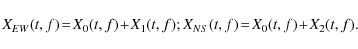
We now consider the correlation between signals from the two
antenna branches. Each beam can be assumed to be the sum of one pencil
beam with two confusion lobes (i.e., the parts of the main lobe
outside the pencil beam). We denote as E0(t) the electric field of
the wave received from the pencil beam, E1(t), the corresponding
field from the confusion lobes of the EW branch, and E2(t), the field from
the confusion lobes of the NS branch. After combining the outputs
from the two branches at the input of the ADC and performing
baseband digitization (e.g., at 66 MHz sampling frequency), we derive
two real-valued waveforms:
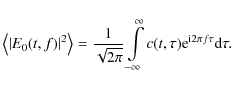
In estimating in real-time the spectral power of the waves approaching the pencil beam, i.e.,
- 1.
- to compute the cross-correlation of the two waveforms (data streams), i.e.,
the average convolution between the two signals
The averaging should be performed over a time interval that is much longer than the typical period(s) of the signal of interest (i.e., ). Substituting Eqs. (4) into (5) and using the
linearity of convolution and averaging operations, we have
). Substituting Eqs. (4) into (5) and using the
linearity of convolution and averaging operations, we have

= 
The last three terms are small (uncorrelated signals) and hence can be discarded, while the first one corresponds to the autocorrelation of the pencil beam electric field. Using the Wiener-Khinchin theorem, the Fourier transform (FT) of infers the power spectrum
in the pencil beam
infers the power spectrum
in the pencil beam
- 2.
- Alternately, we can first compute the spectra
XEW,NS(t,f) of each waveform in accordance with
Eq. (2). Owing to the linearity of FT, we obtain
Next, we can introduce the average of their cross product as
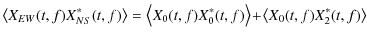
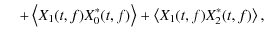
where the averaging is performed over elementary spectra.
The last three terms should vanish in the limit
elementary spectra.
The last three terms should vanish in the limit
 ,
and we again obtain
,
and we again obtain
Taking all the above considerations into account, the optimal way to obtain the ``pencil beam spectra'' in correlation mode (that has been accepted and implemented in the receiver) is as follows: (i) performing both the windowing and FFT of each waveform; followed by (ii) clipping of values above a given threshold; (iii) deriving the cross product of one NS spectrum by the complex conjugate of the corresponding EW one; and (iv) averaging over several products of complex spectra before calculating the squared amplitude of the average.
5 Applications
![\begin{figure}
\par\includegraphics[width=14cm,clip]{13335fg2.eps}
\end{figure}](/articles/aa/full_html/2010/02/aa13335-09/img55.png)
|
Figure 2: Spectrograms of Jupiter S-bursts calculated from a waveform recorded on March 13, 2005. a) Time and frequency resolutions are 2 ms and 4 kHz, respectively. The fine structure of the S-burst patterns is blurred; b) time and frequency resolutions are 0.25 ms and 4 kHz, respectively; c) zoomed image of the area enclosed by white rectangle in plate b). |
| Open with DEXTER | |
We discuss two examples of using the receiver to observe decameter radio sources that produce non-trivial patterns in the dynamic spectrograms.
5.1 Jovian S-bursts
![\begin{figure}
\par\includegraphics[width=16cm,clip]{13335fg3.eps}
\end{figure}](/articles/aa/full_html/2010/02/aa13335-09/img56.png)
|
Figure 3: Spectrograms of the pulsar PSR0809+74 recorded in full power mode. The grey-color scale represents the spectral power (white color corresponds to zero-intensity, the dark areas indicate powerful signals). a) Wide-band sequence of frequency-drifting pulses recorded on December 13, 2006; b) low-frequency pulses recorded on December 14, 2006 close to the ionospheric cut-off frequency, but still far above the limit imposed by the channel bandwidth (Eq. (8)) |
| Open with DEXTER | |
The S-burst emission occurs during so-called decameter radio storms, several-hour long events, which are predictable on the basis of the analysis of the geometric configuration between the Earth, Jupiter, and Io (Genova et al. 1989). Although the occurrence of S-bursts from Jupiter is predictable, the required temporal and frequency resolutions cannot be specified in advance because of the unpredictable morphology and rapid changes in S-burst shapes and fine structures. Therefore, an optimal solution for studying this type of emission is the waveform mode, when all the information within the receiver frequency-band is preserved, and the analysis of the time-frequency patterns is performed offline, after observation.
An example of using the waveform mode to observe Jupiter is shown
in Fig. 2, where we depict a fragment of an S-burst storm
recorded with the UTR-2 array on March 13, 2005. In Figs. 2a, b,
a spectrogram of duration ![]() 1 s calculated from the same
waveform but at different resolutions is shown. A characteristic
feature of the patterns seen in the spectrogram is the frequency
drift, i.e., a rapid change in the emission peak frequency with time.
The value of the frequency drift is of importance for testing
various models of the emission generation mechanism, magnetic field
of Jupiter, and plasma instabilities in the vicinity of Jupiter
(Hess et al. 2009; Zarka et al. 1996). The data presented in Fig. 2a was calculated at time and
frequency resolutions of 2 ms and 4 kHz, respectively. From the
visual inspection of this figure, one can conclude, for example, that
the two patterns numbered 1 and 2 are characterized by substantially
different values of the frequency drift. However, after increasing the
time resolution to 0.25 ms for a 4 kHz bandwidth, it becomes clear
that the pattern 2 (denoted as B in Figs. 2b, c) consists
of several frequency drifting components of approximately
similar frequency drift rate to the pattern 1 in Fig. 2a. A
zoomed version of the square area shown in Fig. 2b is
presented in Fig. 2c, which illustrates the complexity of the
intrinsic structure of the S-burst pattern.
1 s calculated from the same
waveform but at different resolutions is shown. A characteristic
feature of the patterns seen in the spectrogram is the frequency
drift, i.e., a rapid change in the emission peak frequency with time.
The value of the frequency drift is of importance for testing
various models of the emission generation mechanism, magnetic field
of Jupiter, and plasma instabilities in the vicinity of Jupiter
(Hess et al. 2009; Zarka et al. 1996). The data presented in Fig. 2a was calculated at time and
frequency resolutions of 2 ms and 4 kHz, respectively. From the
visual inspection of this figure, one can conclude, for example, that
the two patterns numbered 1 and 2 are characterized by substantially
different values of the frequency drift. However, after increasing the
time resolution to 0.25 ms for a 4 kHz bandwidth, it becomes clear
that the pattern 2 (denoted as B in Figs. 2b, c) consists
of several frequency drifting components of approximately
similar frequency drift rate to the pattern 1 in Fig. 2a. A
zoomed version of the square area shown in Fig. 2b is
presented in Fig. 2c, which illustrates the complexity of the
intrinsic structure of the S-burst pattern.
5.2 Low-frequency pulsar observations
In the second example, we consider the radio emission from pulsars
in the decameter waveband. Pulsars are rotating neutron stars that
are known as bright radio sources. The emission consists of periodic
pulses produced by a rotating object into a sharply beamed radiation
pattern. Every time the beam hits the Earth observer, a pulse of
emission can be detected, in a similar way to a lighthouse. The pulses of
emission are broad-band, i.e., the frequencies at which various
pulsars have been found range from the X- and ![]() -rays to the
decameter wave band. It should be noted, however, that because of the
absence until now of high-sensitivity, interference-immune receiver
systems, pulsar emission in the decameter waveband has remained
practically unexplored.
-rays to the
decameter wave band. It should be noted, however, that because of the
absence until now of high-sensitivity, interference-immune receiver
systems, pulsar emission in the decameter waveband has remained
practically unexplored.
Although at their origin the pulses are emitted at all frequencies simultaneously, they experience subsequent distortion in the time-frequency plane defined by the dispersion of radio waves propagating in the interstellar medium. In terms of dynamic spectrogram analysis, this means that initially vertical lines in the dynamic spectra corresponding to individual pulses are transformed at the reception point into frequency drifting stripes of emission with a frequency-dependent drift rate. A typical spectrogram of the powerful pulsar PSR0809+74 is shown in Fig. 3a. Dark lines crossing the spectrogram from high to low frequencies are intense single pulses dispersed by the interstellar medium. It should also be noted that the high sensitivity spectrogram shown in Fig. 3a allows us to distinguish between the effects of interplanetary scintillations (Gapper et al. 1982) (broad vertical intensity modulation bands) and pulse-to-pulse variations in power at the source (Ritchings 1976) (some of the dispersed pulses look brighter than their neighbours).
The law of interstellar dispersion is well-known (Manchester & Taylor 1977)
and described by the equation
![\begin{displaymath}\Delta t =
10^7\left(\frac{1}{f_1^2}-\frac{1}{f_2^2}\right)\frac{\rm DM}{2.41}~\left[\rm ms\right] ,
\end{displaymath}](/articles/aa/full_html/2010/02/aa13335-09/img58.png)
where
![\begin{displaymath}{\rm DM}=\int{n_{\rm e}~{\rm d}l}=\left\langle n_{\rm e}\right\rangle D~\left[\rm pc~
cm^{-3}\right] ,
\end{displaymath}](/articles/aa/full_html/2010/02/aa13335-09/img59.png)
where
![\begin{displaymath}\frac{{\rm d}f}{{\rm d}t}=kf^3~\left[\frac{\rm MHz}{\rm s}\right] ,
\end{displaymath}](/articles/aa/full_html/2010/02/aa13335-09/img61.png)
where
| Figure 4: Schematic of a periodic sequence of frequency-drifting pulses crossing a frequency channel of the spectrum analyzer. |
|
| Open with DEXTER | |
The time ![]() is an interval between successive pulses in the
output of an elementary frequency channel of the spectrogram. The
two pulses can be resolved if
is an interval between successive pulses in the
output of an elementary frequency channel of the spectrogram. The
two pulses can be resolved if ![]() ,
i.e., the pulses do not
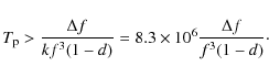
overlap. The condition of non-overlap can be formulated in terms of
the frequency bandwidth
,
i.e., the pulses do not
overlap. The condition of non-overlap can be formulated in terms of
the frequency bandwidth ![]() of a frequency channel, the
frequency drift rate defined by Eq. (7), the dispersion
measure DM, the pulsar period
of a frequency channel, the
frequency drift rate defined by Eq. (7), the dispersion
measure DM, the pulsar period ![]() ,
and the duty cycle of the
pulsar, d, which is the fraction of time when the emission intensity is
above the noise level. The duty cycle of pulsars varies and is
frequency dependent, but is typically in the range
,
and the duty cycle of the
pulsar, d, which is the fraction of time when the emission intensity is
above the noise level. The duty cycle of pulsars varies and is
frequency dependent, but is typically in the range
![]() (Kuzmin et al. 1998).
(Kuzmin et al. 1998).
From the sketch in Fig. 4, one can infer that
where
Here,
It should also be noted that due to scattering processes
in the interstellar medium, the pulse experiences additional frequency
dependent broadening (Bhat et al. 2004), i.e., an additional term
![]() should also be subtracted from the value of
should also be subtracted from the value of ![]() .
In the case of a
power-law spectrum of wave numbers in the scattering medium,
.
In the case of a
power-law spectrum of wave numbers in the scattering medium,
![]() follows the power law
follows the power law
![]() ,
where
,
where ![]() takes the value of 4.4 for a Kolmogorov-type spectrum.
In the subsequent analysis, we, however, neglect this additional
pulse broadening by assuming that its magnitude is much smaller than
that defined by the dispersion measure, i.e.,
takes the value of 4.4 for a Kolmogorov-type spectrum.
In the subsequent analysis, we, however, neglect this additional
pulse broadening by assuming that its magnitude is much smaller than
that defined by the dispersion measure, i.e.,
![]() .
.
For the parameter values used in our observations with the UTR-2 array,
i.e., a sampling frequency
![]() MHz, and a time window size of
MHz, and a time window size of
![]() defining the frequency channel separation at
defining the frequency channel separation at
![]() kHz), one can estimate which pulsars can be detected, e.g., by
visual inspection of the dynamic spectra in the full power mode. In
Fig. 5, we plot a scatter diagram of the values of DM versus
kHz), one can estimate which pulsars can be detected, e.g., by
visual inspection of the dynamic spectra in the full power mode. In
Fig. 5, we plot a scatter diagram of the values of DM versus
![]() for 56 pulsars (Kuzmin et al. 1998) and also for the
Crab pulsar. Four solid lines, obtained with Eq. (8) at
frequencies
f=6,10,10,10 MHz for a value of duty cycle
for 56 pulsars (Kuzmin et al. 1998) and also for the
Crab pulsar. Four solid lines, obtained with Eq. (8) at
frequencies
f=6,10,10,10 MHz for a value of duty cycle
![]() are also shown, together with dashed lines
calculated at the value of d=0.15 (corresponding to a
are also shown, together with dashed lines
calculated at the value of d=0.15 (corresponding to a ![]()
![]() pulse profile width). The small distance between the
solid and dashed lines indicates that the main part of the pulse
distortion is defined by the dispersion time
pulse profile width). The small distance between the
solid and dashed lines indicates that the main part of the pulse
distortion is defined by the dispersion time ![]() ,
so that a
non-zero value of the duty cycle d can be neglected for an
approximate analysis of almost all the pulsars considered here.
,
so that a
non-zero value of the duty cycle d can be neglected for an
approximate analysis of almost all the pulsars considered here.
![\begin{figure}
\par\includegraphics[width=7cm,clip]{13335fg5.eps}
\end{figure}](/articles/aa/full_html/2010/02/aa13335-09/img81.png)
|
Figure 5:
Dispersion measure vs. period for 56 pulsars
(Kuzmin et al. 1998) (diamonds) and for the Crab pulsar (crossed diamond).
Four lines calculated with Eq. (8), corresponding to the
frequencies of 6, 10, 20, and 30 MHz, delimit the lower limits of the areas
where the pulsars can be detected with a receiver of 4 kHz frequency
resolution. Solid and dashed lines correspond to different values of
the parameter d defining the pulsar duty cycle: d=0 and d=0.15,
respectively. For example, the pulsar PSR0809+74 (crossed diamond)
is observable at any frequency above |
| Open with DEXTER | |
All the points shown in Fig. 5, except the one of the Crab pulsar, are located below the line f=30 MHz and, therefore, these pulsars are resolved by the 4 kHz frequency channels. The pulses from the Crab pulsar cannot be detected in the decameter waveband with a 16 384-point FFT at sampling frequency 66 MHz. On the other hand, it is possible to resolve these pulses in the waveform mode if it is set to the frequency resolution at 0.25 kHz by using a 262 144-point FFT in the post-processing. In such case, the point corresponding to the Crab pulsar shifts to the region of detectability between the lines of 10 MHz and 20 MHz in Fig. 5, therefore the pulse sequences should become visible in the frequency range 10 MHz <f< 20 MHz.
We note that the alternative method of coherent dedispersion (Lorimer & Kramer 2005) can be applied to waveform data to compensate for the effect of the interstellar medium. This method is renowned for achieving greater timing accuracy in studying the pulse profiles and, moreover, it can easily be implemented into software. Once the data is recorded in the waveform mode, the advantage of building an optimal coherent dedispersion algorithm can be taken in subsequent processing.
Many pulsars that appear between the lines at f=10 MHz and f=30 MHz in Fig. 5 can thus be successfully observed within the
observational band of the UTR-2 array (8-32 MHz). It should be
noted, however, that because of decay of the radio waves in the
ionosphere at low frequencies, the detection of individual pulses
below ![]() 12 MHz is a rare event in observations with UTR-2, which
occurs only for the most powerful pulsars, e.g., PSR0809+74
shown in Fig. 3. Despite the low SNR and slow frequency
drift rate, two pulses can be clearly identified by eye in
Fig. 3b.
12 MHz is a rare event in observations with UTR-2, which
occurs only for the most powerful pulsars, e.g., PSR0809+74
shown in Fig. 3. Despite the low SNR and slow frequency
drift rate, two pulses can be clearly identified by eye in
Fig. 3b.
We finally sort in Table 2 the pulsars according to their observability with the full power mode at 4 kHz frequency resolution. The pulsars in the first column can be observed in a wide frequency band, sometimes even below 10 MHz. The second and third columns contain pulsars that are resolved in the upper frequency part of the spectrogram only. The pulsars in the last column may be problematic to observe at 4 kHz resolution. The individual pulses from those pulsars are expected to be resolved only when observed in the waveform mode.
Table 2: Pulsar list from (Kuzmin et al. 1998).
6 Conclusion
Using up-to-date digital components that have become commercially available, interference-immune design, and optimized real-time signal processing algorithms, we have developed a digital receiver that has strong potential to obtain high-resolution spectral images in LF radio astronomy.To our knowledge, receivers combining characteristics such as multiple working regimes, high sensitivity, low level of spurious signals, and software interfaces adapted for LF radio observations have not been reported to date. As illustrated by two examples of observations performed with the receiver in the decameter wave band, the receiver has a high flexibility of operation modes, i.e., the working parameters can be tuned to optimize the reception of both sporadic and stationary types of radio signals. Besides the exploration of the radio emission from well-known objects such as Jupiter, Sun, and pulsars, the receiver can also be used for detecting and analyzing other radio sources, previously unexplored with ground-based instruments. Those include, for example, Saturn's lightning (Griessmeier et al. 2008), flaring stars (Abranin et al. 1997; Konovalenko et al. 2008), the elusive radio emission from exoplanets (Ryabov et al. 2004b; Weber et al. 2007).
Non-trivial fine spectral structures, unresolved by previously existing receiver equipment, are detected in the high-resolution spectrograms of Jupiter S-burst emissions. We found that many of the complex S-burst spectral patterns in the time-frequency plane consist of elementary coherent sub-bursts of duration 5-10 ms. A typical example of this division of large spectral patterns into smaller ones is presented in Fig. 2c. This property of S-burst patterns is a new finding, and will be studied further in a separate paper.
Another important but poorly studied class of decameter radio sources, radio pulsars, has also been discussed in the paper. The requirement of a receiver system capable of resolving powerful sequences of individual pulses (possibly including giant pulses (Cordes et al. 2004)) in the spectrograms is formulated in terms of the pulsar period and duty cycle, taking also into account wave propagation effects. An example showing the feasibility of observing separate pulses from the pulsar PSR0809+74 is given, down to the low-frequency limit determined by the Earth's ionospheric cutoff. An estimate of the parameters necessary to detect sequences of pulses is also formulated for the Crab pulsar as well as many other pulsars previously studied at higher frequencies.
AcknowledgementsThe receiver had been created, installed and commissioned within the framework of joint France-Japan-Ukraine-Austria project CNRS/ANR projectNT05-1_42530 ``The direct detection (and study) of exoplanets using radio waves''.
Appendix A: Receiver performance and technical solutions
![\begin{figure}
\par\includegraphics[width=7cm,clip]{13335fA1.eps}
\end{figure}](/articles/aa/full_html/2010/02/aa13335-09/img84.png)
|
Figure A.1: Signal path from the antenna system to the control display of the host computer. a) UTR-2 antenna array; b) anti-alias filters and amplifiers block; c) ADC module; d) DSP board to be plugged into a PCI-X slot of the host PC; e) snapshot of the host PC display during an observation session. |
| Open with DEXTER | |
The receiver concept is based on direct baseband data recording without any frequency conversion. This approach allows us to avoid difficulties caused by strong in-band interference signals. The hardware of the digital receiver consists of two parts (see Figs. A.1c, d): an ADC module and a DSP board. A block diagram of the receiver is shown in Fig. A.2. The ADC and DSP boards are connected either via a two-channel 5Gbit/sec serial data link (if both boards are installed in a single host PC) or optical fibers providing data transfer over a long distance (up to 10 km). In the ADC module, LTC2208 16-bit A/D converters are used. Data buffers and channel logics are realized with the FPGA Spartan3. The input data streams can be sampled at any rate defined by either internal or external clock, up to 130 MHz.
The DSP board design is based on the Xilinx Virtex-II 3000 chip used as a FPGA (field-programmable gate array), and, in addition, has a fixed-point signal processor TMS320C6416 and a 256 Mbyte on-board SDRAM memory module. The DSP board is designed as a PCI-X extension card, which supports the PCI-X64/66 standard interface for the communication with the host PC. Different modes of signal processing can be achieved by the receiver using the FPGA and the signal processor capabilities.
To reduce the impact of spurious signals generated in the DSP board and other circuits of the host PC, the ADC module is manufactured as a separate block . This engineering solution, as well as the elaborate shielding of sensitive elements, allowed us to achieve both a high SFDR value and a low level of noise floor (see Table 1). In particular, the SFDR parameter is crucial for radio astronomical observations, where weak signals from natural radio sources should be detected with the background of powerful in-band interference of terrestrial origin (mostly man-made). Therefore, serious efforts were undertaken to increase the SFDR-value. Among them, we mention an automatic digital DC bias compensation, and data dithering performed while transferring data to the DSP board via the serial link. The theoretical maximum SNR (or dynamic range) for the 16-bit LTC2208 A/D converter used is 78 dBFS, whereas an effective value of 74 dBFS was practically achieved.
The digitized data flow from the ADC is supplied to the DSP board, where a real-time, windowed FFT with or without a 50%-overlap, as well as spectral averaging, are performed in the FPGA. A modified 16 384-point FFT algorithm was implemented in the receiver that provides access to 8192 frequency channels. To improve the performance of the FFT calculation, a method of computing a single complex FFT for two real-valued signals (from the two input channels) with subsequent data re-ordering was applied. The windowing is realized via multiplication by values of window-function coefficients of 18 bits precision, which is downloaded to the DSP memory as a table of values at the stage of initializing the receiver before the start of data recording.
The fixed-point, digital signal processor TMS320C6416 provides an additional computing power, and is used to control the data transfer from the FPGA to the PCI-X controller and perform extra calculations, if necessary. For example, it is possible, when the signal processor is used in combination with the on-board RAM memory buffer, to implement real-time algorithms of RFI mitigation in the frequency domain, and/or compensate for a non-uniformity of the frequency response function of the antenna system.
In the waveform mode, the receiver is capable of continuous data transfer at a maximum rate of 260 Mbyte/sec via the PCI-X64/66 interface for writing the data to the array of hard disks organized as a RAID-0 system in the host computer.
For controlling the receiver parameters, the data acquisition process, and the real-time display, original software was developed. The software operates under the Windows'NT/2K/XP operating system and is organized as a network server. The introduction of LAN support and control of the receiver ensures various possible modes of remote diagnostics and parameter adjustment. For example, a regime of remote operation is essential in long-duration unattended observations, when the interaction of the observer with the data acquisition process is not required within, say, a night of observations. An example of the receiver control panel and real-time data visualization display is given in Fig. A.3.
![\begin{figure}
\par\includegraphics[width=14.8cm,clip]{13335fA2.eps}
\end{figure}](/articles/aa/full_html/2010/02/aa13335-09/img85.png)
|
Figure A.2: Block diagram of the receiver and data flow. |
| Open with DEXTER | |
![\begin{figure}
\par\includegraphics[width=14.8cm,clip]{13335fA3.eps}
\end{figure}](/articles/aa/full_html/2010/02/aa13335-09/img86.png)
|
Figure A.3: Example of the host computer screen during a session of observing Jupiter. |
| Open with DEXTER | |
Other characteristics of the receiver should also be mentioned. The receiver has a perfect linearity over its full dynamic range, and a calibration mode. A specific software allows us to use the receiver in an unattended mode, i.e., for automated observations of several radio sources. It can also be used as a component of more complicated astronomical data acquisition systems in combination with filtering system designed for observing specific radio sources and augmented with real-time RFI mitigation techniques. Further options include a choice of windowing function in FFT, pre-selection of the frequency band to be recorded to the hard disk (programmable bands), automated script control of the observation sessions, digital down-conversion of the observation frequency band, and implementation of automatic gain control for compensating the frequency response of the antenna, cables, preamplifiers, and input filter system.
Appendix B: Using a receiver in correlation mode with the UTR-2 array
![\begin{figure}
\includegraphics[width=12cm,clip]{13335fB1.eps}
\end{figure}](/articles/aa/full_html/2010/02/aa13335-09/img87.png)
|
Figure B.1: Computer simulation of the effect of suppressing the confusion signal by using cross-correlated spectra. a) Power spectrum of the signal in the NS-array containing two harmonic components and background noise; b) same as a), but for the EW array, where the third harmonic component corresponds to the confusion signal; c) spectrum of the sum of the signals from the two arrays in the simple full power mode; d) coherence function, i.e., the averaged complex product of the two complex spectra, where the confusion component is fully suppressed. |
| Open with DEXTER | |
- EW-array: two harmonic components of dimensionless amplitudes A1=0.05, A2=0.075,
and frequencies f1=21.0, f2=24.2 coming from the common part of the beams (pencil beam)
plus a confusion harmonic component of amplitude A3=0.1 and frequency f3=25.2.
Two independent realizations
 of white Gaussian noise and unit variance were
added to both parts simulating the sky background fluctuations in the pencil beam and the remaining
part of the EW-lobe.
of white Gaussian noise and unit variance were
added to both parts simulating the sky background fluctuations in the pencil beam and the remaining
part of the EW-lobe.
- NS-array: the same two harmonic components and noise originating in the pencil beam and
another independent Gaussian noise component
 representing the sky background fluctuations.
| EEW(t) | = | E0(t)+E1(t), | |
| E0(t) | = | ||
| E1(t) | = | ||
| ENS(t) | = | E0(t)+E2(t), | |
| E2(t) | = |
where
Appendix C: Acronyms
ADC Analog to Digital Converter dBc deciBels relative to the carrier dBFS deciBels relative to Full Scale DM Dispersion Measure DSP Digital Signal Processor ENOB Effective Number Of Bits (F)FT (Fast) Fourier Transform FPGA Field-Programmable Gate Array ITU International Telecommunication Union HF High Frequencies (<30 MHz) LEO Low Earth Orbit LF Low Frequencies LOFAR LOw Frequency ARray LWA Long Wavelength Array RFI Radio Frequency Interference SFDR Spurious Free Dynamic Range SNR Signal to Noise Ratio UTR-2 Ukrainian T-shape Radiotelescope Mark 2 VHF Very High Frequencies (> 30 MHz)
References
- Abranin, E. P., Bazelyan, L. L., Alekseev, I. Y., et al. 1997, Ap&SS, 257, 131 [Google Scholar]
- Bendat, J. S., & Piersol, A. G. 1986, Random data. Analysis and Measurement Procedures (New York: Wiley) [Google Scholar]
- Bhat, N. D. R., Cordes, J. M., Camilo, F., et al. 2004, ApJ, 605, 759 [CrossRef] [Google Scholar]
- Boischot, A., Rosolen, C., Aubier, M. G., et al. 1980, Icarus, 43, 399 [NASA ADS] [CrossRef] [Google Scholar]
- Braude, S. Y., Megn, A. V., Ryabov, B. P., et al. 1978, Ap&SS, 54, 3 [NASA ADS] [CrossRef] [Google Scholar]
- Briand, C., Zasvlasky, A., Maksimovic, M., et al. 2008, A&A, 490, 3398 [NASA ADS] [CrossRef] [EDP Sciences] [Google Scholar]
- Cordes, J. M., Bhat, N. D. R., Hankins, T. H., et al. 2004, ApJ, 612, 375 [NASA ADS] [CrossRef] [Google Scholar]
- Fitzgerald, W. J., Smith, R. L., Walden, A. T., & Young, P. C. 2000, Nonlinear and nonstationary signal processing (Cambridge: Cambridge Univ. Press) [Google Scholar]
- Gapper, G. R., Hewish, A., Purvis, A., & Duffet-Smith, P. J. 1982, Nature, 296, 633 [NASA ADS] [CrossRef] [Google Scholar]
- Genova, F., Zarka, P., & Lecacheux, A. 1989, in Time-variable Phenomena in the Jovian System, ed. M. J. S. Belton, R. A. West, & J. Rahe (NASA SP-494), 156 [Google Scholar]
- Griessmeier, J.-M., Zarka, P., Konovalenko, A., et al. 2008, Geophys. Rese. Abstracts, 10, EGU2008-A-09350 [Google Scholar]
- Hess, S., Zarka, P., Mottez, F., & Ryabov, V. B. 2009, P&SS, 57, 23 [Google Scholar]
- Johnson, J. T., Niamsuwan, N., & Ellingson, S. W. 2005, in Proceedings of the 2005 Earth-Sun System Technology Conference (ESTC2005), June 28-30, Maryland, USA [Google Scholar]
- Kleewein, P. C., Rosolen, C., & Lecacheux, A. 1997, in Planetary Radio Emissions IV, ed. H. O. Rucker, S. J. Bauer, & A. Lecacheux (Vienna: Austrian Acad. Sci. Press), 349 [Google Scholar]
- Konovalenko, A. A., Rucker, H. O., Lecacheux, A., et al. 2008, Geophys. Res. Abstracts, 10, EGU2008-A-08201 [Google Scholar]
- Kuzmin, A. D., Izvekova, V. A., Shitov, Yu. P., et al. 1998, A&AS, 127, 355 [Google Scholar]
- Lecacheux, A., Konovalenko, À. À., & Rucker, Í. Î. 2004, P&SS, 52, 1357 [NASA ADS] [CrossRef] [Google Scholar]
- Lorimer, D. R., & Kramer, M. 2005, Handbook of Pulsar Astronomy (Cambridge: Cambridge University Press) [Google Scholar]
- Manchester, R. N., & Taylor, J. H. 1977, Pulsars (San Francisco: Freeman) [Google Scholar]
- Melnik, V. N., Rucker, H. O., Konovalenko, A. A., et al. 2008, in Sol. Phys. Res. Trends, ed. P. Wang (New York: Nova Sci. Publ.), 287 [Google Scholar]
- Ritchings, R. T. 1976, MNRAS, 176, 249 [NASA ADS] [Google Scholar]
- Rosolen, C., Clerc, V., & Lecacheux, À. 1999, Radio Sci. Bull. 291, 6 [NASA ADS] [Google Scholar]
- Ryabov, B. P., Zarka, P., Rucker, H. O., et al. 1997, in Planetary Radio Emissions IV, ed. H. O. Rucker, S. J. Bauer, & A. Lecacheux (Vienna: Austrian Acad. Sci. Press), 65 [Google Scholar]
- Ryabov, V. B., Zarka, P., & Ryabov, B. P. 2004a, in Proc. Of Joint AOGS 1st Annual Meeting & 2nd APHW Conference, 5-9 July, Singapore, 385 [Google Scholar]
- Ryabov, V. B., Zarka, P., & Ryabov, B. P. 2004b, P&SS, 52, 1479 [NASA ADS] [CrossRef] [Google Scholar]
- Ryabov, V. B., Ryabov, B. P., Vavriv, D. M., et al. 2007, JGR, 112, A09206 [Google Scholar]
- Smith, J. O. 2007, Mathematics of the Discrete Fourier Transform (DFT): with Audio Applications (W3K Publishing) [Google Scholar]
- Tukey, J. W. 1967, in. Spectral analysis of time series, ed. B. Harris (John Wiley and sons) [Google Scholar]
- Weber, R., & Faye, C. 1998, in Signal Analysis and Prediction, ed. Prochazka et al. (Boston: Birkhauser) [Google Scholar]
- Weber, R., Viou, Ñ., Coffre, À., et al. 2005, EURASIP Journal în Applied Signal Processing, 16, 2686 [Google Scholar]
- Weber, R., Zarka, P., Ryabov, V. B., et al. 2007, Proc. of EUSIPCO 2007 Conference, 3-7 September, Poznañ, Poland [Google Scholar]
- Zarka, P., Farges, T., Ryabov, B. P., et al. 1996, GRL, 23, 125 [CrossRef] [Google Scholar]
- Zarka, P., Queinnec, J., Ryabov, B. P., et al. 1997, in Planetary Radio Emissions IV, ed. H. O. Rucker, S. J. Bauer, & A. Lecacheux (Vienna: Austrian Acad. Sci. Press) [Google Scholar]
- Zarka, P., Treumann, R. A., Ryabov, B. P., & Ryabov, V. B. 2001, Ap&SS, 277, 293 [Google Scholar]
Footnotes
All Tables
Table 1: Characteristics of the digital receiver.
Table 2: Pulsar list from (Kuzmin et al. 1998).
All Figures
|
|
Figure 1: Sketch of the geometry of UTR-2 beams on the sky, when the source of interest is located in the common part of the EW and NS lobes. |
| Open with DEXTER | |
| In the text | |
|
|
Figure 2: Spectrograms of Jupiter S-bursts calculated from a waveform recorded on March 13, 2005. a) Time and frequency resolutions are 2 ms and 4 kHz, respectively. The fine structure of the S-burst patterns is blurred; b) time and frequency resolutions are 0.25 ms and 4 kHz, respectively; c) zoomed image of the area enclosed by white rectangle in plate b). |
| Open with DEXTER | |
| In the text | |
|
|
Figure 3: Spectrograms of the pulsar PSR0809+74 recorded in full power mode. The grey-color scale represents the spectral power (white color corresponds to zero-intensity, the dark areas indicate powerful signals). a) Wide-band sequence of frequency-drifting pulses recorded on December 13, 2006; b) low-frequency pulses recorded on December 14, 2006 close to the ionospheric cut-off frequency, but still far above the limit imposed by the channel bandwidth (Eq. (8)) |
| Open with DEXTER | |
| In the text | |
| |
Figure 4: Schematic of a periodic sequence of frequency-drifting pulses crossing a frequency channel of the spectrum analyzer. |
| Open with DEXTER | |
| In the text | |
|
|
Figure 5:
Dispersion measure vs. period for 56 pulsars
(Kuzmin et al. 1998) (diamonds) and for the Crab pulsar (crossed diamond).
Four lines calculated with Eq. (8), corresponding to the
frequencies of 6, 10, 20, and 30 MHz, delimit the lower limits of the areas
where the pulsars can be detected with a receiver of 4 kHz frequency
resolution. Solid and dashed lines correspond to different values of
the parameter d defining the pulsar duty cycle: d=0 and d=0.15,
respectively. For example, the pulsar PSR0809+74 (crossed diamond)
is observable at any frequency above |
| Open with DEXTER | |
| In the text | |
|
|
Figure A.1: Signal path from the antenna system to the control display of the host computer. a) UTR-2 antenna array; b) anti-alias filters and amplifiers block; c) ADC module; d) DSP board to be plugged into a PCI-X slot of the host PC; e) snapshot of the host PC display during an observation session. |
| Open with DEXTER | |
| In the text | |
|
|
Figure A.2: Block diagram of the receiver and data flow. |
| Open with DEXTER | |
| In the text | |
|
|
Figure A.3: Example of the host computer screen during a session of observing Jupiter. |
| Open with DEXTER | |
| In the text | |
|
|
Figure B.1: Computer simulation of the effect of suppressing the confusion signal by using cross-correlated spectra. a) Power spectrum of the signal in the NS-array containing two harmonic components and background noise; b) same as a), but for the EW array, where the third harmonic component corresponds to the confusion signal; c) spectrum of the sum of the signals from the two arrays in the simple full power mode; d) coherence function, i.e., the averaged complex product of the two complex spectra, where the confusion component is fully suppressed. |
| Open with DEXTER | |
| In the text | |
Copyright ESO 2010
Current usage metrics show cumulative count of Article Views (full-text article views including HTML views, PDF and ePub downloads, according to the available data) and Abstracts Views on Vision4Press platform.
Data correspond to usage on the plateform after 2015. The current usage metrics is available 48-96 hours after online publication and is updated daily on week days.
Initial download of the metrics may take a while.