| Issue |
A&A
Volume 510, February 2010
|
|
|---|---|---|
| Article Number | A18 | |
| Number of page(s) | 17 | |
| Section | Interstellar and circumstellar matter | |
| DOI | https://doi.org/10.1051/0004-6361/200913076 | |
| Published online | 29 January 2010 | |
Radiation thermo-chemical models of protoplanetary disks
II. Line diagnostics
I. Kamp1 - I. Tilling2 - P. Woitke2 - W.-F. Thi3 - M. Hogerheijde4
1 - Kapteyn Astronomical Institute, Postbus 800,
9700 AV Groningen, The Netherlands
2 - UK Astronomy Technology Centre, Royal Observatory, Edinburgh,
Blackford Hill, Edinburgh EH9 3HJ, UK
3 - SUPA, Institute for Astronomy, Royal Observatory, Edinburgh,
Blackford Hill, Edinburgh EH9 3HJ, UK
4 - Leiden Observatory, Leiden University, PO Box 9513, 2300 RA Leiden, The Netherlands
Received 6 August 2009 / Accepted 4 November 2009
Abstract
Aims. In this paper, we explore the diagnostic power of the far-IR fine-structure lines of [O I] 63.2 ![]() m, 145.5
m, 145.5 ![]() m, [C II] 157.7
m, [C II] 157.7 ![]() m, as well as the radio and sub-mm lines of CO J=1-0,
2-1 and 3-2 in application to disks around Herbig Ae stars. We aim at
understanding where the lines originate from, how the line formation
process is affected by density, temperature and chemical abundance in
the disk, and to what extent non-LTE effects are important. The
ultimate aim is to provide a robust way to determine the gas mass of
protoplanetary disks from line observations.
m, as well as the radio and sub-mm lines of CO J=1-0,
2-1 and 3-2 in application to disks around Herbig Ae stars. We aim at
understanding where the lines originate from, how the line formation
process is affected by density, temperature and chemical abundance in
the disk, and to what extent non-LTE effects are important. The
ultimate aim is to provide a robust way to determine the gas mass of
protoplanetary disks from line observations.
Methods. We use the recently developed disk code P ROD IM O
to calculate the physico-chemical structure of protoplanetary disks and
apply the Monte-Carlo line radiative transfer code R ATRAN to predict observable line profiles and fluxes. We consider a series of Herbig Ae type disk models ranging from 10-6 ![]() to
to
![]()
![]() (between 0.5 and 700 AU) to discuss the dependency of the line
fluxes and ratios on disk mass for otherwise fixed disk parameters.
This paper prepares for a more thorough multi-parameter analysis
related to the Herschel open time key program G ASPS.
(between 0.5 and 700 AU) to discuss the dependency of the line
fluxes and ratios on disk mass for otherwise fixed disk parameters.
This paper prepares for a more thorough multi-parameter analysis
related to the Herschel open time key program G ASPS.
Results. We find the [C II] 157.7 ![]() m line to originate in LTE from the surface layers of the disk, where
m line to originate in LTE from the surface layers of the disk, where
![]() .
The total emission is dominated by surface area and hence depends strongly on disk outer radius. The [O I] lines can be very bright (>10-16 W/m2) and form in slightly deeper and closer regions under non-LTE conditions. For low-mass models, the [O I]
lines come preferentially from the central regions of the disk, and the
peak separation widens. The high-excitation [O I] 145.5
.
The total emission is dominated by surface area and hence depends strongly on disk outer radius. The [O I] lines can be very bright (>10-16 W/m2) and form in slightly deeper and closer regions under non-LTE conditions. For low-mass models, the [O I]
lines come preferentially from the central regions of the disk, and the
peak separation widens. The high-excitation [O I] 145.5 ![]() m line, which has a larger critical density, decreases more rapidly with disk mass than the 63.2
m line, which has a larger critical density, decreases more rapidly with disk mass than the 63.2 ![]() m line. Therefore, the [O I] 63.2
m line. Therefore, the [O I] 63.2 ![]() m/145.5
m/145.5 ![]() m ratio is a promising disk mass indicator, especially as it is independent of disk outer radius for
m ratio is a promising disk mass indicator, especially as it is independent of disk outer radius for
![]() AU. CO is abundant only in deeper layers
AU. CO is abundant only in deeper layers
![]() .
For too low disk masses (
.
For too low disk masses (
![]() )
the dust starts to become transparent, and CO is almost completely
photo-dissociated. For masses larger than that the lines are an
excellent independent tracer of disk outer radius and can break the
outer radius degeneracy in the [O I] 63.2
)
the dust starts to become transparent, and CO is almost completely
photo-dissociated. For masses larger than that the lines are an
excellent independent tracer of disk outer radius and can break the
outer radius degeneracy in the [O I] 63.2 ![]() m/[C II]157.7
m/[C II]157.7 ![]() m line ratio.
m line ratio.
Conclusions. The far-IR fine-structure lines of [C II] and [O I]
observable with Herschel provide a promising tool to measure the disk
gas mass, although they are mainly generated in the atomic surface
layers. In spatially unresolved observations, none of these lines carry
much information about the inner, possibly hot regions <30 AU.
Key words: astrochemistry - methods: numerical - line: formation - circumstellar matter - stars: formation - radiative transfer
1 Introduction
Observations of gas in protoplanetary disks are intrinsically difficult to interpret as they reflect the interplay between a complex chemical and thermal disk structure, statistical equilibrium and optical depth effects. This is particularly true if non-thermal excitation such as fluorescence or photodissociation dominate the statistical equilibrium.
The first studies of gas in protoplanetary disks concentrated
on the rotational transitions of abundant molecules such as CO, HCN and
HCO+ (e.g. Thi et al. 2004; Beckwith et al. 1986; Dutrey et al. 1997; van Zadelhoff et al. 2001; Koerner et al. 1993). Those lines originate in the outer regions of disks, r>100 AU, where densities are at most
![]() cm-3. The interpretation of those lines was mainly based on tools and expertise developed for molecular clouds. Using the CO J=3-2 line, Dent et al. (2005)
inferred for a sample of Herbig Ae and Vega-type stars a trend of disk
outer radius with age; on average, the outer disk radius in the
7-20 Myr range is three times smaller than that in the
<7 Myr range. Also, the disk radii inferred from the dust
spectral energy distribution (SED) are generally smaller than those
derived from the gas line (Piétu et al. 2005; Isella et al. 2007). Hughes et al. (2008a) suggest a soft outer edge as a solution to the discrepancy. Comparison of CO J=3-2 maps of four disks to different types of disk models strongly supports a soft edge in favor of a sharp cutoff. Piétu et al. (2007) use the CO and HCO+
lines to probe the radial and vertical temperature profile of the disk.
Simple power law disk models and LTE radiative transfer provides best
matching results for radial temperature gradients around r-0.5. The 12CO J=2-1 line, 13CO J=2-1 and 13CO J=1-0
lines used in their analysis probe subsequently deeper layers and
reveal a vertical temperature gradient ranging from 50 K in the
higher layers to below the freeze-out temperature of CO in the
midplane. This confirms earlier findings by Dartois et al. (2003).
cm-3. The interpretation of those lines was mainly based on tools and expertise developed for molecular clouds. Using the CO J=3-2 line, Dent et al. (2005)
inferred for a sample of Herbig Ae and Vega-type stars a trend of disk
outer radius with age; on average, the outer disk radius in the
7-20 Myr range is three times smaller than that in the
<7 Myr range. Also, the disk radii inferred from the dust
spectral energy distribution (SED) are generally smaller than those
derived from the gas line (Piétu et al. 2005; Isella et al. 2007). Hughes et al. (2008a) suggest a soft outer edge as a solution to the discrepancy. Comparison of CO J=3-2 maps of four disks to different types of disk models strongly supports a soft edge in favor of a sharp cutoff. Piétu et al. (2007) use the CO and HCO+
lines to probe the radial and vertical temperature profile of the disk.
Simple power law disk models and LTE radiative transfer provides best
matching results for radial temperature gradients around r-0.5. The 12CO J=2-1 line, 13CO J=2-1 and 13CO J=1-0
lines used in their analysis probe subsequently deeper layers and
reveal a vertical temperature gradient ranging from 50 K in the
higher layers to below the freeze-out temperature of CO in the
midplane. This confirms earlier findings by Dartois et al. (2003).
However, disk masses derived from the CO lines are in general lower than disk masses derived from dust observations (e.g. Thi et al. 2001; Zuckerman et al. 1995). Possible explanations include CO ice formation in the cold midplane and photodissociation in the upper tenuous disk layers. Any single gas tracer alone can only provide gas masses of the species and volume from which it originates, the same way as dust masses derived from a single photometric measurement are only sensitive to grains of a particular size range, namely those grain sizes that dominate the emission at that photometric wavelength. Hence individual gas tracers are more valuable for probing the physical conditions of the volume where they arise than the total disk mass. A combination of suitable gas tracers can then allow us to characterize the gas properties in protoplanetary disks and study it during the planet formation process.
This paper aims at exploring the diagnostic power of the fine structure lines of [O I] and [C II]
in the framework of upcoming Herschel observations. Earlier modeling of
these lines indicated that they should be detectable down to disk
masses of
![]() of gas, so also in the very gas-poor debris disks (Kamp et al. 2005). More recent work by Meijerink et al. (2008)
presents fine structure lines from the inner 40 AU disk of an
X-ray irradiated T Tauri disk; the models indicate that the [O I]
emission originates over a wide range of radii and depth and is
sensitive to the X-ray luminosity. However, most of the C II and O I line emission comes from larger radii where the gas temperature is dominated by UV heating processes. Jonkheid et al. (2007) find from thermo-chemical models of UV dominated Herbig Ae disks that the [O I] lines are generally a factor 10 stronger that the [C II] line. We started to explore the origin of the fine structure lines in Woitke et al. (2009a) and find that the [C II] 157.7
of gas, so also in the very gas-poor debris disks (Kamp et al. 2005). More recent work by Meijerink et al. (2008)
presents fine structure lines from the inner 40 AU disk of an
X-ray irradiated T Tauri disk; the models indicate that the [O I]
emission originates over a wide range of radii and depth and is
sensitive to the X-ray luminosity. However, most of the C II and O I line emission comes from larger radii where the gas temperature is dominated by UV heating processes. Jonkheid et al. (2007) find from thermo-chemical models of UV dominated Herbig Ae disks that the [O I] lines are generally a factor 10 stronger that the [C II] line. We started to explore the origin of the fine structure lines in Woitke et al. (2009a) and find that the [C II] 157.7 ![]() m line probes
the upper flared surface layers of the outer disk while the [O I] 63.2
m line probes
the upper flared surface layers of the outer disk while the [O I] 63.2 ![]() m line originates from the thermally decoupled surface layers inward of about 100 AU, above
m line originates from the thermally decoupled surface layers inward of about 100 AU, above
![]() .
The latter line is very sensitive to the gas temperature and might be used to distinguish between hot (
.
The latter line is very sensitive to the gas temperature and might be used to distinguish between hot (
![]() K) and cold (
K) and cold (
![]() )
disk atmospheres. Since the fine structure lines generally originate
from a wider radial and vertical range than for example the 12CO rotational lines, they are potentially more suitable gas mass tracers.
)
disk atmospheres. Since the fine structure lines generally originate
from a wider radial and vertical range than for example the 12CO rotational lines, they are potentially more suitable gas mass tracers.
We use in this paper the disk modeling code P ROD IM O presented in Woitke et al. (2009a) to study the gas line emission from disks around Herbig Ae stars. The main focus are the fine-structure lines of C II and O I which will be observed for a large sample of disks during the H ERSCHEL open time Key Program G ASPS (Gas evolution in protoplanetary systems: http://www.laeff.inta.es/projects/herschel). The disk parameters were chosen to resemble the disk around MWC480. According to previous work by Mannings et al. (1997), Thi et al. (2001) and Piétu et al. (2007), the disk around this star extends from ![]() 0.5 AU to 700 AU. We choose here a surface density profile
0.5 AU to 700 AU. We choose here a surface density profile
![]() r-1.0. The central star is an A2e Herbig star with a mass of 2.2
r-1.0. The central star is an A2e Herbig star with a mass of 2.2 ![]() and an effective temperature of 8500 K.
and an effective temperature of 8500 K.
Section 2 gives a short summary of the disk modeling approach. The line radiative transfer method, re-gridding and the atomic input data are described in Sect. 3. We then briefly discuss some basic properties of the Herbig Ae disk models (Sect. 4) before we present the fine-structure lines (Sect. 5) and conclude with a discussion of the diagnostic strength of fine structure line ratios and a comparison to previous ISO and submm observations (Sect. 6).
2 ProDiMo
ProDiMo is a recently developed code for computing the hydrostatic structure of protoplanetary disks. This code combines frequency-dependent 2D dust continuum radiative transfer, kinetic gas-phase and UV photo-chemistry, ice formation, and detailed non-LTE heating & cooling with the consistent calculation of the hydrostatic disk structure. Details can be found in Woitke et al. (2009a). We summarize in the following some other aspects that are particularly relevant to this study.
We use a P HOENIX stellar model Brott & Hauschildt (2005)
with an effective temperature of 8500 K for the stellar
irradiation and a highly diluted 20 000 K black body for the
IS radiation field that penetrates the disk from all sides. The dust
opacities are computed using Mie theory and optical constants from Draine & Lee (1984).
The chemical network contains 71 species (build from
9 elements) connected through 950 reactions (photo reactions, CR
ionization, neutral-neutral, ion-molecule, as well as grain adsorption
and desorption processes for CO, CO2, H2O, CH4 and NH3
ice). The gas temperature follows from an extensive heating and cooling
balance that includes fine-structure line cooling as well as molecular
and optical lines (fluorescence in the inner disk). The code does not
yet include X-ray heating. This seems a minor issue for Herbig stars
that generally have quite moderate X-ray luminosities,
![]() erg s-1 (e.g. Stelzer et al. 2006).
erg s-1 (e.g. Stelzer et al. 2006).
The treatment of photoionization and photodissociation in this work differs from that in the original code.
The photoionization and photodissociation rates,
![]() ,
are now computed at each grid point using the spectral photon energy density
,
are now computed at each grid point using the spectral photon energy density
![]() calculated by the 2D continuum radiative transfer and the cross-sections
calculated by the 2D continuum radiative transfer and the cross-sections
![]() from the Leiden database (van Dishoeck et al. 2008). The photorate for continuous absorption is
from the Leiden database (van Dishoeck et al. 2008). The photorate for continuous absorption is
|
(1) |
When the photoprocess is initiated by line absorption, the rate becomes
|
(2) |
where fj is the oscillator strength for absorption from lower level i to upper level j,
We compute a series of Herbig Ae disk models with masses between
![]() and
and
![]() .
The parameters are summarized in Table 1. The dust used in this model is typically larger than ISM dust and generates the
.
The parameters are summarized in Table 1. The dust used in this model is typically larger than ISM dust and generates the ![]()
![]() opacity law as derived from dust observations (e.g. Rodmann et al. 2006; Beckwith & Sargent 1991; Mannings & Emerson 1994).
opacity law as derived from dust observations (e.g. Rodmann et al. 2006; Beckwith & Sargent 1991; Mannings & Emerson 1994).
Table 1: Parameters of the Herbig Ae model series.
3 Line radiative transfer
3.1 Methods
We use the two-dimensional Monte Carlo radiative transfer code R ATRAN developed by Hogerheijde & van der Tak (2000). The code uses a two-step approach to solve the non-LTE line radiative transfer, A MC, and S KY. The first code solves the level population numbers for a given model atom/molecule within an arbitrary two-dimensional density and temperature distribution. The second one performs the ray tracing to derive the emission for a given line, distance and disk inclination. In the following, we discuss some aspects that are particularly relevant in applying these codes to complex chemical disk stratifications.
3.2 Re-gridding
The 2D non-LTE line transfer code R ATRAN requires a grid of
rectangular cells in cylindrical coordinates
![]() and
and
![]() which is different from the grid of points used
in P ROD IM O. Therefore, we have to create a suitable grid of
cells for R ATRAN and ``fill'' the cells in a physically sensible way, which will involve some kind of averaging for the physical quantities.
which is different from the grid of points used
in P ROD IM O. Therefore, we have to create a suitable grid of
cells for R ATRAN and ``fill'' the cells in a physically sensible way, which will involve some kind of averaging for the physical quantities.
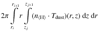
We choose to evaluate these mean values by integration and define the
following general function between the P ROD IM O grid points
|
(3) |
which can be applied to any physical quantity, e. g.species particle density
Next, we calculate the following integrals over the R ATRAN cells
| Vij | = | (4) | |
| = | 
|
(5) | |
| = | 
|
(6) | |
| = | 
|
(7) |
to derive mean values for the species density, gas and dust temperature in our R ATRAN cells
| |
= | (8) | |
| = | (9) | ||
| = | (10) |
Similar formulae apply to the collision partner densities. We have choosen this procedure (i) to assure total and species mass conservation; (ii) to conserve the total line emission in optically thin LTE at long wavelengths (Rayleigh-Jeans approximation); and (iii) to guaranty that the total thermal dust emission in the optically thin case (Rayleigh-Jeans approximation) is conserved.
Figure 1 shows how the R ATRAN grid compares to the original grid and underlying O I density distribution (10-2 ![]() model).
model).
![\begin{figure}
\par\includegraphics[width=9cm,height=6cm]{13076fg1.ps}
\vspace*{4mm}
\end{figure}](/articles/aa/full_html/2010/02/aa13076-09/img93.png)
|
Figure 1:
Distribution of cells for the R ATRAN radiative transfer code. The background contours show the O I density distribution of the
|
| Open with DEXTER | |
3.3 Modified radiative transfer code R ATRAN
The original R ATRAN code uses an accelerated Lambda iteration scheme to accelerate the convergence (Hogerheijde & van der Tak 2000). For rather complex molecules with a large number of levels heavily interconnected through lines of various strengths, such as water, the performance is too slow to allow a full exploration of the disk parameter space. We describe in the following the implementation of two additional methods that significantly improve the R ATRAN performance.
The line transfer simulations in R ATRAN are carried out in two stages, called the ``fixset'' and the ``random'' stages. During the fixset stage the number, starting points and directions of the rays are fixed, and only the non-local feedback between level populations and spectral intensities are solved iteratively. In order to accelerate the convergence during the random-noise-free fixset stage, we have included the procedure of Auer (1984) for strictly convergent transformations, known as the Ng-iteration. During the random phase, the number of rays is successively increased in all cells until three different sets of rays give approximately the same results.
The typical errors of the Monte-Carlo method depend on the
chosen set of random numbers. For standard (pseudo-random) number
generators, the errors decrease with the number of photon packages as N-1/2 (Niederreiter 1992).
Quasi-random numbers or low discrepancy sequences, to which the Sobol
sequence belongs, try to sample more uniformly the distributed points
(Sobol & Shukhman 2007; Press et al. 2002). The asymptotic errors of this quasi Monte-Carlo simulations
decrease as
![]() ,
where d is the dimension of the problem. For R ATRAN, the dimension is d=5,
because the position in the cell, the direction and the Doppler
velocity shift of the photon package are chosen randomly. The use of
quasi-random sequences
was already advocated by Juvela (1997),
since the gain in number of
photon packages is significant, but has not been widely adopted. One of
the main critics of quasi-random number sequences is that there are
only a limited number of sequences (Sloan 1993). Hybrid
methods called randomized or scrambled quasi-random sequences combine
the advantages of both individual methods, infinite number of
sequences and low error, resulting in an asymptotic noise that
decreases in
,
where d is the dimension of the problem. For R ATRAN, the dimension is d=5,
because the position in the cell, the direction and the Doppler
velocity shift of the photon package are chosen randomly. The use of
quasi-random sequences
was already advocated by Juvela (1997),
since the gain in number of
photon packages is significant, but has not been widely adopted. One of
the main critics of quasi-random number sequences is that there are
only a limited number of sequences (Sloan 1993). Hybrid
methods called randomized or scrambled quasi-random sequences combine
the advantages of both individual methods, infinite number of
sequences and low error, resulting in an asymptotic noise that
decreases in
![]() ,
where s is between 1 and
1.5 (Hickernell & Yue 2000). Scramble quasi-random sequences show the
fastest noise decrease among the three types of sequences.
,
where s is between 1 and
1.5 (Hickernell & Yue 2000). Scramble quasi-random sequences show the
fastest noise decrease among the three types of sequences.
We replaced the pseudo-random sequence in R ATRAN by the quasi-random Sobol
sequence combined with a Owen-Faure-Tezuka type of scrambling
(Owen 2003). A detailed description of the ACM
algorithm 659 implemented in R ATRAN is given by Bratley et al. (1994).
Difficult problems, like those involving water lines, require up to
108 photon packages with the standard random sequence but only
between 104 (s=1.5) and ![]()
![]() (s=1) photon
packages with the scrambled quasi-random sequence, a gain in CPU time
between 50 (s=1) and 104 (s=1.5). This speed gain opens the
possibility to study water line emissions from protoplanetary disks
with reasonable computing times (Woitke et al. 2009b).
(s=1) photon
packages with the scrambled quasi-random sequence, a gain in CPU time
between 50 (s=1) and 104 (s=1.5). This speed gain opens the
possibility to study water line emissions from protoplanetary disks
with reasonable computing times (Woitke et al. 2009b).
We extended the original code also to include a larger number of collision partners. This proofs to be important as in the original code, the density of the first collision partner is used to compute the dust continuum emission. However, the density of one of the collision partners does not always equal the total hydrogen number density, thus causing inconsistencies either in the dust emission or the collision rates. Moreover, some lines originate over a wide range of physical and chemical conditions, so that the dominant collision partner changes between the various disk regions (e.g. from atomic hydrogen and electrons in the low density regions to molecular hydrogen and electrons deeper into the disk).
3.4 Ray tracing
We assume for our generic disk a distance of 131 pc and and
inclination of 45 degrees. The pixel size (spatial resolution) is
0.05'' and the entire box has a size of
![]() to ensure that no emission is lost (disk diameter is 10''). The velocity resolution is set to 0.05 km s-1 and the total range is from -25 to 25 km s-1 for the C II line and -40 to 40 km s-1 for the O I
lines. The different velocity ranges reflect the differences in radial
origin of the lines. For the oxygen fine structure lines, oversampling
of the central pixels (out to 1.6'') was used, i.e. an additional 2
rays generated per pixel.
to ensure that no emission is lost (disk diameter is 10''). The velocity resolution is set to 0.05 km s-1 and the total range is from -25 to 25 km s-1 for the C II line and -40 to 40 km s-1 for the O I
lines. The different velocity ranges reflect the differences in radial
origin of the lines. For the oxygen fine structure lines, oversampling
of the central pixels (out to 1.6'') was used, i.e. an additional 2
rays generated per pixel.
The CO lines were computed within the same box of
![]() ,
but with a spatial resolution of 0.12'' and a spectral
resolution of 0.2 km s-1. No oversampling was used in this case.
,
but with a spatial resolution of 0.12'' and a spectral
resolution of 0.2 km s-1. No oversampling was used in this case.
3.5 Atomic and molecular data
Energy levels, statistical weights, Einstein A coefficients and collision cross sections are taken from the Leiden L AMBDA database (Schöier et al. 2005). Table 2 provides an overview of the C II, O I and CO data used in this work.
Table 2: Atomic and molecular data taken from the L AMBDA database (Schöier et al. 2005).
Table 3: Atomic and molecular data for the oxygen and carbon fine structure lines and the CO rotational lines.
3.6 Dust opacities
The dust opacities used in the radiative transfer code are consistent with the opacities used in the
computation of the disk model with P ROD IM O.
The choice of opacities impacts the continuum around the line, i.e. the
dust thermal emission. For oxygen, the low fine structure levels can be
pumped by the thermal dust background. We see differences of up to 50%
in the continuum fluxes around the O I fine
structure lines and up to 20% differences in the line emission itself
when we choose either the grain size distribution from Table 1 using optical constants from Draine & Lee (1984) or opacity tables from Ossenkopf & Henning (1994). The latter are based on an MRN size distribution for interstellar medium grains
![]() with sizes 5 nm < a < 0.25
with sizes 5 nm < a < 0.25 ![]() m. In this paper, the possibility of icy grain mantles or non-spherical shapes is not explored.
m. In this paper, the possibility of icy grain mantles or non-spherical shapes is not explored.
4 The disk models
We compute a series of six disk models with different disk masses (
![]() ,
10-2, 10-3, 10-4, 10-5 and 10-6
,
10-2, 10-3, 10-4, 10-5 and 10-6 ![]() )
and all other parameters remaining fixed. It is important to stress
that this series of models is not intended to reflect an evolutionary
sequence as we do not change the dust properties accordingly (e.g. dust
grain sizes, dust-to-gas mass ratio, settling). The goal is to explore
a range of physical conditions, study their impact on the disk
chemistry and analyze how this impacts the cooling radiation that will
be probed e.g. with the Herschel satellite.
)
and all other parameters remaining fixed. It is important to stress
that this series of models is not intended to reflect an evolutionary
sequence as we do not change the dust properties accordingly (e.g. dust
grain sizes, dust-to-gas mass ratio, settling). The goal is to explore
a range of physical conditions, study their impact on the disk
chemistry and analyze how this impacts the cooling radiation that will
be probed e.g. with the Herschel satellite.
![\begin{figure}
\par\includegraphics[width=18cm,clip]{13076fg2.eps}
\end{figure}](/articles/aa/full_html/2010/02/aa13076-09/img110.png)
|
Figure 2:
From top to bottom row: disk models with 10-2, 10-3, 10-4 and 10-5 |
| Open with DEXTER | |
![\begin{figure}
\par\includegraphics[width=17cm,clip]{13076fg3.eps}
\end{figure}](/articles/aa/full_html/2010/02/aa13076-09/img113.png)
|
Figure 3:
From top to bottom row: disk models with 10-2, 10-3, 10-4 and 10-5 |
| Open with DEXTER | |
4.1 Physical structure
Figure 2
provides an overview of the computed physical quantities such as gas
density, UV radiation field strength, optical extinction, gas
temperature and dust temperature resulting from our series of Herbig
disk models; each row presents a model with different mass and shows
three quantities, total hydrogen number density, UV radiation field
strength, and gas temperature. The white dashed lines in the second
column of this figure indicate the AV=1 and AV=10 surfaces. The
![]() model is optically thick in the vertical direction out to
model is optically thick in the vertical direction out to ![]() 400 AU. Reducing the disk mass by a factor 200 leaves only a dense
400 AU. Reducing the disk mass by a factor 200 leaves only a dense ![]() 10 AU wide optically thick ring and the low mass disk models (
10 AU wide optically thick ring and the low mass disk models (![]()
![]() )
have very low vertical extinction,
)
have very low vertical extinction,
![]() ,
throughout the entire disk.
,
throughout the entire disk.
The high mass models show two vertically puffed up regions, one around
0.5 AU (the classical ``inner rim''), the other one more radially
extended between 5 and 10 AU. The very low mass models (
![]() and
below) do not show the typical flaring disk structure as observed in
optically thick disk models, but they are still very extended in the
vertical direction. The extreme gas temperatures in these low mass
models are a result of direct heating by the photoelectric effect on
small dust grains (PAHs) and pumping of Fe II by the stellar radiation field. In these optically thin disks, coupling between gas and dust grains is not efficient.
and
below) do not show the typical flaring disk structure as observed in
optically thick disk models, but they are still very extended in the
vertical direction. The extreme gas temperatures in these low mass
models are a result of direct heating by the photoelectric effect on
small dust grains (PAHs) and pumping of Fe II by the stellar radiation field. In these optically thin disks, coupling between gas and dust grains is not efficient.
4.2 Chemical structure
The particle densities of ionized carbon, oxygen and the abundance of CO are shown in Fig. 3. The oxygen abundance is rather constant throughout the disks (C/O ratio ![]() 0.45),
being only lower by a factor of two where the CO and OH abundances are
high; OH forms at high abundance inside 30 AU above an AV
of a few, thus co-spatial with the warm (>200 K) CO gas.
Extremely low abundances occur only if significant amounts of water
form close to the midplane inside 1-10 AU (
0.45),
being only lower by a factor of two where the CO and OH abundances are
high; OH forms at high abundance inside 30 AU above an AV
of a few, thus co-spatial with the warm (>200 K) CO gas.
Extremely low abundances occur only if significant amounts of water
form close to the midplane inside 1-10 AU (
![]() -
-
![]() models).
models).
Carbon is fully ionized in the disk models with masses below
![]() .
The C+ abundance is complementary to the CO abundance as the neutral carbon layer between them is very thin. The C+/C/CO transition is governed by PDR physics and can be well defined using the classical PDR parameter
.
The C+ abundance is complementary to the CO abundance as the neutral carbon layer between them is very thin. The C+/C/CO transition is governed by PDR physics and can be well defined using the classical PDR parameter
![]() .
Above
.
Above
![]() (see Fig. 3),
carbon is fully ionized and its density structure resembles that of the
total gas density (two puffed up inner rims). The column density of the
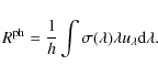
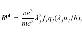
ionized carbon layer is always smaller than a few times 1017 cm-3. The mass of C+
in the irradiated layers of the disk is roughly constant until the
optically thin disk limit is reached in which case it is given by
(see Fig. 3),
carbon is fully ionized and its density structure resembles that of the
total gas density (two puffed up inner rims). The column density of the
ionized carbon layer is always smaller than a few times 1017 cm-3. The mass of C+
in the irradiated layers of the disk is roughly constant until the
optically thin disk limit is reached in which case it is given by
![]() (see Table 4).
(see Table 4).
High abundances of CO can be found down to disk masses of
![]() .
Below that, the entire disk becomes optically thin (radially and
vertically), thus reducing the CO abundances even in the midplane to
values below 10-6. In the models with masses above
.
Below that, the entire disk becomes optically thin (radially and
vertically), thus reducing the CO abundances even in the midplane to
values below 10-6. In the models with masses above
![]() ,
densities in the innermost region are high enough to form a large water reservoir (Woitke et al. 2009b). At densities in excess of
,
densities in the innermost region are high enough to form a large water reservoir (Woitke et al. 2009b). At densities in excess of ![]() 1011 cm-3,
the water formation consumes all oxygen, thus limiting the amount of CO
that can form in the gas phase. In the upper disk layers, the CO
abundance is very low due to the combined impact of UV irradiation from
the inside (central star) and outside (diffuse interstellar radiation
field). Figure 3
also shows that the temperature of CO in the outer disk decouples from
the dust temperature (white contours: gas, blue contours: dust), even
though differences are generally within a factor two (
1011 cm-3,
the water formation consumes all oxygen, thus limiting the amount of CO
that can form in the gas phase. In the upper disk layers, the CO
abundance is very low due to the combined impact of UV irradiation from
the inside (central star) and outside (diffuse interstellar radiation
field). Figure 3
also shows that the temperature of CO in the outer disk decouples from
the dust temperature (white contours: gas, blue contours: dust), even
though differences are generally within a factor two (
![]() ). This is relevant for the CO low rotational lines that are predominantly formed in those regions (see Sect. 5.3).
). This is relevant for the CO low rotational lines that are predominantly formed in those regions (see Sect. 5.3).
4.3 Self-similarity
The six disk models show a large degree of self-similarity in their
temperature and chemical structure. Lowering the disk mass removes
mainly the thick midplane and the innermost dense regions. In that
sense, this series of decreasing mass zooms in into disk layers further
away from the star and at larger heights. The reason for this
self-similarity lies partly in the two-direction escape probability
used to compute the gas temperature and partly in the chemistry being
independent of neighboring grid points (no diffusion or mixing). The
solution in the disk is mostly described by the local
![]() .
.
4.4 Strength of UV field
To assess the impact of the UV field on the disk structure and line ratios, we computed two additional disk models with
![]() disk masses, using effective temperatures of 9500 and
10 500 K. This range reflects the typical temperatures
encountered for Herbig Ae stars. To isolate the effect of UV
irradiation, we keep the luminosity constant, so that a change in
effective temperature changes only the fraction of UV versus optical
irradiation.
disk masses, using effective temperatures of 9500 and
10 500 K. This range reflects the typical temperatures
encountered for Herbig Ae stars. To isolate the effect of UV
irradiation, we keep the luminosity constant, so that a change in
effective temperature changes only the fraction of UV versus optical
irradiation.
Increasing the stellar effective temperature to 10 500 K
leads to a vertically more extended disk structure, thus pushing the H/H2
transition slightly outwards. Though the dust temperatures are
unaffected (they depend rather on total luminosity), the mass averaged
gas temperatures increase by up to a factor two for certain species
such as CO and O. The change for C+ being in the uppermost tenuous surface is more dramatic; its mass averaged temperatures increase from ![]() 100 K (
100 K (
![]() K, Table 4) to 330 K (
K, Table 4) to 330 K (
![]() K).
K).
4.5 Dust opacities
In a similar way, we varied the dust opacity in the
![]() disk mass model, using first very small grains
disk mass model, using first very small grains
![]() to
to
![]() micron and then only large grains
micron and then only large grains
![]() to
to
![]() micron.
They represent the two extremes of grain size distribution ranging from
rather pristine ISM grains to conditions appropriate for more evolved
dust in very old disks.
micron.
They represent the two extremes of grain size distribution ranging from
rather pristine ISM grains to conditions appropriate for more evolved
dust in very old disks.
Dust opacities impact disk physics in two ways. First, increasing the average grain size decreases the opacity and thus the optical depth in the models. The dust temperature decreases mostly, except for the midplane regions inside 100 AU. However, the second - more important - effect is a decrease of effective grain surface area, thus decreasing the efficiency of gas-dust collisional coupling. As a consequence, the gas temperature decouples from the large grains even in the disk midplane, leading to higher gas temperatures everywhere and thus a vertically more extended disk. Given the fact that gas dust coupling is no longer efficient, the initial assumption that gas and dust are homogeneously mixed would have to be revisited. If most heating is provided by PAHs, this is not an issue as those will stay well mixed with the gas.
Table 4:
Characteristics of selected species in the Herbig disk models.
![]() and
and
![]() are the mass averaged gas and dust temperature1.
are the mass averaged gas and dust temperature1.
5 Line emission
Table 5: Results for the fine structure emission lines from various disk models and test runs.
In the following, we performed radiative transfer calculations on the grid of Herbig Ae disk models to understand the spatial and physical origin of the two G ASPS tracers [C II], [O I], and the frequently observed sub-mm lines of CO. Besides a wealth of published CO observations of protoplanetary disks to compare to and test the physics and chemical networks of our models, the low rotational CO lines are part of ancillary projects to complement the Herschel G ASPS project with tracers of the outer cold gas component in disks.
5.1 [C II] 158  m line
The fine structure line of ionized carbon arises in the outer surface layer of the disk. For values of
![]() smaller than 0.01, carbon turns atomic/molecular (see Fig. 3, left column). This limits the C+ column density and hence the [C II] 158
smaller than 0.01, carbon turns atomic/molecular (see Fig. 3, left column). This limits the C+ column density and hence the [C II] 158 ![]() m line emission. Except in the very inner disk, r<1 AU, the line never becomes optically thick.
m line emission. Except in the very inner disk, r<1 AU, the line never becomes optically thick.
5.1.1 Line formation regions
The line can be easily excited (Eu=91.2 K) even in the disk surface at the outer edge; hence the total [C II] emission from the disk is dominated by the 100-700 AU range and probes the gas temperature in those regions (
![]() ). At these distances, the column density of C+ decreases with disk mass leading to a potential correlation of the [C II] 158
). At these distances, the column density of C+ decreases with disk mass leading to a potential correlation of the [C II] 158 ![]() m line emission with total disk gas mass. However, as shown in Table 5, the total line emission depends sensitively on the outer disk radius. The total [C II] line emission is thus degenerate for disk mass and outer radius.
m line emission with total disk gas mass. However, as shown in Table 5, the total line emission depends sensitively on the outer disk radius. The total [C II] line emission is thus degenerate for disk mass and outer radius.
In addition, the surrounding remnant molecular cloud material will also emit in the [C II]
line, the only difference being in general lower densities and
temperatures than those encountered in our protoplanetary disk models.
The mass averaged gas temperature of C+ in the disk is ![]() 90 K. Densities range from up to 105 cm-3 in the outer disk (700 AU) to several times 108 cm-3 in the regions inside 10 AU (close to the
90 K. Densities range from up to 105 cm-3 in the outer disk (700 AU) to several times 108 cm-3 in the regions inside 10 AU (close to the
![]() layer).
layer).
5.1.2 LTE versus escape probability versus Monte Carlo
Due to the low critical density of this line, the emission forms
largely under LTE conditions. Deviations from LTE are small, less than
10%, and grow towards lower disk mass models (10-4-20%,
![]() - 40%). Escape probability and Monte Carlo line fluxes agree well
within 5-10%, the typical uncertainty that can be expected from the
re-gridding. Also here, the larger discrepancies are found in the lower
mass disk models.
- 40%). Escape probability and Monte Carlo line fluxes agree well
within 5-10%, the typical uncertainty that can be expected from the
re-gridding. Also here, the larger discrepancies are found in the lower
mass disk models.
5.2 [O I] 63 and 145 m lines
Since our disk models span a much wider range of temperatures and
densities than those found in molecular clouds and shocks, we encounter
in this paper also different regimes for the formation of these two
fine structure lines. The following paragraphs explore this in more
detail.
5.2.1 Line formation regions
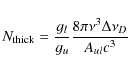
The column densities at which the 63 ![]() m line becomes optically thick can be approximated (
m line becomes optically thick can be approximated (
![]() ,
,
![]() ) as
) as
|
(11) |
where gu and gl are the statistical weights of the upper and lower level, Aul the Einstein A coefficient for the respective line transition with the frequency
The surface of the inner 30 AU of the
![]() disk model is very hot with gas temperatures of several thousand K and typical densities above 107 cm-3. Thus, the relative level populations with respect to the total oxygen number density
disk model is very hot with gas temperatures of several thousand K and typical densities above 107 cm-3. Thus, the relative level populations with respect to the total oxygen number density ![]() ,
in LTE, follow from the ratios of the statistical weights,
,
in LTE, follow from the ratios of the statistical weights,
![]() ,
,
![]() ,
,
![]() (see Table 3 for the notation - nJ with g=2J+1 being the statistical weight of the level). Under these physical circumstances, both O I lines become optically thick at column densities of
(see Table 3 for the notation - nJ with g=2J+1 being the statistical weight of the level). Under these physical circumstances, both O I lines become optically thick at column densities of ![]()
![]() cm-2.
Such column densities are reached inside 30 AU, even in our lowest
mass disk model. However, the contribution to the integrated line
emission from this hot gas is negligible. Removing the contribution
from hot gas by setting the O I abundance to zero for gas temperatures in excess of 2000 K, results in line flux changes that are less than 1%.
cm-2.
Such column densities are reached inside 30 AU, even in our lowest
mass disk model. However, the contribution to the integrated line
emission from this hot gas is negligible. Removing the contribution
from hot gas by setting the O I abundance to zero for gas temperatures in excess of 2000 K, results in line flux changes that are less than 1%.
In the 30-100 AU range, gas temperatures are much lower (few
hundred K) and only about 10% (3%) of the oxygen atoms reside in
the upper level of the 63 (145) ![]() m line. For those regions, the 145
m line. For those regions, the 145 ![]() m line becomes optically thin in the 10-3 and
m line becomes optically thin in the 10-3 and
![]() disk models. Emission from this ring dominates the total line emission.
We will get back to this point later. Models that include X-ray heating
and ionization (Nomura et al. 2007; Meijerink et al. 2008)
indicate that the impact of those additional processes is mostly
relevant inside 30 AU. Beyond that, UV processes dominate the gas
energy balance and chemistry. Hence, we do not expect X-rays to
significantly alter the [O I] line emission for disks with masses
disk models. Emission from this ring dominates the total line emission.
We will get back to this point later. Models that include X-ray heating
and ionization (Nomura et al. 2007; Meijerink et al. 2008)
indicate that the impact of those additional processes is mostly
relevant inside 30 AU. Beyond that, UV processes dominate the gas
energy balance and chemistry. Hence, we do not expect X-rays to
significantly alter the [O I] line emission for disks with masses
![]() .
In lower mass disks, the [O I] emission originates closer to the star and here X-rays could have an impact by increasing the gas temperatures.
.
In lower mass disks, the [O I] emission originates closer to the star and here X-rays could have an impact by increasing the gas temperatures.
The outer disk, beyond 100 AU, is fairly cold (
![]() K). Here, level population numbers of the J = 0 and J = 1 level are extremely small (below 0.5%). The peak separation
K). Here, level population numbers of the J = 0 and J = 1 level are extremely small (below 0.5%). The peak separation
![]() km s-1 of the [O I] 63
km s-1 of the [O I] 63 ![]() m line in the
m line in the
![]() disk model (see Fig. 7) indicates that the emission comes mostly from inside 380 AU; the [O I] 145
disk model (see Fig. 7) indicates that the emission comes mostly from inside 380 AU; the [O I] 145 ![]() m originates slightly closer to the star, inside 200 AU (
m originates slightly closer to the star, inside 200 AU (
![]() km s-1). The disk surface outside of 100 AU accounts for roughly 50% of the O I
emission. For the lowest mass disk model, the physical conditions in
this region such as gas/dust temperature and densities get close to
molecular cloud values of
km s-1). The disk surface outside of 100 AU accounts for roughly 50% of the O I
emission. For the lowest mass disk model, the physical conditions in
this region such as gas/dust temperature and densities get close to
molecular cloud values of
![]() K,
K,
![]() K,
K,
![]() cm-3.
cm-3.
In a series of radiative transfer calculations for the chemo-physical structure from the
![]() disk model, we studied the fraction of the emission coming from regions with densities above
disk model, we studied the fraction of the emission coming from regions with densities above
![]() .
Varying that density from the critical density of the 63
.
Varying that density from the critical density of the 63 ![]() m line,
m line,
![]() cm-3, to a density of 108 cm-3,
shows that the regions below the critical density do not contribute
very much to the total line emission. The emission gradually builds up
with increasing density, showing that the line originates from regions
up to an extinction of
cm-3, to a density of 108 cm-3,
shows that the regions below the critical density do not contribute
very much to the total line emission. The emission gradually builds up
with increasing density, showing that the line originates from regions
up to an extinction of
![]() .
.
![\begin{figure}
\par\includegraphics[width=18cm,clip]{13076fg4.eps}
\end{figure}](/articles/aa/full_html/2010/02/aa13076-09/img169.png)
|
Figure 4:
Departure coefficient
|
| Open with DEXTER | |
![\begin{figure}
\par\includegraphics[width=18cm]{13076fg5.eps}
\end{figure}](/articles/aa/full_html/2010/02/aa13076-09/img170.png)
|
Figure 5:
Departure coefficient
|
| Open with DEXTER | |
5.2.2 LTE versus escape probability versus Monte Carlo
LTE level population numbers systematically overestimate line fluxes by up to 70%. In the regions where most of the O I emission arises, the upper levels are significantly less populated than in LTE while the ground state is overpopulated with respect to LTE (Figs. 4 and 5). In the regions inside 30 AU, the H2 abundance is low, thus the main collision partners are atomic hydrogen and electrons. Outside 30 AU, hydrogen is predominantly in molecular form.
The level population numbers computed with the simple escape
probability assumption in ProDiMo yield only slightly higher line
fluxes, within 10% for the O I lines and ![]() 5%
higher continuum fluxes. Calculating the line emission from Monte-Carlo
radiative transfer requires a re-gridding of the ProDiMo model results.
Figure 6 shows the level population numbers of the 3P1 level of oxygen (upper level of the 63
5%
higher continuum fluxes. Calculating the line emission from Monte-Carlo
radiative transfer requires a re-gridding of the ProDiMo model results.
Figure 6 shows the level population numbers of the 3P1 level of oxygen (upper level of the 63 ![]() m
line) for two models. Differences arise mainly in the very optically
thin regions either at the disk surfaces or near the outer edge. In
these areas, the maximum escape probability following our two
directional escape probability approach is 0.5, while it should be
rather 1.0 in very optically thin environments. Hence, in those
areas the Monte Carlo approach gives a better result.
m
line) for two models. Differences arise mainly in the very optically
thin regions either at the disk surfaces or near the outer edge. In
these areas, the maximum escape probability following our two
directional escape probability approach is 0.5, while it should be
rather 1.0 in very optically thin environments. Hence, in those
areas the Monte Carlo approach gives a better result.
Since continuum differences should largely be due to the re-gridding,
the estimated error stemming from the interpolation onto a different
grid is of the order of 5%. Considering that, the intrinsic difference
in line fluxes of both line radiative transfer methods is fairly small.
The visible differences in the level population numbers are largest in
the regions that do not contribute significantly to the total line
emission (well above the critical density iso-contour in Fig. 6), i.e. the very tenuous surface and outer (![]() AU) regions of the disk.
AU) regions of the disk.
![\begin{figure}
\par\includegraphics[width=9cm,clip]{13076fg6.eps}
\end{figure}](/articles/aa/full_html/2010/02/aa13076-09/img174.png)
|
Figure 6:
O I 3P1 level population numbers from A MC,
|
| Open with DEXTER | |
![\begin{figure}
\par\includegraphics[width=18cm]{13076fg7.eps}
\end{figure}](/articles/aa/full_html/2010/02/aa13076-09/img175.png)
|
Figure 7:
Top row: [O I] 63 |
| Open with DEXTER | |
5.3 CO sub-mm lines
![\begin{figure}
\par\begin{tabular}{ccc}
\hspace*{-10mm}\includegraphics[height=...
...ight=5.0cm]{13076fg16.eps} \end{tabular}\\ *[-1mm]\vspace*{-2mm}
\end{figure}](/articles/aa/full_html/2010/02/aa13076-09/img176.png)
|
Figure 8: The top row shows integrated line fluxes as a function of disk mass, for ( from left to right) the CO J=1-0, J=2-1 and J=3-2 rotational lines. The second row shows the continuum fluxes at the corresponding line center wavelengths as a function of disk mass. The third row shows the CO line ratios as a function of disk mass: ( from left to right) J=2-1/1-0, J=3-2/1-0, J=3-2/2-1. Dashed lines indicate computed line ratios for optically thick lines in LTE. |
| Open with DEXTER | |
Line fluxes have been calculated for the first three molecular transitions in CO, across the full mass range of disk models. The line fluxes and continuum fluxes are plotted as a function of disk mass in Fig. 8.
The J=1-0, J=2-1 and J=3-2 lines all show similar behaviour with disk
mass, with the line fluxes initially increasing sharply with mass
before levelling off for
![]() .
This
similarity results in largely uniform line ratios, with a spike at
.
This
similarity results in largely uniform line ratios, with a spike at
![]() .
The continuum varies almost linearly with disk
(and hence dust) mass, although with slightly more emission from the lower mass models
than a strict linear relationship would give. This is due to the
optically thin low mass disks having more penetrating UV dust heating
in the midplane than the higher mass optically thick disks.
.
The continuum varies almost linearly with disk
(and hence dust) mass, although with slightly more emission from the lower mass models
than a strict linear relationship would give. This is due to the
optically thin low mass disks having more penetrating UV dust heating
in the midplane than the higher mass optically thick disks.
The calulated line fluxes all exhibit a jump of four orders of
magnitude on moving from the 10-5 to the
![]() model. This discontinuity is also seen in the line ratios, with all
three exhibiting a significantly higher ratio for the
model. This discontinuity is also seen in the line ratios, with all
three exhibiting a significantly higher ratio for the
![]() model than for the others. The sudden drop in emission below
model than for the others. The sudden drop in emission below
![]() corresponds to a fall-off in AV. There is suddenly almost no region
in the disk with AV > 0.1, resulting in a maximum CO abundance of
less than 10-6 compared with
corresponds to a fall-off in AV. There is suddenly almost no region
in the disk with AV > 0.1, resulting in a maximum CO abundance of
less than 10-6 compared with ![]() 10-4 for the higher mass
models. The small remaining region with AV > 0.1 is quite hot,
with gas temperatures around 500 K, giving a spike in the line ratios at
10-4 for the higher mass
models. The small remaining region with AV > 0.1 is quite hot,
with gas temperatures around 500 K, giving a spike in the line ratios at
![]() .
.
5.3.1 Line formation regions
The three CO lines form at an intermediate height in the disk, between
the warm upper layer and the cold midplane (see also van Zadelhoff et al. 2001) and are generally optically thick for disk masses down to
![]() .
The submm line formation
region is radially very extended, with significant contributions to the total line
flux from the entire disk. The results of an experiment varying the
outer radius of the disk region sampled in the re-gridding procedure
are plotted in Fig. 9. The total J=3-2 line flux is seen to
vary linearly with
.
The submm line formation
region is radially very extended, with significant contributions to the total line
flux from the entire disk. The results of an experiment varying the
outer radius of the disk region sampled in the re-gridding procedure
are plotted in Fig. 9. The total J=3-2 line flux is seen to
vary linearly with
![]() indicating that the line
originates from the full radial extent of the disk. The same behaviour
is seen in the J=1-0 and J=2-1 lines. The linear trend is caused by a combination of the radial
gas temperature gradient in the CO emitting layers and surface area. The continuum shows a slightly different
behaviour, with a greater proportion of the integrated flux from outer
radii.
indicating that the line
originates from the full radial extent of the disk. The same behaviour
is seen in the J=1-0 and J=2-1 lines. The linear trend is caused by a combination of the radial
gas temperature gradient in the CO emitting layers and surface area. The continuum shows a slightly different
behaviour, with a greater proportion of the integrated flux from outer
radii.
The line profiles for the three transitions are generally very similar
for a given disk model, and indeed across the computed mass range.
Narrow peak
separations (
![]() km s-1) indicate that the emission is coming from the entire disk inside
km s-1) indicate that the emission is coming from the entire disk inside ![]() 700 AU and will thus be dominated by the outer regions that
contain more surface area.
700 AU and will thus be dominated by the outer regions that
contain more surface area.
5.3.2 LTE versus escape probability versus Monte Carlo
The continuum results obtained without re-gridding (ES) are in good
agreement with those from the Monte Carlo radiative transfer,
within 3% in all cases. This indicates that re-gridding does not
present an issue when considering sub-mm fluxes. The escape probability
line fluxes deviate slightly from the Monte Carlo and LTE fluxes for
the low disk masses, up to ![]() 50%
lower. This indicates again the limits of the two direction escape
probability approach for the optically thin case of very tenuous disks.
50%
lower. This indicates again the limits of the two direction escape
probability approach for the optically thin case of very tenuous disks.
The escape probability fluxes are however in good agreement (within 3%) for disk models with masses larger than
![]() .
The LTE line fluxes are also in good agreement (within
.
The LTE line fluxes are also in good agreement (within ![]() 1%) for the entire mass range (see Fig. 10), indicating that LTE is a valid approximation for these low CO lines. However,
1%) for the entire mass range (see Fig. 10), indicating that LTE is a valid approximation for these low CO lines. However,
![]() is not a valid approximation for this set of disk models, because the
gas temperatures in the outer regions, where the CO lines arise,
deviate by up to a factor two from the dust temperatures (see
Table 4 for mass averaged gas and dust temperatures of CO).
is not a valid approximation for this set of disk models, because the
gas temperatures in the outer regions, where the CO lines arise,
deviate by up to a factor two from the dust temperatures (see
Table 4 for mass averaged gas and dust temperatures of CO).
5.3.3 CO line ratios
To understand the values of the CO line ratios for high mass disks in Fig. 8, we start with a number of assumptions: 1) the continuum is small
![]() ;
2) the CO line forms under optically thick LTE conditions with a universal line profile
;
2) the CO line forms under optically thick LTE conditions with a universal line profile ![]() such that
such that
![]() where
where ![]() is the Planck function; 3) the temperature
is the Planck function; 3) the temperature
![]() is constant throughout the line forming region. The line flux can then be expressed as
is constant throughout the line forming region. The line flux can then be expressed as
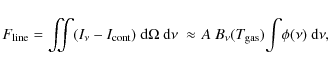
where A is the disk surface area as seen by the observer.
![\begin{figure}
\par\includegraphics[width=9cm,clip]{13076fg17.eps}
\end{figure}](/articles/aa/full_html/2010/02/aa13076-09/img185.png)
|
Figure 9:
Integrated CO J=3-2 line flux for the
|
| Open with DEXTER | |
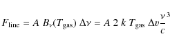
If we assume a square line profile function in velocity space such that
![]() if
if
![]() and
and
![]() otherwise, we can re-write Eq. (12) in the Rayleigh-Jeans limit as
otherwise, we can re-write Eq. (12) in the Rayleigh-Jeans limit as
|
(13) |
using

|
(14) |
The corresponding values for the three CO line ratios are overplotted with dashed lines on Fig. 8, and agree indeed well with the limiting behaviour of the line ratios at high disk masses,
Changing the effective temperature of the central star or changing
the dust properties affects the CO lines to a lesser extent than the
fine structure lines. Changes to the continuum and the lines are
generally within 50%. Even though the formation height of CO might
change slightly, the excitation conditions are still close to LTE.
While the CO mass in the models stays within a few percent of the
original model (except in the ISM grain model, where it is 26% smaller)
the CO mass averaged temperature changes up to a factor two. The effect
on the line fluxes correlates directly with the temperature change,
with the higher temperatures giving systematically higher fluxes. At
these radio wavelengths, the change in continuum emission amounts to
less than 25%, even between the models with different dust properties.
The most extreme model is the one with an effective temperature of
10 500 K where the mass averaged CO temperature rises to
110 K and hence the line fluxes increase by ![]() 60-70%.
60-70%.
6 Discussion
The goal of this study is a first assessment of the diagnostic power of the fine structure lines of neutral oxygen, ionized carbon and of the CO submm lines in protoplanetary disks. This work prepares the ground for a systematic analysis of a much larger and more complete grid of protoplanetary disk models. Based on the detailed radiative transfer calculations of the previous section, we discuss here the potential of the various lines in the context of deriving physical disk properties such as gas mass, gas temperatures and disk extension.
6.1 [O I] 63 line
Using one dimensional modeling of photon-dominated regions (PDRs), Liseau et al. (2006) find that the total intensity of the 63 ![]() m
line can be used as an indicator of the gas temperature in outflows
from young stellar objects. From detailed two dimensional modeling of
protoplanetary disks, Woitke et al. (2009a) conclude that the [O I] 63
m
line can be used as an indicator of the gas temperature in outflows
from young stellar objects. From detailed two dimensional modeling of
protoplanetary disks, Woitke et al. (2009a) conclude that the [O I] 63 ![]() m
line alone will indeed provide a useful tool to deduce the gas
temperature in the surface layers of protoplanetary disks, especially
the hot inner disk surface. However, spatially unresolved observations
that measure only integrated [O I] 63
m
line alone will indeed provide a useful tool to deduce the gas
temperature in the surface layers of protoplanetary disks, especially
the hot inner disk surface. However, spatially unresolved observations
that measure only integrated [O I] 63 ![]() m
line fluxes in sources at typical distances of 140 pc will not be
able to detect the presence of hot gas very close to the star (inside
m
line fluxes in sources at typical distances of 140 pc will not be
able to detect the presence of hot gas very close to the star (inside ![]() 10 AU). The total line flux is dominated by emission coming from the cooler outer regions (Table 5).
10 AU). The total line flux is dominated by emission coming from the cooler outer regions (Table 5).
6.2 [O I] 63/145 line ratio
The diagnostic power of the [O I] 63/145 ![]() m line ratio has been discussed by Tielens & Hollenbach (1985) for PDRs and by Liseau et al. (2006)
for outflows around young stellar objects (YSOs). Very low ratios of a
few can be explained if both lines are optically thick (see Fig. 2
of Tielens & Hollenbach 1985). In that case the diagnostic power of this line ratio is very limited. Liseau et al. (2006)
find that even in the optically thin limit, the line ratio can be
degenerate with low temperature molecular gas giving the same result as
high temperature atomic gas. This is due to the different collisional
cross sections for O-H and O-H2. From ISO observations, Lorenzetti et al. (2002)
found ratios between 2 and 10 for Herbig Ae/Be stars. They derive from
PDR modeling of a clumpy medium that the low line ratios of a few would
require very high column densities of
m line ratio has been discussed by Tielens & Hollenbach (1985) for PDRs and by Liseau et al. (2006)
for outflows around young stellar objects (YSOs). Very low ratios of a
few can be explained if both lines are optically thick (see Fig. 2
of Tielens & Hollenbach 1985). In that case the diagnostic power of this line ratio is very limited. Liseau et al. (2006)
find that even in the optically thin limit, the line ratio can be
degenerate with low temperature molecular gas giving the same result as
high temperature atomic gas. This is due to the different collisional
cross sections for O-H and O-H2. From ISO observations, Lorenzetti et al. (2002)
found ratios between 2 and 10 for Herbig Ae/Be stars. They derive from
PDR modeling of a clumpy medium that the low line ratios of a few would
require very high column densities of
![]() cm-3 (
cm-3 (
![]() mag)
and conclude that better models of the emitting region are required for
the physical interpretation of this data. Studying the outflows of
several hundred YSOs with ISO, Liseau et al. (2006) found [O I] 63/145
mag)
and conclude that better models of the emitting region are required for
the physical interpretation of this data. Studying the outflows of
several hundred YSOs with ISO, Liseau et al. (2006) found [O I] 63/145 ![]() m line ratios between
m line ratios between ![]() 1 and 50. They suggest that confusion with relatively cool but optically thick envelope gas (T < 100 K) could explain the low line ratio in some cases.
1 and 50. They suggest that confusion with relatively cool but optically thick envelope gas (T < 100 K) could explain the low line ratio in some cases.
![\begin{figure}
\par\includegraphics[width=7.6cm,clip]{13076fg18.eps}
\end{figure}](/articles/aa/full_html/2010/02/aa13076-09/img196.png)
|
Figure 10: Relative difference in percent between Monte Carlo CO line fluxes and CO line fluxes calculated using the escape probabilty assumption (solid line) and between Monte Carlo CO line fluxes and LTE CO line fluxes (dotted line); results are shown as a function of disk mass. |
| Open with DEXTER | |
Figure 11 shows that the [O I] 63/145 line ratio increases towards lower masses (10 for ![]()
![]() to 40 for
to 40 for
![]() ).
Our line ratio for massive disks corresponds well to the expected value
for both lines being optically thick and arising from relatively warm
gas, T > 100 K, that resides in the surface layers of
the disk. As the disk mass decreases, first the 145 and then the
63
).
Our line ratio for massive disks corresponds well to the expected value
for both lines being optically thick and arising from relatively warm
gas, T > 100 K, that resides in the surface layers of
the disk. As the disk mass decreases, first the 145 and then the
63 ![]() m line become optically thin. Eventually, the optically thin limit is reached for disk masses smaller than
m line become optically thin. Eventually, the optically thin limit is reached for disk masses smaller than
![]() ,
leading to line ratios of
,
leading to line ratios of ![]() 40.
In a simple one dimensional model, this corresponds to gas temperatures
in excess of 100 K and a wide range of densities. The line
profiles show an increasing peak separation towards lower mass disks
(see Fig. 7). In fact, the line emission in low mass disks is dominated by disk material close to the star (r<100 AU), while in high mass disks, the emission comes from the disk surface out to
40.
In a simple one dimensional model, this corresponds to gas temperatures
in excess of 100 K and a wide range of densities. The line
profiles show an increasing peak separation towards lower mass disks
(see Fig. 7). In fact, the line emission in low mass disks is dominated by disk material close to the star (r<100 AU), while in high mass disks, the emission comes from the disk surface out to ![]() 200 AU and is hence dominated by the outer regions (
30 < r < 200 AU). The sequence of the
200 AU and is hence dominated by the outer regions (
30 < r < 200 AU). The sequence of the
![]() disk model with varying outer radii (dotted line in Fig. 11) shows that the [O I] 63/145
line ratio is indeed not sensitive to the disk outer radius unless the
disk starts to become smaller than the region where most emission
originates (see the
disk model with varying outer radii (dotted line in Fig. 11) shows that the [O I] 63/145
line ratio is indeed not sensitive to the disk outer radius unless the
disk starts to become smaller than the region where most emission
originates (see the
![]() AU model).
AU model).
The effective temperature and thus amount of UV radiation from the
central star has a negligible impact on the line ratio in the
temperature range of Herbig Ae stars. Both lines increase by the same
amount (up to a factor 7 for the individual line fluxes for
![]() K compared to the standard case of
K compared to the standard case of
![]() K)
due to the overall warmer gas temperatures (the oxygen mass does not
change by more than 5%). The change in line ratio due to a factor
10 decrease in disk mass is much larger than the change due to a
different effective temperature of the star.
K)
due to the overall warmer gas temperatures (the oxygen mass does not
change by more than 5%). The change in line ratio due to a factor
10 decrease in disk mass is much larger than the change due to a
different effective temperature of the star.
On the other hand, the grain size distribution does have a larger effect on the line ratios as expected from the impact on the disk structure (see Sect. 4.5). The line ratio is 10% smaller for the disk model with large micron sized dust grains. Using only small sub-micron sized grains (similar to the ISM composition) increases the line ratio by a factor two, thus mimicking a disk mass that is lower by more than a factor ten. Since the disk with small ISM grains is flatter and reaches thus higher particle densities, O depletes more readily into species such as water and water ice, hence decreasing the overall vertical column density of neutral oxygen (making the lines thus marginally optically thin). However, the grain size distributions chosen here present the extreme ends and are easily distinguished from looking at the SED.
The typical hydrogen number densities in the emitting region range up to 108 cm-3,
higher than those generally covered in PDR models (even in clumpy
PDRs). The vertical column density of neutral oxygen reaches values of
1020 cm-3 and temperatures above 200 K inside 10 AU and 1019 cm-3 and temperatures below 100 K in the outer disk (
![]() disk model). The large difference to PDR conditions can explain the problems and high extinction values that Lorenzetti et al. (2002)
found from their classical PDR analysis. However, our highest mass disk
models do not show line ratios as low as 2, the most extreme cases
of the YSOs studied by Liseau et al. (2006). For embedded objects, confusion with relatively cool but optically thick envelope gas (T < 100 K) is still a viable explanation of the low ratios.
disk model). The large difference to PDR conditions can explain the problems and high extinction values that Lorenzetti et al. (2002)
found from their classical PDR analysis. However, our highest mass disk
models do not show line ratios as low as 2, the most extreme cases
of the YSOs studied by Liseau et al. (2006). For embedded objects, confusion with relatively cool but optically thick envelope gas (T < 100 K) is still a viable explanation of the low ratios.
![\begin{figure}
\par\includegraphics[width=8cm]{13076fg19.ps}
\end{figure}](/articles/aa/full_html/2010/02/aa13076-09/img201.png)
|
Figure 11:
[O I] 63/145 |
| Open with DEXTER | |
6.3 [C II] 158 m line
The [C II] 158 ![]() m line emission is a very sensitive tracer of the outer disk radius. We come back to this point in Sect. 6.5. As expected, the integrated line flux from our models scales as
m line emission is a very sensitive tracer of the outer disk radius. We come back to this point in Sect. 6.5. As expected, the integrated line flux from our models scales as
![]() .
This makes it more difficult to detect smaller size disks that are only of the order of 100 AU in size.
.
This makes it more difficult to detect smaller size disks that are only of the order of 100 AU in size.
Due to its low excitation temperature, this line is also
strongly affected by confusion with any type of diffuse and molecular
cloud material in the line of sight. The problem can be addressed with
Herschel/PACS by using the surrounding pixels on the detector (
![]() pixels with the disk being spatially unresolved) for a reliable off-source flux determination.
pixels with the disk being spatially unresolved) for a reliable off-source flux determination.
Changing the dust properties to very large grains results in a much lower [C II] 158 ![]() m line flux, the reason being that above the
m line flux, the reason being that above the
![]() layer
outside of 100 AU, the gas temperature drops below the excitation
temperature for this line. The gas inside 30 AU becomes much
warmer due to the gas-dust de-coupling, thereby generating a more
pronounced secondary rim. This casts an efficient shadow on the outer
disk, thereby enhancing the CO formation (H2 and CO self-shielding) and thus the molecular line cooling.
layer
outside of 100 AU, the gas temperature drops below the excitation
temperature for this line. The gas inside 30 AU becomes much
warmer due to the gas-dust de-coupling, thereby generating a more
pronounced secondary rim. This casts an efficient shadow on the outer
disk, thereby enhancing the CO formation (H2 and CO self-shielding) and thus the molecular line cooling.
6.4 [O I] 63/[C II] 158 line ratio
The [O I] 63/[C II] 158 ratio depends even more on disk mass than the [O I] 63/145
line ratio. It would thereby be a prime diagnostic for relative disk
mass estimates. However, while the ratio of the two oxygen lines does
not change very much with disk outer radius, the [O I] 63/[C II] 158 ratio does depend strongly on it (Fig. 12). The
![]() disk model with an outer radius of 100 AU has a more than 10 times higher [O I] 63/[C II] 158 line ratio than the same model with an outer radius of 700 AU.
disk model with an outer radius of 100 AU has a more than 10 times higher [O I] 63/[C II] 158 line ratio than the same model with an outer radius of 700 AU.
Because of this degeneracy with disk size, the diagnostic value of this ratio alone is limited for individual objects. Its use would require the a-priori knowledge of many other disk parameters such as the disk outer radius, grain sizes and composition. Rather we suggest that it could be used in a statistical way on a large sample of disks that share the same classification group, e.g. based on their IR SEDs. Alternatively, a combination of the [O I] 63/145 and [O I] 63/[C II] 158 line ratios could be used to break the degeneracy with disk size. Figure 13 shows clearly that disks with a smaller outer radius, e.g. 300 AU, lie well to the right of the standard relation, while the presence of an inner hole for example (30 AU size here) does not affect the location in this diagnostic diagram.
As for the oxygen fine structure line ratio, the [O I] 63/ [C II] 158 ratio depends strongly on the chosen grain size distribution. Additional SED observations are required to constrain the dust parameters to a reasonable range. It is important to note that the change in line ratios in the [O I] 63/145 versus [O I] 63/[C II] 158 plot has a direction different from what we expect from a change in disk mass. Also, the [O I] 63/[C II] 158 ratio is less sensitive to the effective temperature of the star than it is to disk mass.
![\begin{figure}
\par\includegraphics[width=7.5cm,clip]{13076fg20.ps}
\end{figure}](/articles/aa/full_html/2010/02/aa13076-09/img204.png)
|
Figure 12:
[O I] 63/[C II] 158 |
| Open with DEXTER | |
![\begin{figure}
\par\includegraphics[width=8cm,clip]{13076fg21.ps}
\end{figure}](/articles/aa/full_html/2010/02/aa13076-09/img205.png)
|
Figure 13:
[O I] 63/145 |
| Open with DEXTER | |
6.5 CO submm lines and line ratios
The low excitation CO rotational lines are often used to prove the existence of primordial gas in protoplanetary disk and in combination with optically thin line of isotopologues to measure the total gas mass (e.g. Thi et al. 2001; Panic et al. 2008). Due to the high Einstein A coefficients and high abundances of 12CO in molecular regions, the low rotational CO lines become optically thick at low AV. Thus, they originate mainly in the optically thin disk surface (van Zadelhoff et al. 2001), where gas and dust temperature decouple according to our models. However, as in the case of the [C II] line, CO submm lines can be contaminated by low density cold remnant cloud material. The amount of contamination can be estimated either from offset positions for single dish observations or through interferometry.
Isotopologues of CO have much lower abundances of 12CO/13CO =77 in the ISM (Wilson & Rood 1994) and even higher values of 100 in disks (selective photodissociation; see for most recent work Woods & Willacy 2009; Visser et al. 2009; Smith et al. 2009).
Thus, they can probe deeper into the disk and are - in the absence of
freeze-out - excellent tools for measuring the disk mass. Panic et al. (2008) use for example the optically thin 13CO J=2-1 line from the disk around the Herbig star HD 169142 to infer a disk mass of
![]() .
.
Our analysis shows indeed a relatively flat relationship for the 12CO lines with disk gas mass, confirming thus that the low rotational CO lines by themselves are not a good tracer of gas mass (Fig. 8). The lines become optically thick even at very low disk masses and hence a reliable inversion of the line fluxes to infer gas mass proves impossible. Similarly there are degeneracies in the computed line ratios J = 2-1/1-0, J=3-2/1-0 and J=3-2/2-1 which suggest limitations in the diagnostic power of these line ratios.
The CO lines can be used to measure independently the outer disk radius (Sect. 5.3.1) and thus mitigate the problem of employing the [C II] 158 line for disk diagnostics. Dent et al. (2005) and Panic & Hogerheijde (2009)
demonstrate the power of single dish CO observations in deriving disk
outer radii and inclinations, thus constraining SED modeling that is
rather insensitive to
![]() and degenerate for inclination and inner radius. Hughes et al. (2008b)
note that the outer radius derived from dust continuum observations is
always smaller than that derived from CO emission lines. Even though
they can explain this within homogeneous gas and dust models (
and degenerate for inclination and inner radius. Hughes et al. (2008b)
note that the outer radius derived from dust continuum observations is
always smaller than that derived from CO emission lines. Even though
they can explain this within homogeneous gas and dust models (
![]() and
a realistic outer edge, i.e. an exponential density profile), this
finding reveals the problems in mixing quantities deduced from dust and
gas observations. Since C+
and CO arise both from the gas in the outer disk, we do not need to
rely on dust observations, but can instead use a gas tracer to measure
the gas outer disk radius.
and
a realistic outer edge, i.e. an exponential density profile), this
finding reveals the problems in mixing quantities deduced from dust and
gas observations. Since C+
and CO arise both from the gas in the outer disk, we do not need to
rely on dust observations, but can instead use a gas tracer to measure
the gas outer disk radius.
The [C II] line probes in general
slightly higher layers than the CO lines; hence the model results
suggest that we can trace the vertical gas temperature gradient in
disks. Table 4 shows that for the most massive disks,
![]() is 50% larger than
is 50% larger than
![]() .
.
6.6 Comparison with observations for MWC480
Since we used the Herbig star MWC480 to motivate our choice of
parameters, we briefly discuss the line emission from the models
together with observations available from the literature. The goal is
not to obtain a best-fitting model, but to provide an impression of the
model results within the observational context. Table 6
gives an overview of selected observational data for MWC480 (detections
and upper limits) from the literature. The CO mass derived from 13CO 3-2 is
![]() and the total gas mass derived from the 1.3 mm continuum flux is
and the total gas mass derived from the 1.3 mm continuum flux is
![]() (Thi et al. 2001). The 12CO and 13CO lines suggest an outer disk radius of
(Thi et al. 2001). The 12CO and 13CO lines suggest an outer disk radius of ![]() 750 and
750 and ![]() 500 AU, respectively (Piétu et al. 2007).
500 AU, respectively (Piétu et al. 2007).
The oxygen fine structure lines are not detected with the ISO satellite (Creech-Eakman et al. 2002). Assuming the ISO instrumental resolution as FWHM of a potential line (0.3 ![]() m for
m for
![]() m, 0.6
m, 0.6 ![]() m for
m for
![]() m), the ISO 3
m), the ISO 3![]() upper limits for the [O I] lines can be derived from
upper limits for the [O I] lines can be derived from
|
(15) |
This gives values of
The observed [C II] line is much stronger than in any of our models, suggesting indeed significant contamination from diffuse background material in the large ISO beam (80'').
Our
![]() model overpredicts the CO J=3-2
line flux by approximately one order of magnitude. By reducing the
maximum grain size, the total grain surface area increases and dust and
gas temperatures couple in the region where this CO line forms; thus
yielding
model overpredicts the CO J=3-2
line flux by approximately one order of magnitude. By reducing the
maximum grain size, the total grain surface area increases and dust and
gas temperatures couple in the region where this CO line forms; thus
yielding
![]() K
and a factor two lower line fluxes. Another factor two can each be
gained by reducing the total disk mass and the disk outer radius to 500
instead of 700 AU.
K
and a factor two lower line fluxes. Another factor two can each be
gained by reducing the total disk mass and the disk outer radius to 500
instead of 700 AU.
The observed continuum flux at 1.3 mm is a factor 4 smaller than computed from the
![]() disk
model. Reducing again either the total disk mass or the maximum grain
size, reduces the modeled continuum fluxes to the right value.
disk
model. Reducing again either the total disk mass or the maximum grain
size, reduces the modeled continuum fluxes to the right value.
To conclude, by tuning the input parameters, the models can get close to the observed continuum as well as line fluxes, thus providing additional confidence that the models capture the essential physics and chemistry of protoplanetary disks. Hence, besides studying physics and chemistry of protoplanetary disks in a more general context, these models can also be used in the detailed analysis of individual objects that possess a larger set of continuum and line observations.
Table 6: Observed fluxes for MWC480.
7 Conclusions
We used here a limited series of Herbig Ae disk models computed with the new thermo-chemical disk code called P ROD IM O to study the origin and diagnostic value of the gas line tracers [C II], [O I] and CO. We do not include in this study effects of X-ray irradiation, grain settling or mixing. Even though X-rays are generally of minor importance for Herbig stars, grain settling and large scale mixing processes could affect the conclusions. The effect of grain settling will be included in a forthcoming larger model grid, but mixing processes need to be addressed with dynamical time-dependant models. The Monte-Carlo radiative transfer code R ATRAN is used to compute line profiles and integrated emission from various gas lines.
The main results are:
- The [C II] line originates in the disk surface
layer where gas and dust temperatures are decoupled. The total line
strength is dominated by emission from the disk outer radius. Thus the
157.7 m line probes mainly the disk extension and outer disk gas temperature. The line forms in LTE.
- The [O I] lines originate also in the disk surface layer even though somewhat deeper than the [C II] line. The main contribution comes from radii between 30 and 100 AU. The [O I] lines form partially under NLTE conditions. Differences in line emission from escape probability and Monte Carlo techniques are smaller than 10%.
- CO submm lines are optically thick down to very low disk masses of <
 and form mostly in LTE.
 is
not a valid approximation for these lines. Differences in line emission
from escape probability and Monte Carlo techniques are smaller than 3%,
except in the case of very optically thin disk models (10-5 and
is
not a valid approximation for these lines. Differences in line emission
from escape probability and Monte Carlo techniques are smaller than 3%,
except in the case of very optically thin disk models (10-5 and
 ).
).
- The [O I] 63/145 m and [O I] 63/[C II] 158 m line ratios trace disk mass in the regime between 10-2 and
.
Since the [C II] 158 m line is very sensitive to the outer disk radius, the [O I] 63/[C II] 158 m
is degenerate in that respect and its use requires additional
constraints from ancilliary gas and/or dust observations. The
sensitivity of these two line ratios to the dust grain sizes underlines
the importance of using SED constraints along with the gas modeling to
mitigate the uncertainty of dust properties.
- A combination of the [O I] 63/145 m and [O I] 63/ [C II] 158 m line ratios can be used to diminish the degeneracy caused by an unknown outer disk radius.
- Neither total CO submm line fluxes nor line ratios can be used
to measure the disk mass. However, the low rotational lines studied
here provide an excellent tool to measure the disk outer radius and can
thus help to mitigate the degeneracy between gas mass and outer radius
found for the [O I] 63/[C II] 158 m line ratio.
We thank Dieter Poelman for fruitful discussions about radiative transfer methods and detailed code comparisons.
References
- Auer, L. 1984, in Numerical Radiative Transfer, ed. W. Kalkhofen (Cambridge: Cambridge Univ. Press), 101 [Google Scholar]
- Beckwith, S., Sargent, A. I., Scoville, N. Z., et al. 1986, ApJ, 309, 755 [NASA ADS] [CrossRef] [Google Scholar]
- Beckwith, S. V. W., & Sargent, A. I. 1991, ApJ, 381, 250 [NASA ADS] [CrossRef] [Google Scholar]
- Bell, K. L., Berrington, K. A., & Thomas, M. R. J. 1998, MNRAS, 293, L83 [NASA ADS] [CrossRef] [Google Scholar]
- Bratley, P., Fox, B. L., & Niederreiter, H. 1994, ACM Transactions on Mathematical Software, 20, 494 [CrossRef] [Google Scholar]
- Brott, I., & Hauschildt, P. H. 2005, in The Three-Dimensional Universe with Gaia, ed. C. Turon, K. S. O'Flaherty, & M. A. C. Perryman, ESA SP-576, 565 [Google Scholar]
- Chu, S.-I., & Dalgarno, A. 1975, R. Soc. London Proc. Ser. A, 342, 191 [Google Scholar]
- Creech-Eakman, M. J., Chiang, E. I., Joung, R. M. K., Blake, G. A., & van Dishoeck, E. F. 2002, A&A, 385, 546 [NASA ADS] [CrossRef] [EDP Sciences] [Google Scholar]
- Dartois, E., Dutrey, A., & Guilloteau, S. 2003, A&A, 399, 773 [NASA ADS] [CrossRef] [EDP Sciences] [Google Scholar]
- Dent, W. R. F., Greaves, J. S., & Coulson, I. M. 2005, MNRAS, 359, 663 [NASA ADS] [CrossRef] [Google Scholar]
- Draine, B. T., & Lee, H. M. 1984, ApJ, 285, 89 [Google Scholar]
- Dutrey, A., Guilloteau, S., & Guelin, M. 1997, A&A, 317, L55 [NASA ADS] [Google Scholar]
- Flower, D. R., & Launay, J. M. 1977, J. Phys. B Atom. Mol. Phys., 10, 3673 [NASA ADS] [CrossRef] [Google Scholar]
- Hickernell, F. J., & Yue, R.-X. 2000, SIAM J. Numer. Anal., 38, 1089 [CrossRef] [Google Scholar]
- Hogerheijde, M. R., & van der Tak, F. F. S. 2000, A&A, 362, 697 [NASA ADS] [Google Scholar]
- Hughes, A. M., Wilner, D. J., Kamp, I., et al. 2008a, ApJ, 681, 626 [NASA ADS] [CrossRef] [Google Scholar]
- Hughes, A. M., Wilner, D. J., Qi, C., et al. 2008b, ApJ, 678, 1119 [NASA ADS] [CrossRef] [Google Scholar]
- Isella, A., Testi, L., Natta, A., et al. 2007, A&A, 469, 213 [CrossRef] [EDP Sciences] [Google Scholar]
- Jaquet, R., Staemmler, V., Smith, M. D., et al. 1992, J. Phys. B Atom. Mol. Phys., 25, 285 [Google Scholar]
- Jonkheid, B., Dullemond, C. P., Hogerheijde, M. R., et al. 2007, A&A, 463, 203 [NASA ADS] [CrossRef] [EDP Sciences] [Google Scholar]
- Juvela, M. 1997, A&A, 322, 943 [NASA ADS] [Google Scholar]
- Kamp, I., Dullemond, C. P., Hogerheijde, M., et al. 2005, in Astrochemistry: Recent Successes and Current Challenges, ed. D. C. Lis, G. A. Blake, & E. Herbst, IAU Symp., 231, 377 [Google Scholar]
- Kamp, I., & van Zadelhoff, G.-J. 2001, A&A, 373, 641 [NASA ADS] [CrossRef] [EDP Sciences] [Google Scholar]
- Koerner, D. W., Sargent, A. I., & Beckwith, S. V. W. 1993, Icarus, 106, 2 [NASA ADS] [CrossRef] [Google Scholar]
- Launay, J. M., & Roueff, E. 1977, A&A, 56, 289 [NASA ADS] [Google Scholar]
- Liseau, R., Justtanont, K., & Tielens, A. G. G. M. 2006, A&A, 446, 561 [NASA ADS] [CrossRef] [EDP Sciences] [Google Scholar]
- Lorenzetti, D., Giannini, T., Nisini, B., et al. 2002, A&A, 395, 637 [NASA ADS] [CrossRef] [EDP Sciences] [Google Scholar]
- Mannings, V., & Emerson, J. P. 1994, MNRAS, 267, 361 [NASA ADS] [Google Scholar]
- Mannings, V., Koerner, D. W., & Sargent, A. I. 1997, Nature, 388, 555 [NASA ADS] [CrossRef] [PubMed] [Google Scholar]
- Mannings, V., & Sargent, A. I. 1997, ApJ, 490, 792 [NASA ADS] [CrossRef] [Google Scholar]
- Meijerink, R., Glassgold, A. E., & Najita, J. R. 2008, ApJ, 676, 518 [NASA ADS] [CrossRef] [Google Scholar]
- Niederreiter, H. 1992, Random number generation and quasi-Monte Carlo methods (Philadelphia, PA, USA: Society for Industrial and Applied Mathematics) [Google Scholar]
- Nomura, H., Aikawa, Y., Tsujimoto, M., Nakagawa, Y., & Millar, T. J. 2007, ApJ, 661, 334 [NASA ADS] [CrossRef] [Google Scholar]
- Ossenkopf, V., & Henning, T. 1994, A&A, 291, 943 [NASA ADS] [Google Scholar]
- Owen, A. B. 2003, ACM Trans. Model. Comput. Simul., 13, 363 [CrossRef] [Google Scholar]
- Panic, O., & Hogerheijde, M. R. 2009, A&A, 508, 707 [NASA ADS] [CrossRef] [EDP Sciences] [Google Scholar]
- Panic, O., Hogerheijde, M. R., Wilner, D., et al. 2008, A&A, 491, 219 [NASA ADS] [CrossRef] [EDP Sciences] [Google Scholar]
- Piétu, V., Guilloteau, S., & Dutrey, A. 2005, A&A, 443, 945 [NASA ADS] [CrossRef] [EDP Sciences] [Google Scholar]
- Piétu, V., Dutrey, A., & Guilloteau, S. 2007, A&A, 467, 163 [NASA ADS] [CrossRef] [EDP Sciences] [Google Scholar]
- Press, W. H., Teukolsky, S. A., Vetterling, W. T., et al. 2002, Numerical recipes in C++ : the art of scientific computing (Cambridge University Press) [Google Scholar]
- Rodmann, J., Henning, T., Chandler, C. J., Mundy, L. G., & Wilner, D. J. 2006, A&A, 446, 211 [NASA ADS] [CrossRef] [EDP Sciences] [Google Scholar]
- Schinke, R., Engel, V., Buck, U., Meyer, H., & Diercksen, G. H. F. 1985, ApJ, 299, 939 [NASA ADS] [CrossRef] [Google Scholar]
- Schöier, F. L., van der Tak, F. F. S., van Dishoeck, E. F., et al. 2005, A&A, 432, 369 [NASA ADS] [CrossRef] [EDP Sciences] [Google Scholar]
- Sloan, I. H. 1993, SIAM Rev., 35, 680 [CrossRef] [Google Scholar]
- Smith, R. L., Pontoppidan, K. M., Young, E. D., Morris, M. R., & van Dishoeck, E. F. 2009, ApJ, 701, 163 [NASA ADS] [CrossRef] [Google Scholar]
- Sobol, I. M., & Shukhman, B. V. 2007, Math. Comput. Simul., 75, 80 [CrossRef] [Google Scholar]
- Stelzer, B., Micela, G., Hamaguchi, K., et al. 2006, A&A, 457, 223 [NASA ADS] [CrossRef] [EDP Sciences] [Google Scholar]
- Thi, W. F., van Dishoeck, E. F., Blake, G. A., et al. 2001, ApJ, 561, 1074 [NASA ADS] [CrossRef] [Google Scholar]
- Thi, W.-F., van Zadelhoff, G.-J., & van Dishoeck, E. F. 2004, A&A, 425, 955 [NASA ADS] [CrossRef] [EDP Sciences] [Google Scholar]
- Tielens, A. G. G. M., & Hollenbach, D. 1985, ApJ, 291, 747 [NASA ADS] [CrossRef] [Google Scholar]
- van Dishoeck, E. F., Jonkheid, B., & van Hemert, M. C. 2006, Faraday Discuss., 133, 231 [Google Scholar]
- van Zadelhoff, G.-J., van Dishoeck, E. F., Thi, W.-F., et al. 2001, A&A, 377, 566 [NASA ADS] [CrossRef] [EDP Sciences] [Google Scholar]
- Visser, R., van Dishoeck, E. F., & Black, J. H. 2009, A&A, 503, 323 [NASA ADS] [CrossRef] [EDP Sciences] [Google Scholar]
- Wilson, N. J., & Bell, K. L. 2002, MNRAS, 337, 1027 [NASA ADS] [CrossRef] [Google Scholar]
- Wilson, T. L., & Rood, R. 1994, ARA&A, 32, 191 [NASA ADS] [CrossRef] [Google Scholar]
- Woitke, P., Kamp, I., & Thi, W.-F. 2009a, A&A, 501, 383 [NASA ADS] [CrossRef] [EDP Sciences] [Google Scholar]
- Woitke, P., Thi, W.-F., Kamp, I., et al. 2009b, A&A, 501, L5 [NASA ADS] [CrossRef] [EDP Sciences] [Google Scholar]
- Woods, P. M., & Willacy, K. 2009, ApJ, 693, 1360 [NASA ADS] [CrossRef] [Google Scholar]
- Zuckerman, B., Forveille, T., & Kastner, J. H. 1995, Nature, 373, 494 [NASA ADS] [CrossRef] [PubMed] [Google Scholar]
All Tables
Table 1: Parameters of the Herbig Ae model series.
Table 2: Atomic and molecular data taken from the L AMBDA database (Schöier et al. 2005).
Table 3: Atomic and molecular data for the oxygen and carbon fine structure lines and the CO rotational lines.
Table 4:
Characteristics of selected species in the Herbig disk models.
![]() and
and
![]() are the mass averaged gas and dust temperature1.
are the mass averaged gas and dust temperature1.
Table 5: Results for the fine structure emission lines from various disk models and test runs.
Table 6: Observed fluxes for MWC480.
All Figures
|
|
Figure 1:
Distribution of cells for the R ATRAN radiative transfer code. The background contours show the O I density distribution of the
|
| Open with DEXTER | |
| In the text | |
|
|
Figure 2:
From top to bottom row: disk models with 10-2, 10-3, 10-4 and 10-5 |
| Open with DEXTER | |
| In the text | |
|
|
Figure 3:
From top to bottom row: disk models with 10-2, 10-3, 10-4 and 10-5 |
| Open with DEXTER | |
| In the text | |
|
|
Figure 4:
Departure coefficient
|
| Open with DEXTER | |
| In the text | |
|
|
Figure 5:
Departure coefficient
|
| Open with DEXTER | |
| In the text | |
|
|
Figure 6:
O I 3P1 level population numbers from A MC,
|
| Open with DEXTER | |
| In the text | |
|
|
Figure 7:
Top row: [O I] 63 |
| Open with DEXTER | |
| In the text | |
|
|
Figure 8: The top row shows integrated line fluxes as a function of disk mass, for ( from left to right) the CO J=1-0, J=2-1 and J=3-2 rotational lines. The second row shows the continuum fluxes at the corresponding line center wavelengths as a function of disk mass. The third row shows the CO line ratios as a function of disk mass: ( from left to right) J=2-1/1-0, J=3-2/1-0, J=3-2/2-1. Dashed lines indicate computed line ratios for optically thick lines in LTE. |
| Open with DEXTER | |
| In the text | |
|
|
Figure 9:
Integrated CO J=3-2 line flux for the
|
| Open with DEXTER | |
| In the text | |
|
|
Figure 10: Relative difference in percent between Monte Carlo CO line fluxes and CO line fluxes calculated using the escape probabilty assumption (solid line) and between Monte Carlo CO line fluxes and LTE CO line fluxes (dotted line); results are shown as a function of disk mass. |
| Open with DEXTER | |
| In the text | |
|
|
Figure 11:
[O I] 63/145 |
| Open with DEXTER | |
| In the text | |
|
|
Figure 12:
[O I] 63/[C II] 158 |
| Open with DEXTER | |
| In the text | |
|
|
Figure 13:
[O I] 63/145 |
| Open with DEXTER | |
| In the text | |
Copyright ESO 2010
Current usage metrics show cumulative count of Article Views (full-text article views including HTML views, PDF and ePub downloads, according to the available data) and Abstracts Views on Vision4Press platform.
Data correspond to usage on the plateform after 2015. The current usage metrics is available 48-96 hours after online publication and is updated daily on week days.
Initial download of the metrics may take a while.