| Issue |
A&A
Volume 510, February 2010
|
|
|---|---|---|
| Article Number | A57 | |
| Number of page(s) | 14 | |
| Section | Astronomical instrumentation | |
| DOI | https://doi.org/10.1051/0004-6361/200912813 | |
| Published online | 09 February 2010 | |
Making cosmic microwave background temperature and polarization maps with MADAM
E. Keihänen1 - R. Keskitalo1,2 - H. Kurki-Suonio1,2 - T. Poutanen1,2,3 - A.-S. Sirviö1
1 - University of Helsinki, Department of Physics,
PO Box 64, 00014 Helsinki, Finland
2 -
Helsinki Institute of Physics, PO Box 64, 00014 Helsinki, Finland
3 -
Metsähovi Radio Observatory, Helsinki University of Technology,
Metsähovintie 114, 02540 Kylmälä, Finland
Received 2 July 2009 / Accepted 1 October 2009
Abstract
MADAM is a CMB map-making code, designed to make
temperature and polarization maps of time-ordered data of total
power
experiments like P LANCK. The algorithm is based on the destriping
technique, but it also makes use of known noise properties in the
form of a noise prior. The method in its early form was presented in
an earlier work by Keihänen et al. (2005, MNRAS, 360, 390).
In this paper we present an update of the method, extended to
non-averaged data, and include polarization. In this method the
baseline length is a freely adjustable parameter, and destriping can
be performed at a different map resolution than that of the final
maps. We show results obtained with simulated data. This study is
related to P LANCK LFI activities.
Key words: cosmology: cosmic microwave background - methods: data analysis
1 Introduction
MADAM is a map-making code, designed to build full-sky maps of the cosmic microwave background (CMB) anisotropy. The code was developed for the P LANCK satellite, but is applicable to any total power CMB experiment. The code takes as input the time-ordered data (TOD) stream, together with pointing information, and produces full-sky maps of CMB temperature and polarization.
Planck data is contaminated by slowly-varying 1/f noise, which must be removed in the map-making process. The MADAM algorithm is based on the destriping technique (Keihänen et al. 2004; Burigana et al. 1997; Delabrouille 1998; Maino et al. 2002,1999), where the correlated noise component is modelled by a linear combination of some base functions. Unlike conventional destriping, MADAM also makes use of a priori information on the noise spectrum. A similar method has recently been implemented by Sutton et al. (2009).
The MADAM map-making algorithm was first introduced by Keihänen et al. (2005). Since then, the code has undergone significant development. In the first paper, we applied the code to coadded data, where data was averaged over the 60 scanning circles of the same ``ring'', i.e., the data segment between two satellite spin repointings, to reduce the data volume. The 60 scanning circles were assumed to fall exactly on top of each other. Improved computational resources now allow us to apply the method to non-averaged data. Averaging the data reduced the data volume by a large factor. On the other hand, not averaging the data simplifies the analysis. It also lifts one non-realistic simplification, since the subsequent scanning circles do no coincide exactly in reality.
In the first paper we considered only total intensity maps. In this study we also consider polarization.
When dealing with ring-averaged data, it was natural to use the scanning ring length as a basic length unit. In the first paper we fitted different base functions (Fourier components, Legendre functions) to rings. In this study we abandon the concept of ``ring'', and make no assumptions on the scanning pattern. In this approach it is a natural choice to fit the data with uniform baselines only, but to vary their length. This also simplifies the method.
Though the algorithm makes no assumptions on the scanning pattern, the actual pattern will have an impact on the choice of the optimal baseline length.
![\begin{figure}
\par\includegraphics[width=9cm,clip]{1281301.eps}
\end{figure}](/articles/aa/full_html/2010/02/aa12813-09/img2.png)
|
Figure 1: Time-ordered data. We show a 5-min excerpt of simulated 1/f noise, fitted with 1 min, 10 s, or 0.625 s baselines ( black, purple, blue, respectively). We show also the signal TOD ( red). The vertical dotted lines mark the beginning and end of 1 min scanning periods. |
| Open with DEXTER | |
We plot in Fig. 1 a 5-min excerpt of simulated 1/f noise. We show also 1 min, 10 s, and 0.625 s baselines fitted to the noise stream. Short baselines naturally follow the actual noise stream more closely. We show in the same figure also the signal TOD.
The signal shows a clear periodicity, following the 1 min scanning period. The strong peaks in the signal are the galaxy.
The signal plotted here includes CMB and foreground, but no dipole.
The total observed TOD is a sum of the signal,
1/f noise with a knee frequency of 50 mHz, and white noise with
a standard deviation of
![]() mK. We do
not plot the white noise component, which would obscure the figure.
mK. We do
not plot the white noise component, which would obscure the figure.
In this paper we present results obtained with simulated data. We demonstrate how changing various input parameters in MADAM affects the quality of the output maps. The most important input parameters are the baseline length and the destriping resolution.
Since the purpose of this study is to present one map-making method, rather than to demonstrate the performance of the P LANCK experiment, we have ignored some systematic effects that are present in realistic data, but which MADAM does not attempt to correct for. These effects include pointing errors, asymmetric beams and finite integration time. Their impact on the accuracy of CMB maps has been discussed in several papers (Ashdown et al. 2007b,2009,2007a; Poutanen et al. 2006).
2 Map-making problem
In the following we go through the maximum-likelihood analysis on which our map-making method is based. Essentially the same analysis was presented by Keihänen et al. (2005), but we repeat it here for the sake of self-consistency, in a somewhat more concise form. We widen the interpretation of various matrices to include polarization, and extend the results to a case where the final map is constructed at a resolution different from the destriping resolution.
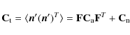
We write the time-ordered data (TOD) stream as

Here the first term presents the CMB signal and the second term presents noise. Vector
Since we are including polarization, map ![]() is an object of
is an object of
![]() elements, where
elements, where
![]() is the number of sky pixels.
In each pixel, the map consists of three values, corresponding to the three
Stokes parameters I, Q, U. The observed signal can be written as
is the number of sky pixels.
In each pixel, the map consists of three values, corresponding to the three
Stokes parameters I, Q, U. The observed signal can be written as
Here
We divide the noise contribution into a correlated noise component
and white noise, and model the correlated part as a sequence of uniform baselines,
Vector
Assuming that the white noise
component and the correlated noise component are independent,
the total noise covariance in time domain is given by
where
Maximum likelihood analysis yields the chi-square
minimization function
We want to minimize (5) with respect to both
Substituting Eq. (6) back into Eq. (5) and minimizing with respect to
where
A similar analysis without the noise covariance term
In some situations it is beneficial to solve the baselines at a resolution different from the resolution of the final map. Particularly, a strong signal error caused by a strong foreground signal can be reduced by destriping at a high resolution. Signal error is discussed in Sect. 6. We now extend our analysis to a case where the two resolutions are different.
Matrix
P depends on resolution. We define two different pointing
matrices: matrix
![]() is constructed at the destriping resolution
and matrix
is constructed at the destriping resolution
and matrix
![]() at the map resolution.
at the map resolution.
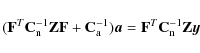
We estimate the baseline amplitudes by solving vector ![]() from Eq. (7),
where now
from Eq. (7),
where now
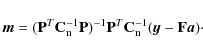
The final map is then constructed by binning the cleaned TOD into a map at a different resolution as
Strictly speaking, separating the two pointing matrices breaks the maximum likelihood analysis presented above, in the sense that the map constructed through Eqs. (7), (9), and (10) is not the solution of any maximum likelihood problem. In practice, the division works well and is intuitive.
We define two other maps, which are useful for further analysis,
and are products of the MADAM code.
The binned map is constructed without baseline extraction as
and is useful in signal-only simulations. The sum map

|
(12) |
is useful in the case of incomplete sky coverage, since it is well-defined also in pixels with poor sampling of polarization directions.
3 Noise prior
We consider now the statistical properties of the correlated noise component,
assumed to be stationary, and derive a formula for the noise prior
![]() .
In the first paper (Keihänen et al. 2005) we presented a method for the computation
of the noise prior for a general baseline function.
In the case of uniform baselines, the covariance can be constructed by a simpler
method as follows.
.
In the first paper (Keihänen et al. 2005) we presented a method for the computation
of the noise prior for a general baseline function.
In the case of uniform baselines, the covariance can be constructed by a simpler
method as follows.
Let c(t) denote the auto-covariance function of the time-ordered noise stream.
That is, the expectation value of the product of two samples of the noise stream,
time t apart, is given by
| (13) |
The auto-covariance may be expressed as a Fourier transform of the noise spectrum as
|
(14) |
This sets the normalization convention applied in this paper.
We assume that the spectrum P(f) is known.
We study now the covariance between two baselines of length T.
We define the reference value for a baseline offset, extending from time t to time t+T,
as an average of the noise stream,
|
(15) |
We calculate the noise prior
Consider a sequence of baselines, starting at times
![]() The correlation between the two baselines only depends on their distance.
We denote by
The correlation between the two baselines only depends on their distance.
We denote by
![]() any of the elements of
any of the elements of
![]() on the k:th diagonal.
We may write
on the k:th diagonal.
We may write
| (16) |
We need the inverse of matrix
|
(17) |
We now want to find a relation between
|
(18) |
which can be written in terms of the auto-covariance function c(t) as
|
(19) |
We further express this in terms of the noise spectrum,
|
(20) |
The integrals over t and t' can be carried out analytically, yielding
|
(21) |
We can now write out the baseline spectrum as
The sum over kyields zero unless f-f' is a multiple of 1/T, in which case it gives infinity. We may write, in terms of the delta function,
![\begin{displaymath}\sum_{k=-\infty}^{\infty}
{\rm e}^{{\rm i}2\pi k(f'-f)T} = \frac1T\sum_m[\delta(f'-f-m/T)].
\end{displaymath}](/articles/aa/full_html/2010/02/aa12813-09/img45.png)
|
(23) |
Substituting this into (22) gives
|
(24) |
To put this into a slightly more elegant form we use the formula
|
(25) |
The spectrum of the reference baselines can now be written in the final form as
If the noise spectrum decreases steeply with frequency, as is the case with 1/f noise, it is enough to evaluate only a few terms around m=0.
Once the spectrum (26) is known, it is straightforward to
compute the term
![]() ,
needed in the evaluation of Eq. (7), for an arbitrary baseline vector
,
needed in the evaluation of Eq. (7), for an arbitrary baseline vector ![]() ,
using the
Fourier technique.
,
using the
Fourier technique.
4 Implementation
![\begin{figure}
\par\includegraphics[width=9cm,clip]{1281302.eps}
\end{figure}](/articles/aa/full_html/2010/02/aa12813-09/img51.png)
|
Figure 2: Recovered 1/f noise. We show a one minute excerpt of simulated 1/f noise ( green), fitted with 0.625 s baselines (48 samples). The blue curve shows the reference baselines. The gray curve shows the combined 1/f + white noise timeline, averaged over the baseline period. The red curve above shows the baselines recovered by MADAM. There is an offset between recovered and actual noise, due to the fact that destriping cannot determine the mean of the noise stream. To help the comparison, we show by red dashed line the recovered noise stream lowered by 1 mK. |
| Open with DEXTER | |
MADAM is written in Fortran-90 and parallelized by MPI.
The code takes as an input the time-ordered data stream (TOD) for one
or several detectors, and pointing information, which consists of
three pointing angles
![]() for each TOD sample. Angles
for each TOD sample. Angles ![]() and
and ![]() define a point on the celestial sphere, while
define a point on the celestial sphere, while ![]() defines the orientation of the polarization sensitivity. Alternatively,
MADAM may construct the pointing angles from satellite pointing
data, using the known focal plane geometry.
defines the orientation of the polarization sensitivity. Alternatively,
MADAM may construct the pointing angles from satellite pointing
data, using the known focal plane geometry.
The noise prior is constructed from a noise spectrum given as input. MADAM does not make noise estimation herself. If the noise spectrum is unknown, the user may optionally turn off the noise prior, in which case MADAM becomes a traditional destriper.
As output, the code produces full-sky maps of intensity and Q and U polarization.
As additional information, the code may be set to output matrix
(
![]() ),
a hit count map, a sum map and a binned map,
and in case of incomplete sky coverage, a sky mask.
The code can also store the solved baseline offsets.
),
a hit count map, a sum map and a binned map,
and in case of incomplete sky coverage, a sky mask.
The code can also store the solved baseline offsets.
4.1 Solving the baselines
Matrices F and P, appearing in the destriping Eq. (7), are very large, but sparse. MADAM solves the baseline offsets from Eq. (7) by the conjugate gradient technique (CG), which is a standard technique for solving sparse linear systems, (see, for instance, Press et al. 1992). MADAM stores only the non-zero elements of the sparse matrices, and performs the matrix manipulations algorithmically.
The required number of iteration steps typically varies in the range of 15-100, depending on the baseline length and other input parameters. Once the baselines are solved, the final map is constructed by a binning operation defined by Eq. (10). We refer to these computation phases as the destriping phase and the binning phase.
We show in Fig. 2 a one-minute excerpt of simulated 1/f noise, together with the corresponding component recovered by MADAM. The recovered stream consists of baseline amplitudes solved by the code. We show also the reference baselines, obtained by averaging the 1/f noise over 0.625 s periods. The reference baselines can be regarded as the goal of baseline determination.
There is a global offset between the recovered and actual 1/f noise. This is due to the fact that destriping cannot distinguish between a global offset in the observed signal due to 1/f noise and a similar offset due to a CMB monopole. In conventional destriping (Keihänen et al. 2004; Burigana et al. 1997; Delabrouille 1998; Kurki-Suonio et al. 2009; Maino et al. 2002,1999) this manifests as a zero eigenvalue of the linear system to be solved. When a noise prior is present, the linear system is mathematically well-conditioned, and all eigenvalues are positive, as the prior forces the baseline average to zero. The actual noise average, however, remains undetermined, as in conventional destriping.
The sequence of solved baselines does not exactly follow that of reference baselines, even if the global offset is subtracted. This is due to the white noise component in the TOD, which causes uncertainty in the determination of the baseline amplitudes. The combined 1/f + white noise curve, binned over the baseline length, is shown Fig. 2 along with the recovered and reference baselines.
4.2 Pixelization
The division into the destriping and binning phases is a characteristic of the destriping technique. It opens interesting possibilities for handling signal error, or gaps in the TOD. By signal error we mean the error due to temperature variations within a sky pixel.
Destriping and binning may be carried out at different resolutions.
MADAM makes use of the HEALPix pixelization![]() ,
where the sky is divided into
,
where the sky is divided into
![]() equal-area pixels. The baseline amplitudes are first solved
at a destriping resolution, defined by parameter nside_cross.
The solved baselines are then subtracted from the TOD,
and the cleaned TOD is binned into a map at a map resolution,
defined by parameter
equal-area pixels. The baseline amplitudes are first solved
at a destriping resolution, defined by parameter nside_cross.
The solved baselines are then subtracted from the TOD,
and the cleaned TOD is binned into a map at a map resolution,
defined by parameter
![]() ,
which may be smaller or larger than nside_cross.
We study the effect of varying nside_cross in Sect. 8.
,
which may be smaller or larger than nside_cross.
We study the effect of varying nside_cross in Sect. 8.
MADAM allows to exclude a part of the sky, for instance the galaxy, defined by an input mask, in the destriping phase, while including all pixels in the final map. This feature may be used to reduce the effect of signal error, which for a large part comes from the foreground-dominated parts of the sky. Signal error is discussed in Sect. 6.
In our first paper (Keihänen et al. 2005) we considered only temperature measurements. In that case it was possible to determine a temperature value for every sky pixel that is hit by any detector at least once. An additional complication arises when polarization is involved. To accurately determine the three Stokes parameters for all pixels, a sufficient coverage in polarization angle is needed in every pixel. If that is not the case, the Stokes parameters in a pixel become degenerate. This may happen for instance, if a pixel is visited by only one P LANCK detector pair. Such pixels may still be used for determination of the baseline offsets. MADAM does this by dropping the (nearly) zero eigenvalues and the corresponding eigenvectors from the pixel matrix in the destriping phase. In the binning phase the degenerate pixels must be excluded entirely.
4.3 Gaps
![\begin{figure}
\par\includegraphics[width=9cm,clip]{1281303.eps}
\end{figure}](/articles/aa/full_html/2010/02/aa12813-09/img58.png)
|
Figure 3: Effect of gaps. We fit 0.625 s (48 samples) baselines to a region where part of the data is missing. We indicate the gaps by shading. There is one wider gap (10 s), centered around t=30 s, and 16 narrow ones (12 samples). The thick blue curve shows the sequence of recovered baselines in the case all data is there. The red curve shows the recovered baselines when the gaps are inserted. For comparison we show ( purple interrupted curve) a case where the data is appended end-to-end and treated as continuous. |
| Open with DEXTER | |
The division of noise into a white noise component and a correlated noise component offers a natural way of handling gaps in TOD. By a gap we mean a sequence of samples which are missing from the continuous TOD stream. The data may be corrupted and useless for analysis, or missing entirely. If the data sections on both sides of the gap are appended end-to-end, or filled, gaps destroy the assumption of noise stationarity, which leads to boundary effects around the gap. A more clever way to handle gaps is to flag the corrupted samples, and to set the variance of the white noise component to infinity for the flagged samples. Remember that we assumed that the correlated noise component is stationary, but we did not make the same assumption for the white noise component. In practice this done by pointing the flagged samples into a dummy pixel, which is excluded in matrix operations which involve picking a TOD from a map. The flagged samples are effectively excluded from map-making, while the correct statistical properties of the correlated noise component are still preserved across the gap.
Two fundamentally different cases may be distinguished. If a gap is longer than the chosen baseline length, some baselines fall completely inside it. MADAM determines a constrained realization of amplitudes also for these baselines, with the help of the noise prior and the available data on both sides of the gap. The baselines inside the gap do not contribute directly to the final map, but they have an effect on the baselines solved on both sides of the gap. If no noise prior is used, baseline amplitudes become zero inside the gap.
If a gap is shorter than the baseline, some samples on the baseline are missing, but the baseline amplitude may still be determined based on the remaining samples, of course with less accuracy.
We demonstrate this in Figs. 3 and 4. We have inserted one ``large'' (10 s) gap and 16 small (12 samples, or 0.15 s) gaps. We show the sequence of baselines in the case all data is there, and in the case of gaps.
In Fig. 3 we show a one minute chunk of solved 0.625 s baselines, with all the data present, or with gaps inserted. This is the same data chunk as in Fig. 2. For comparison we also show what happens if the data is appended end-to-end over the gap. In the latter case, the discontinuity in data leads to a strong boundary effect, which destroys the fit on both sides of the gap. No such boundary effect is present when the gap is handled as explained above.
In Fig. 4 we show a blow-up of the region where we have inserted gaps shorter than the baseline. The effect is less dramatic there.
![\begin{figure}
\par\includegraphics[width=9cm,clip]{1281304.eps}
\end{figure}](/articles/aa/full_html/2010/02/aa12813-09/img59.png)
|
Figure 4: Blow-up of the 3-12 s region of Fig. 3. |
| Open with DEXTER | |
4.4 Split-mode
Map-making with a short baseline requires a large run-time memory. One way of reducing the memory requirement is the split-mode. Data is split into small sections, each of which is destriped independently. Destriping in small pieces tends to leave the lowest frequency component of each piece poorly determined, which shows as relative offsets in different parts of the sky, when the data sections are combined into one map. We therefore re-destripe the already cleaned TOD, this time simultaneously, but with a long baseline (typically 1 h). The total memory requirement in split-mode can be pushed significantly lower than in standard mode, at the cost of increased CPU time requirement. Also the map quality suffers slightly as compared to the standard mode.
4.5 Computational resources
The memory requirement of the code is in most cases dominated by
the storage of pointing information. Our simulation data set contains 16 months of data for
4 detectors, at a sampling frequency of 76.8 Hz.
The pointing information for each sample consists of a pixel number
(4 bytes) and factors
![]() and
and
![]() (4 bytes
each). The pointing information for the whole 488-day data set takes
(4 bytes
each). The pointing information for the whole 488-day data set takes
![]() bytes, 145 gigabytes alltogether.
bytes, 145 gigabytes alltogether.
TOD is read into a buffer a small piece at a time, and binned to form the right-hand-side of the destriping equation. Pointing data instead, must all be kept in memory simultaneously.
When the baseline length exceeds the scanning period, several samples on one baseline may fall on the same pixel. In such a situation MADAM combines the samples to reduce the memory requirement. The compression is lossless, i.e. the compression has no effect on the output map, just on the resource requirement. Compression reduces the memory requirement significantly when using long baselines.
Table 1: Computational resources for various combinations of input parameters.
All our simulations were run on the Cray XT4/XT5 ``Louhi'' system of CSC (IT Center for Science), Finland. We used from 32 to 128 processors. The number of processors was selected according to the memory requirement.
In Table 1 we list the computational resources for various runs. In all the listed cases, we built intensity and polarization maps of the full data set (488 days, 4 detectors at sampling frequency of 76.8 Hz). We vary the baseline length and destriping resolution. In the first column we show the parameter we have varied, that is the baseline length, resolution in the destriping phase, or the number of data chunks in split-mode. The other columns show the number of conjugate-gradient iteration steps, total memory usage, number of processors, and CPU time usage as wall-clock time and as CPU hours.
The memory requirement depends strongly on the chosen baseline length at long baselines (above 60 s) because the effectiveness of data compression strongly depends on how many samples on a baseline fall on the same pixel.
The split-mode offers a trade-off between memory and CPU time usage. When data is destriped in small chunks, memory usage can be pushed very low, but at the same time the required CPU time increases drastically.
5 Simulations
We created a set of simulated time-ordered data, mimicking the data from the Planck LFI (Low-Frequency Instrument) 70 GHz channel. The TOD was produced using P LANCK LevelS simulation software (Reinecke et al. 2006). We created data for 16 months for four detectors, corresponding to the LFI horns 19 and 22.
We ran MADAM on this simulation data with different parameter settings. Results are discussed in the following sections.
For each of the four detectors, we created four TOD streams of 16 months duration:
a CMB signal, a foreground signal, 1/f noise, and white noise.
Each TOD consisted of
![]() samples.
Storing the TOD components separately allowed us to do noise-only and signal-only
simulations.
samples.
Storing the TOD components separately allowed us to do noise-only and signal-only
simulations.
Pointing information was stored in the form of satellite pointing, sampled at 1 s intervals. MADAM constructed detector pointings, sampled at the sampling frequency 76.8 Hz, with the help of focal plane parameters.
The same data set was used by Kurki-Suonio et al. (2009), with the exception that in this work we used 16 months of data (instead of 12). We have also included a foreground component.
5.1 Scanning
The scanning strategy imitates that of the actual P LANCK spacecraft (Dupac & Tauber 2005).
The spin axis rotated around
the anti-Sun direction once every six months, in a circle of radius
![]() .
When projected onto the sky, this creates a cycloidal path.
The spin axis was repointed at fixed intervals of one hour. Between
repointings, the spin axis nutated with a mean amplitude
.
When projected onto the sky, this creates a cycloidal path.
The spin axis was repointed at fixed intervals of one hour. Between
repointings, the spin axis nutated with a mean amplitude
![]() .
.
The detectors scanned the sky almost along great circles. The
satellite rotated around the spin axis with a mean rate of
![]() Hz (one rotation per minute). The detectors were
pointed
Hz (one rotation per minute). The detectors were
pointed
![]() away from the spin axis.
Small variations (rms 0.1
away from the spin axis.
Small variations (rms 0.1
![]() /s) were added to the spin rate.
Because of the nutation and the spin rate variations, adjacent
scanning circles did not fall exactly on top of each other.
/s) were added to the spin rate.
Because of the nutation and the spin rate variations, adjacent
scanning circles did not fall exactly on top of each other.
The two detectors belonging to the same horn shared the same
pointing (
![]() )
on the sky, but the polarization angles
were different by 90.0
)
on the sky, but the polarization angles
were different by 90.0
![]() .
The two horns followed the same path,
but one horn trailed the other by 3.1
.
The two horns followed the same path,
but one horn trailed the other by 3.1
![]() .
The polarization
angles of the two horns were roughly at 45
.
The polarization
angles of the two horns were roughly at 45
![]() angles, so that
the polarization measurements of the two horns complemented each
other. For a more detailed description of the scanning strategy see
Kurki-Suonio et al. (2009).
angles, so that
the polarization measurements of the two horns complemented each
other. For a more detailed description of the scanning strategy see
Kurki-Suonio et al. (2009).
During the 16 month observation time the four detectors covered each pixel on the sky at resolution nside_map = 512 in multiple polarization directions. Therefore we were able to determine the three Stokes components in every pixel.
5.2 Signal
Our simulation data set contained signal from CMB and from
foregrounds.
No dipole signal was included.
We used the CAMB![]() code to
produce a theoretical CMB angular power spectrum with cosmological
parameter values
code to
produce a theoretical CMB angular power spectrum with cosmological
parameter values
![]() .
We then created a realization of
coefficients
.
We then created a realization of
coefficients
![]() and
and
![]() .
No B mode polarization was
included. We constructed a TOD with sampling frequency
.
No B mode polarization was
included. We constructed a TOD with sampling frequency
![]() Hz, smoothing with a symmetric Gaussian beam with
FWHM =
Hz, smoothing with a symmetric Gaussian beam with
FWHM =
![]() (Wandelt & Górski 2001; Challinor et al. 2000).
(Wandelt & Górski 2001; Challinor et al. 2000).
The foreground signal included Galactic emission from thermal and
spinning dust, synchrotron radiation, and free-free scattering. On
top of the galactic signal we added a Sunyaev-Zeldovich signal, and
weak point sources. We constructed an
![]() sky map including
these components, using the Planck sky model, PSM, version 1.6.3
sky map including
these components, using the Planck sky model, PSM, version 1.6.3![]() .
The map was smoothed with a symmetric gaussian beam.
We then constructed the foreground TOD
by picking values from the input map according to the scanning
pattern.
.
The map was smoothed with a symmetric gaussian beam.
We then constructed the foreground TOD
by picking values from the input map according to the scanning
pattern.
5.3 Noise
We generated 1/f noise by the SDE (Stochastic Differential equation) algorithm,
which builds the noise stream as a linear combination of a number
of low-pass filtered white noise streams
(Reinecke et al. 2006).
We used the following input parameters:
knee frequency of
![]() Hz, sampling frequency
Hz, sampling frequency
![]() Hz, slope
Hz, slope
![]() ,
and minimum frequency
,
and minimum frequency
![]() Hz.
On top of the 1/f noise we added Gaussian white noise with a standard deviation of
Hz.
On top of the 1/f noise we added Gaussian white noise with a standard deviation of
![]() mK and zero mean.
mK and zero mean.
We have chosen a high knee frequency in order to show clearly the effect of correlated noise in the output maps. The purpose of these simulations is not to demonstrate the actual performance of the P LANCK experiment, but to give a quantitative picture of how changing the various parameters which control the MADAM algorithm affects the quality of output map and the required computational resources.
We show the noise spectrum in Fig. 5 together with
the analytical model used to construct the noise prior. We computed
the noise spectrum through the Fourier technique from noise streams
of 366 h, averaging over 32 independent noise realizations, at
100 distinct frequencies. The analytical model describes the noise
well at high frequencies, but differs somewhat at low frequencies.
The analytical model is given by
| P(f) | = | 
|
(27) |
| P(f) | = | 
|
It is possible to theoretically predict the spectrum produced by the SDE algorithm. The prediction is plotted in the same figure, and agrees well with the actual spectrum.
![\begin{figure}
\par\includegraphics[width=9cm,clip]{1281305.eps}
\end{figure}](/articles/aa/full_html/2010/02/aa12813-09/img81.png)
|
Figure 5: Noise spectrum. The dashed red line shows the analytical 1/f noise model used when constructing the noise prior. The solid blue line gives the actual spectrum of the input noise, computed as an average over 32 noise realizations. The dash-dotted purple line presents the numerically predicted SDE spectrum. We show also the white noise spectrum ( dashed blue) and the sum of the white and 1/f noise ( solid black). |
| Open with DEXTER | |
![\begin{figure}
\par\includegraphics[angle=90,width=8.5cm,clip]{1281306a.ps} \inc...
...81306b.ps} \includegraphics[angle=90,width=8.5cm,clip]{1281306c.ps}
\end{figure}](/articles/aa/full_html/2010/02/aa12813-09/img82.png)
|
Figure 6: Full-sky maps. From top to bottom: binned noiseless map (total intensity), map directly binned from TOD, and destriped map (baseline length 0.625 s). The binned map is contaminated by stripes due to 1/f noise. |
| Open with DEXTER | |
6 Residual error
![\begin{figure}
\par\includegraphics[angle=90,width=8.5cm,clip]{1281307a.ps} \includegraphics[angle=90,width=8.5cm,clip]{1281307b.ps}
\end{figure}](/articles/aa/full_html/2010/02/aa12813-09/img83.png)
|
Figure 7: Residual noise. Upper map shows the residual noise map. The bottom map shows the correlated residual, which we obtain by subtracting the binned white noise from the residual noise map. Note the difference in scale. |
| Open with DEXTER | |
To assess the quality of the destriped map, we study first the residual error map, which we compute as the difference between the destriped map and the binned noiseless map. The binned noiseless map is obtained by binning the simulated signal TOD into a map as by Eq. (11).
The top panel of Fig. 6 shows the binned noiseless map. We show also the map binned from noise-contaminated TOD, and the destriped map. The map binned from noisy data is contaminated by stripes due to 1/f noise. The difference between the bottom and top panels is the residual error map.
The residual error map can further be divided into two statistically independent components: the signal error map and the residual noise map. The signal error map is obtained by destriping the signal-only TOD and subtracting the binned noiseless map from it. The residual noise map is obtained by destriping the noise-only TOD. Because destriping is a linear process, the total residual error is a sum of signal error and residual noise.
Signal error arises from temperature variations within a pixel, which the code interprets as noise and which lead to non-vanishing baseline amplitude estimates even in absence of noise. The signal error has the undesired effect of spreading sharp features in the signal map along the direction of the scanning ring.
Residual noise is strongly dominated by white noise. Though it is the dominant component, it is rather simple to handle at later data processing levels, for instance power spectrum estimation. We are more interested how much correlated noise there is left in our output maps. We therefore subtract the binned white noise map from the residual noise map, and study the remaining correlated residual noise (CRN) map separately.
The residual noise map, as well as its correlated component, are depicted in Fig. 7.
It can be shown that the CRN map and the binned white noise map are statistically independent, if the final map is binned to a resolution equal to or lower than the destriping resolution. The proof was presented by Kurki-Suonio et al. (2009) for the case of equal resolutions. Here we show that the maps are independent also if the destriping resolution is higher than the map resolution.
The binned white noise map is proportional to the quantity

|
(28) |
where
|
(29) |
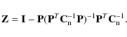
The correlation between the two maps is proportional to

|
(30) |
From the definition of Z one sees that
If the map is binned to a resolution higher than the
destriping resolution, we have the opposite relation
![]() .
In that case, the correlation between the CRN
map and the binned white noise map does not vanish. This has some
interesting consequences, which are discussed in Sect. 8.
.
In that case, the correlation between the CRN
map and the binned white noise map does not vanish. This has some
interesting consequences, which are discussed in Sect. 8.
Residual noise does not share the symmetry of the original noise. Residual noise is not stationary in the time domain, like the original 1/f noise. Note also that no noise component is statistically isotropic in the map domain. A complete description of the residual noise requires the calculation of the noise covariance matrix (NCVM), which is outside the scope of this paper. Computation of the NCVM for low-resolution maps is discussed by Keskitalo et al. (2009).
In this paper we calculate some simple figures of merit, which describe different aspects of the residual noise. In cases where the binned white noise map and the CRN map are independent, the variance of the CRN map is a useful number. It has the benefit of describing the residual noise level as one number, which can be plotted as a function of various parameters. We calculate the variance of the CRN map for the three Stokes maps, I, Q, U, separately.
Variance is an additive number. When the residual error map can be divided into independent components, we compute and plot the variance of each individual component separately. The total variance of the residual error is obtained as the sum of variances of the individual components.
When destriping is performed at a resolution lower than the map resolution, the CRN map and binned white noise are correlated. In this situation also the covariance between the two maps is an important quantity. The covariance is expressed in the same units as the variance, which makes it easy to compare the two. This is the main reason why we have chosen to use the variance as the main figure of merit, instead of rms. The covariance is computed by averaging over all sky pixels the product of temperature values of the two maps in question.
We calculate also the spectrum of the residual noise in time domain, as a square of the Fourier transform of the noise stream. Neither this is a complete description of the residual noise, because the residual noise is not stationary (not diagonal in Fourier domain).
Finally, we calculate the angular power spectrum of the residual noise map. Again, because the residual noise is not statistically isotropic, the angular power spectrum does not fully describe the noise, but gives an idea at which scales the noise is distributed in the map domain. It also gives the noise bias which should be subtracted from the spectrum of the destriped map to get an unbiased estimate of the power spectrum of the underlying signal map.
In Fig. 8 we show first the spectrum of the CRN map for 0.625 s baseline length, together with the spectrum of the binned noiseless map. We show also the white noise level.
7 Effect of baseline length
7.1 Map domain
In this section we study the effect of baseline length on the residual
noise. We destripe and bin the final map at a fixed resolution
nside_cross = nside_map = 512. The destriped map consists of 3 million
pixels (
![]() )
for each of the three Stokes
components.
)
for each of the three Stokes
components.
Since we destripe and bin the map at the same resolution, the binned white noise map and the correlated residual noise (CRN) map are statistically independent.
![\begin{figure}
\par\includegraphics[width=9cm,clip]{1281308a.eps}\par\includegraphics[width=9cm,clip]{1281308b.eps}
\end{figure}](/articles/aa/full_html/2010/02/aa12813-09/img93.png)
|
Figure 8: Angular power spectrum of signal and residual noise. We show TT and EE spectra of the correlated residual noise (CRN) map ( blue curve), together with the spectra of the binned noiseless CMB map black. Also shown is the white noise level ( purple dashed line). The baseline length was 0.625 s. |
| Open with DEXTER | |
![\begin{figure}
\par\includegraphics[width=9cm,clip]{1281309.eps}
\end{figure}](/articles/aa/full_html/2010/02/aa12813-09/img94.png)
|
Figure 9: Effect of baseline length on residual error. The residual error map is divided into three components: binned white noise (above), correlated residual noise ( middle), and signal error (below). We show the variance of each residual component map, as a function of baseline length. Binned white noise is independent of baseline length, and its variance is shown by a straight line. We show the three Stokes parameters I, Q, U ( blue solid, purple dashed, and red dash-dotted line, respectively). The dotted lines show the effect of turning the noise prior off. At long baselines results with and without noise prior coincide. |
| Open with DEXTER | |
In Fig. 9 we plot the variance of various components of the residual error map, as a function of baseline length. We show the variance of the signal error map, CRN map, and binned white noise map, for the three Stokes parameters (I, Q, U). We show results both with and without noise prior. The total variance is the sum of the three components.
We discuss in the following the dependence of the results on baseline length. Some features are readily visible.
The variance of the binned white noise is, obviously, independent of baseline length.
As a general trend, correlated residual noise decreases with decreasing baseline length, as the noise becomes better modelled by the selected baselines. Baseline lengths which are an integer fraction of the repointing period (1 h), give a local minimum. Below 1 s the results converge. In the remainder of this paper we often use baseline length 0.625 s (48 samples) as an example of a very short baseline. At this baseline length, results have already converged with respect to baseline length, but requirements for computational resources are still moderate.
As opposite to residual noise, signal error increases with decreasing baseline length, but remains always below the noise level. Signal error becomes more important if destriping is performed at a low resolution. We discuss this in Sect. 8.
The noise prior has a negligible effect on results above 1 min (![]()
![]() )
baseline length. At short baselines (<
)
baseline length. At short baselines (<
![]() ),
on the contrary, the noise prior becomes important. When the noise
prior is turned off, the required CPU time increases steeply with
decreasing baseline length, as the algorithm requires a large number
of iteration steps to converge. Therefore we have not computed
results without the noise prior at the very shortest baseline
lengths.
),
on the contrary, the noise prior becomes important. When the noise
prior is turned off, the required CPU time increases steeply with
decreasing baseline length, as the algorithm requires a large number
of iteration steps to converge. Therefore we have not computed
results without the noise prior at the very shortest baseline
lengths.
The variance of residual noise for Q and U is above that of I, roughly by a factor of 2. This reflects the fact that Q and U contribute to the observed signal weighted by factors
![]() ,
,
![]() (Eq. (2)) relative to I.
(Eq. (2)) relative to I.
The signal error in Q and U is well below that of the temperature component. This follows directly from the fact that the polarization signal is weaker than the intensity signal.
To show the behaviour of the CRN curve more clearly, we plot it separately for long and short baselines in Figs. 10 and 11.
Baseline lengths which are an integer fraction of the repointing period (here 1 h), give a clear and sharp local minimum. The minimum is deepest at 1 h baseline length, but strong dips can also be seen at baseline lengths 30 min, 20 min, 15 min, 12 min and 10 min.
The dip structure is obviously related to the scanning strategy. Why the use of baselines that fit into destriping periods is better than the use of ones that do not, can be understood when thinking of an ideal scanning, where scanning rings fall exactly on top of each other. The noise stream can be thought as composed of two components: an ``offset'' component consisting of 1 min reference baselines, defined as averages of the noise stream over 1 min periods, and a second component which contains the remaining high-frequency noise. The offset component dominates the noise. When the noise stream is averaged over 60 adjacent scanning circles, the offset component produces a residual offset, equal to the average of 60 adjacent reference baselines. When the data is destriped with a one-hour baseline, destriping effectively removes the residual offset. If the baseline length differs from one hour, a time offset develops between baselines and repointing periods, with the result that noise offsets do not cancel out.
In this work we have assumed a scanning strategy, where the repointing period is constant at 1 h, as was originally planned for Planck, and study only constant baseline lengths. In reality, Planck is likely to use a scanning pattern where the repointing period varies. We have not run simulations with a variable pointing period, but based on the results presented here, we expect that for optimal results the baseline length should follow the repointing period, if a long baseline length is required. A varying baseline length has therefore been implemented in MADAM for the use of the P LANCK experiment.
![\begin{figure}
\par\includegraphics[width=9cm,clip]{1281310.eps}
\end{figure}](/articles/aa/full_html/2010/02/aa12813-09/img97.png)
|
Figure 10: Long baselines. Variance of the CRN map as a function of baseline length, for long baselines. This is a blow-up of the long-baseline part of the CRN curves in Fig. 9. We have computed the residual noise at 1 min intervals. Baseline lengths that go evenly into the repointing period of 1 h, stand out as local minima. |
| Open with DEXTER | |
![\begin{figure}
\par\includegraphics[width=9cm,clip]{1281311.eps}
\end{figure}](/articles/aa/full_html/2010/02/aa12813-09/img98.png)
|
Figure 11: Short baselines. We show the CRN variance as a function of baseline legth, for short baselines. This is a blow-up of the short-baseline part of the CRN curves in Fig. 9. We show again the three Stokes parameters with different line types. The upper, thin lines show the effect of turning off the noise filter. |
| Open with DEXTER | |
![\begin{figure}
\par\includegraphics[width=9cm,clip]{1281312.eps}
\end{figure}](/articles/aa/full_html/2010/02/aa12813-09/img99.png)
|
Figure 12: Ideal noise. We show the CRN variance as a function of baseline length for real noise (same as in Fig. 9) and for idealized noise, composed of reference baselines. |
| Open with DEXTER | |
When no noise prior is used, the CRN variance as a function of baseline length has a global minimum, as a result of two competing effects. When moving towards shorter baselines, noise becomes better modelled. On the other hand, the shorter the baselines, the more there are unknowns (baseline amplitudes) to be solved, while the amount of data remains fixed. With our data set the optimal baseline length was 10 s. Kurki-Suonio et al. (2009) split the CRN map further into residual 1/f noise and white noise baselines to study these competing effects more deeply. The optimal baseline length depends on the knee frequency of the 1/f component.
With the noise prior, results continue to improve at least until baseline lengths of 0.1 s, which is the limit where we could bring our computations. The noise prior has the effect of restricting the baseline solution in such a way that the effective number of unknows does not follow the number of baselines.
In order to study the importance of the high-frequency part of the noise spectrum, which is not well modelled by baselines, we made a simulation where we removed the part of noise not modelled by the baseline approximation. For each baseline length, we replaced the 1/f noise component by a sequence of baselines of the same length as the baseline length used in destriping. The results are shown in Fig. 12, together with results obtained with realistic noise. The difference between the two sets of curves is the contribution of noise not modelled by baselines. We see that this component becomes very important at long baselines.
![\begin{figure}
\par\includegraphics[width=9cm,clip]{1281313.eps}
\end{figure}](/articles/aa/full_html/2010/02/aa12813-09/img100.png)
|
Figure 13:
Split-mode. Residual correlated noise variance for
split-mode, as a function of the splitting factor. In the first
phase data was destriped in chunks of length 488 days/
|
| Open with DEXTER | |
In Fig. 13 we show results obtained by applying the split-mode. Data was divided into chunks which were first destriped separately with a 0.625 s baseline. In the second phase we combined the chunks, and re-destriped the data with 1-h baselines. The rightmost points correspond to a case where the data was destriped in 1-day chunks. The leftmost point corresponds to the standard case, where the whole 488-day data set is destriped once. The CRN variance in split-mode is higher than in the standard mode. This reflects the fact that the split-mode does not exploit all information in the data. The benefit of the split-mode is that it requires less memory than the standard mode, as can be seen from Table 1.
7.2 Time domain
![\begin{figure}
\par\includegraphics[width=9cm,clip]{1281314.eps}
\end{figure}](/articles/aa/full_html/2010/02/aa12813-09/img101.png)
|
Figure 14: Effect of baseline length on residual noise spectrum. We subtract the solved baselines from the noise TOD (white noise and 1/f noise) and plot the spectrum of the residual. We show results for 7 baseline lengths, from above: 1 h ( black), 15 min ( yellow, 4 min ( purple), 1 min ( cyan), 15 s ( red), 2.5 s ( green) and 0.625 s ( blue). Solid and dashed lines show results with and without noise prior, respectively. With 1 min baselines and longer, the dashed and solid curves (noise prior on/off) are on top of each other. The 0.625 s case with noise prior, which of the studied cases gives the lowest residual noise variance in map domain, is shown by a thick linetype. Also shown are the original noise spectrum ( black dashed) and the analytical approximation given by Eq. (31) ( black dash-dotted). |
| Open with DEXTER | |
Next we consider the residual noise in the TOD domain. We subtract the solved baselines from the combined white noise plus 1/f noise TOD, and compute the spectrum of the residual. We plot the spectrum for various baseline lengths in Fig. 14. We show results both with and without noise prior. At long baselines (1 min and above) results with and without noise prior cannot be distinguished. When we move towards shorter baselines, differences appear. Without noise prior, residual noise power systematically decreases with decreasing baseline length. A peak structure appears at shortest baselines. When a noise prior is used, the spectrum of residual noise converges towards the spectrum shown by a thick line in the figure.
It is interesting to note that with a given baseline length, not applying a noise prior gives lower residual noise power in TOD domain. The situation becomes the opposite when the cleaned TOD is binned into map: using a noise prior leads to lower residual noise in map domain. This is related to the correlation properties of the destriped TOD. When a noise prior is applied, the residual TOD comes out less strongly correlated than without noise prior, and its spectrum closer to that of white noise. The TOD thus averages out more efficiently when binned into a map, leading to a lower noise level in map domain.
We plot in the same figure an analytical approximation
where
The behaviour of the residual noise spectrum in the absence of noise prior is discussed in detail by Kurki-Suonio et al. (2009).
7.3 Cl domain
Finally we study the residual noise in the Cl domain. We compute the TT and EE angular power spectra of the CRN map using the Anafast tool which is part of the HEALPix package.
In Fig. 15 we plot the spectrum of the CRN map for three distinct baseline lengths (1 h, 1 min, and 0.625 s) together with the spectrum of the binned noiseless map. Destriping resolution was nside_cross = 512. We show low and high multipoles separately. At high multipoles we bin the spectra over 16 adjacent multipoles, in order to show the differences more clearly. The TT plots begin at multipole l=1, the EE plots at l=2.
We show also the effect of a high destriping resolution (nside_cross = 2048). This case is discussed in more detail in Sect. 8. All spectra were computed from maps with resolution nside_map = 512.
We see that a short baseline (0.625 s) gives systematically lower residual noise than a longer one (1 min or 1 h) at all but the very lowest multipoles, though the difference is small as compared to the white noise level. In the EE spectrum the differences are comparable to the underlying CMB signal.
At the very lowest multipoles the situation is not that clear, but we remind here that we have one noise realization only, so the effects seen at lowest multipoles may be somewhat random.
8 Destriping resolution
![\begin{figure}
\par\hbox{
\includegraphics[width=9cm,clip]{1281315a.eps}\include...
...s}\includegraphics[width=9cm,clip]{1281315d.eps} }
\vspace*{9mm}
\end{figure}](/articles/aa/full_html/2010/02/aa12813-09/img105.png)
|
Figure 15: Noise bias. We show TT and EE spectra of the CRN (correlated residual noise) map. All spectra were computed from nside_map = 512 maps. We compare three baseline lengths: 0.625 s ( solid blue line), 60 s ( solid magenta line), and 3600 s ( dashed red line). Destriping resolution was nside_ cross = 512 for these three curves. We show also the effect of a high ( nside_ cross = 2048) destriping resolution ( green dashed line.) Also shown is the spectrum of the binned CMB map ( black solid line) and the white noise level ( black dashed line). The leftmost panels show the spectra at low multipoles in logarithmic scale. The rightmost panels show the spectra at high multipoles in linear scale. For clarity, the CRN spectra were averaged over 16 adjacent multipoles. |
| Open with DEXTER | |
![\begin{figure}
\par\includegraphics[width=9cm,clip]{1281316.eps}
\end{figure}](/articles/aa/full_html/2010/02/aa12813-09/img106.png)
|
Figure 16: Effect of destriping resolution on residual noise. We plot the residual noise variance against the base-2 logarithm of the nside_ cross parameter, for total intensity. We show the signal error ( red, open circles), CRN ( blue, solid circles), and covariance between CRN and white noise ( purple, squares). The black dashed line shows the sum of the CRN variance and twice the covariance between CRN and white noise. |
| Open with DEXTER | |
In this section we study how varying the destriping resolution affects the residual noise. We also study the effect of applying a galactic mask in the destriping phase.
We vary the destriping resolution nside_cross, which defines the crossing points, but bin the final map at a fixed resolution of nside_map = 512. We use baseline length 0.625 s and a noise prior. The effect of destriping resolution in traditional destriping was studied earlier by Maino et al. (2002).
In Fig. 16 we show the variance of different residual error components
as a function of destriping resolution.
We destriped the data with 7 distinct HEALPix resolutions:
(from left to right:
nside_cross = 32, 64, 128, 256, 512, 1024, 2048.)
Maps were binned to resolution nside_map = 512. We plot the residual
noise variance against the base-2 logarithm of the nside_cross
parameter, for total intensity. We show the
signal error, CRN, and covariance between CRN and white noise.
The total variance is the sum of these three
and the variance of white noise,
which is 2478 ![]() K2.
The signal error in the I map increases
rapidly with decreasing resolution, being 189
K2.
The signal error in the I map increases
rapidly with decreasing resolution, being 189 ![]() K2 at
nside_cross = 32.
Baseline length was 0.625 s.
K2 at
nside_cross = 32.
Baseline length was 0.625 s.
When the TOD is destriped at a resolution lower than the map resolution, the binned white noise map and the CRN map, which is obtained by subtracting the binned white noise map from the total residual noise, become correlated. For this reason, the variance of the CRN map alone is not a good figure-of merit. In addition to the CRN variance we compute the covariance between the CRN map and the binned white noise map, and plot the it together with the CRN variance.
We show in the same plot the sum of the CRN variance and twice the covariance between CRN and binned white noise. The total variance of the residual noise map is the obtained by adding the variance of the binned white noise map to this sum. The white noise level is a constant when nside_map is fixed.
At low resolutions the sum curve falls below zero. This indicates an interesting phenomenon. Destriping with a low resolution actually leads to a residual noise variance below the white noise level. This contradicts the often-heard claim that the white noise level sets a lower limit for the residual noise level that can be achieved by any map-making method. The drawback is of course that the residual noise is correlated.
The signal error depends on the resolution much more steeply than the residual noise. Larger pixels give rise to a larger signal error, as temperature variations within a pixel become more important. The signal error for the polarization maps is well below that of the intensity map, as we showed in Sect. 7. This reflects the fact that the polarization signal is weak compared to the total intensity.
The signal error is difficult to remove at later data processing steps, and hard to model reliably. It may cause undesired artifacts in the output map. For instance, signal error tends to spread the image of a strong point source into a line following the scanning pattern. It is desirable to minimize the signal error at the map-making level, by destriping at a sufficiently high resolution.
The signal error may be further reduced by masking out the pixels with highest temperature variation.
Differences in signal error above resolution nside_cross = 512 are hardly visible in Fig. 16. We study now the high resolution range (nside_cross = 512-2048) more closely.
We show our results for the high resolution regime in Table 2. We show the rms of the signal error and CRN maps, for total intensity and Q polarization. Here we have chosen to show the rms, instead of the variance, in order to have numbers comparable in magnitude. Maps were binned to a common resolution nside_map = 512. Baseline length was 0.625 s in all cases.
We show also the effect of applying a galactic mask in the destriping phase. We mask out 5% or 10% of the most strongly foreground-dominated pixels when solving the baseline offsets, but include them again when binning the cleaned TOD into the final map.
The reduction in signal error with increasing destriping resolution continues until our highest resolution nside_cross = 2048. in the same time, the residual noise increases slightly. Masking the galaxy reduces the signal error in the intensity map significantly. The difference between 5% and 10% masks is small. Because our simulation data set did not include polarized foregrounds, masking the galaxy has little effect on the signal error in the polarization map.
Table 2: Reducing signal error.
![\begin{figure}
\par\includegraphics[width=9cm,clip]{1281317.eps}
\end{figure}](/articles/aa/full_html/2010/02/aa12813-09/img108.png)
|
Figure 17: Effect of destriping resolution on the residual noise spectrum. We plot the spectrum of residual noise TOD, obtained by subtracting the solved baselines from the original noise TOD. The baselines were solved at resolution (from top down) nside = 2048 ( green), 512 ( blue) or 128 ( red). The black dashed line presents the analytical approximation given by Eq. (31). |
| Open with DEXTER | |
As in the previous section, where we studied the effect of baseline length, we study the noise residual also in the time domain and in the Cl domain. In Fig. 17 we plot the spectrum of the residual noise TOD for three destriping resolutions, nside_cross = 2048, 512, 128. Baseline length was again 0.625 s in all cases. We show also the analytical approximation given by Eq. (31).
A high destriping resolution clearly leaves more noise in the TOD at intermediate scales.
Going from resolution nside_cross = 512 to nside_cross = 128 has little effect on the spectrum above 1 mHz, but brings the spectrum down at lower frequencies. At the same time, the peaky structure in the spectrum becomes more pronounced.
Note that the spectrum of the residual noise TOD is only dependent on the destriping resolution nside_cross, and has nothing to do with the map resolution. Thus the dependence or independence of CNR and white noise in the map domain plays no role here.
Though the difference between nside_cross = 512 and nside_cross = 2048 shows clearly in the residual noise spectrum, the effect is less dramatic in the angular power spectrum of the CRN map. We compare the two cases in Fig. 15. The higher destriping resolution leaves slightly more noise at nearly all multipoles, but the effect is small compared with the effect of the baseline length.
9 Conclusions
We have presented an update of the MADAM map-making method and applied it to simulated Planck-like data. We produced maps of total intensity and Q and U polarization.
The MADAM algorithm is tuned by selecting values for a set of input parameters. We have studied the effect of baseline length and destriping resolution on residual error.
MADAM differs from traditional destripers in that it uses a noise prior, which allows to extend the method to very short baselines, which model the noise better. The noise prior has little effect on the results at baseline lengths longer than the inverse of the knee frequency, but becomes important at short baselines.
We varied the baseline length from 0.1 s to over one hour. We obtained best results when the baseline length was below one second. Our simulations assumed a knee frequency of 50 mHz.
For a Planck-like scanning strategy, long baselines, longer than the spin period, up to the repointing period, allow a significant reduction in the computer memory requirement. For these long baselines, the level of residual error depends strongly on the baseline length. This is related to the sky scanning pattern. Baseline lengths which are an integer fraction of the repointing period, are strongly favored over other baseline lengths.
The strength of MADAM is in its flexibility in the choice of baseline length. A long baseline gives a quick-and-dirty map, while a short baseline gives a high accuracy map. Some guidelines for the selection of baseline length can be given. When working with a new data set, it us usually safe to start with an intermediate baseline length (1 min or equal to the scanning period) and to do the destriping without noise prior. If the noise properties of the data are well known, and if computational resources allow, the best accuracy is obtained with a noise prior and with a very short baseline, which models the non-white part of the noise. A long baseline (longer than the scanning period) allows to significantly reduce the memory requirement, but then it is important to keep in mind that the accuracy of the resulting map may depend strongly on the scanning pattern. The split-mode offers another means of reducing the memory requirement.
MADAM allows to build the output map at a resolution different from the destriping resolution. We found that if destriping is performed at a resolution lower than the map resolution, the residual noise power may fall below the white noise level. Real maps, however, are unlikely to be build this way, since the control of signal error requires that destriping is done at high resolution.
The signal error can be reduced by destriping at a high resolution, and by applying a galactic mask in the destriping phase.
We studied the properties of residual error in terms of the variance of the residual map, spectrum of residual noise, and the angular power spectrum of the residual noise map. All these demonstrate different aspects of the residual error.
The work reported in this paper was done as part of the CTP Working Group of the P LANCK Consortia. P LANCK is a mission of the European Space Agency. This work was supported by the Academy of Finland grants 205800, 213984, 214598, 121703, and 121962. R.K. is supported by the Jenny and Antti Wihuri Foundation. H.K.S. thanks Waldemar von Frenckells stiftelse, H.K.S. and T.P. thank the Magnus Ehrnrooth Foundation, and EK and TP thank the Väisälä Foundation for financial support. This work was supported by the European Union through the Marie Curie Research and Training Network ``UniverseNet'' (MRTN-CT-2006-035863). We thank CSC (Finland) for computational resources. We acknowledge use of the CAMB code for the computation of the theoretical CMB angular power spectrum. This work has made use of the P LANCK satellite simulation package (level S), which is assembled by the Max Planck Institute for Astrophysics P LANCK Analysis Centre (MPAC). Some of the results in this paper have been derived using the HEALPix package Górski et al. (2005). We acknowledge the use of the Planck Sky Model, developed by the Component Separation Working Group (WG2) of the Planck Collaboration.
References
- Ashdown, M. A. J., Baccigalupi, C., Balbi, A., et al. 2007a, A&A, 467, 761 [NASA ADS] [CrossRef] [EDP Sciences] [Google Scholar]
- Ashdown, M. A. J., Baccigalupi, C., Balbi, A., et al. 2007b, A&A, 471, 361 [NASA ADS] [CrossRef] [EDP Sciences] [Google Scholar]
- Ashdown, M. A. J., Baccigalupi, C., Bartlett, J. G., et al. 2009, A&A, 493, 753 [NASA ADS] [CrossRef] [EDP Sciences] [Google Scholar]
- Burigana, C., Malaspina, M., Mandolesi, N., et al. 1997, Int. Rep. TeSRE/CNR, 198/1997, November [arXiv:astro-ph/9906360] [Google Scholar]
- Challinor, A., Fosalba, P., Mortlock, D., et al. 2000, Phys. Rev. D, 62, 123002 [NASA ADS] [CrossRef] [Google Scholar]
- Delabrouille, J. 1998, A&AS, 127, 555 [Google Scholar]
- Dupac, X., & Tauber, J. 2005, A&A 430, 363 [CrossRef] [EDP Sciences] [Google Scholar]
- Górski, K. M., Hivon, E., Banday, A. J., et al. 2004, ApJ, 622, 759 [Google Scholar]
- Górski, K. M., Wandelt, B. D., Hivon, E., Hansen, F. K., & Banday, A. J. 2005, ApJ, 622, 759 [NASA ADS] [CrossRef] [Google Scholar]
- Keihänen, E., Kurki-Suonio, H., Poutanen, T., Maino, D., & Burigana, C. 2004, A&A, 428, 287 [NASA ADS] [CrossRef] [EDP Sciences] [Google Scholar]
- Keihänen, E., Kurki-Suonio, H., & Poutanen, T. 2005, MNRAS, 360, 390 [NASA ADS] [CrossRef] [Google Scholar]
- Keskitalo, R., Ashdown, M. A. J., Cabella, P., et al. 2009, A&A, submitted [arXiv:0906.0175v1] [Google Scholar]
- Kurki-Suonio, H., Keihänen, E., Keskitalo, R., et al. 2009, A&A, 506, 1511 [NASA ADS] [CrossRef] [EDP Sciences] [Google Scholar]
- Maino, D., Burigana, C., Maltoni, M., et al. 1999, A&AS, 140, 383 [Google Scholar]
- Maino, D., Burigana, C., Górski, K. M., Mandolesi, N., & Bersanelli, M. 2002, A&A, 387, 356 [NASA ADS] [CrossRef] [EDP Sciences] [Google Scholar]
- Poutanen, T., de Gasperis, G., Hivon, E., et al. 2006, A&A 449, 1311 [NASA ADS] [CrossRef] [EDP Sciences] [Google Scholar]
- Press, W. H., Teukolsky, S. A., Vetterling, W. T., & Flannery, B. P. 1992, Numerical Recipes, 2nd edn. (Cambridge: Cambridge University Press) [Google Scholar]
- Reinecke, M., Dolag, K., Hell, R., Bartelmann, M., & Ensslin, T. 2006, A&A, 445, 373 [NASA ADS] [CrossRef] [EDP Sciences] [Google Scholar]
- Sutton, D., Johnson, B. R., Brown, M. L., et al. 2009, MNRAS, 393, 894 [NASA ADS] [CrossRef] [Google Scholar]
- Wandelt, B. D., & Górski, K. M. 2001, Phys. Rev. D, 63, 123002 [NASA ADS] [CrossRef] [Google Scholar]
Footnotes
- ... pixelization
![[*]](/icons/foot_motif.png)
- http://healpix.jpl.nasa.gov
- ... CAMB
- http://camb.info
- ... version 1.6.3
- http://www.apc.univ-paris7.fr/APC_CS/Recherche/Adamis/PSM/psky-en.php
All Tables
Table 1: Computational resources for various combinations of input parameters.
Table 2: Reducing signal error.
All Figures
|
|
Figure 1: Time-ordered data. We show a 5-min excerpt of simulated 1/f noise, fitted with 1 min, 10 s, or 0.625 s baselines ( black, purple, blue, respectively). We show also the signal TOD ( red). The vertical dotted lines mark the beginning and end of 1 min scanning periods. |
| Open with DEXTER | |
| In the text | |
|
|
Figure 2: Recovered 1/f noise. We show a one minute excerpt of simulated 1/f noise ( green), fitted with 0.625 s baselines (48 samples). The blue curve shows the reference baselines. The gray curve shows the combined 1/f + white noise timeline, averaged over the baseline period. The red curve above shows the baselines recovered by MADAM. There is an offset between recovered and actual noise, due to the fact that destriping cannot determine the mean of the noise stream. To help the comparison, we show by red dashed line the recovered noise stream lowered by 1 mK. |
| Open with DEXTER | |
| In the text | |
|
|
Figure 3: Effect of gaps. We fit 0.625 s (48 samples) baselines to a region where part of the data is missing. We indicate the gaps by shading. There is one wider gap (10 s), centered around t=30 s, and 16 narrow ones (12 samples). The thick blue curve shows the sequence of recovered baselines in the case all data is there. The red curve shows the recovered baselines when the gaps are inserted. For comparison we show ( purple interrupted curve) a case where the data is appended end-to-end and treated as continuous. |
| Open with DEXTER | |
| In the text | |
|
|
Figure 4: Blow-up of the 3-12 s region of Fig. 3. |
| Open with DEXTER | |
| In the text | |
|
|
Figure 5: Noise spectrum. The dashed red line shows the analytical 1/f noise model used when constructing the noise prior. The solid blue line gives the actual spectrum of the input noise, computed as an average over 32 noise realizations. The dash-dotted purple line presents the numerically predicted SDE spectrum. We show also the white noise spectrum ( dashed blue) and the sum of the white and 1/f noise ( solid black). |
| Open with DEXTER | |
| In the text | |
|
|
Figure 6: Full-sky maps. From top to bottom: binned noiseless map (total intensity), map directly binned from TOD, and destriped map (baseline length 0.625 s). The binned map is contaminated by stripes due to 1/f noise. |
| Open with DEXTER | |
| In the text | |
|
|
Figure 7: Residual noise. Upper map shows the residual noise map. The bottom map shows the correlated residual, which we obtain by subtracting the binned white noise from the residual noise map. Note the difference in scale. |
| Open with DEXTER | |
| In the text | |
|
|
Figure 8: Angular power spectrum of signal and residual noise. We show TT and EE spectra of the correlated residual noise (CRN) map ( blue curve), together with the spectra of the binned noiseless CMB map black. Also shown is the white noise level ( purple dashed line). The baseline length was 0.625 s. |
| Open with DEXTER | |
| In the text | |
|
|
Figure 9: Effect of baseline length on residual error. The residual error map is divided into three components: binned white noise (above), correlated residual noise ( middle), and signal error (below). We show the variance of each residual component map, as a function of baseline length. Binned white noise is independent of baseline length, and its variance is shown by a straight line. We show the three Stokes parameters I, Q, U ( blue solid, purple dashed, and red dash-dotted line, respectively). The dotted lines show the effect of turning the noise prior off. At long baselines results with and without noise prior coincide. |
| Open with DEXTER | |
| In the text | |
|
|
Figure 10: Long baselines. Variance of the CRN map as a function of baseline length, for long baselines. This is a blow-up of the long-baseline part of the CRN curves in Fig. 9. We have computed the residual noise at 1 min intervals. Baseline lengths that go evenly into the repointing period of 1 h, stand out as local minima. |
| Open with DEXTER | |
| In the text | |
|
|
Figure 11: Short baselines. We show the CRN variance as a function of baseline legth, for short baselines. This is a blow-up of the short-baseline part of the CRN curves in Fig. 9. We show again the three Stokes parameters with different line types. The upper, thin lines show the effect of turning off the noise filter. |
| Open with DEXTER | |
| In the text | |
|
|
Figure 12: Ideal noise. We show the CRN variance as a function of baseline length for real noise (same as in Fig. 9) and for idealized noise, composed of reference baselines. |
| Open with DEXTER | |
| In the text | |
|
|
Figure 13:
Split-mode. Residual correlated noise variance for
split-mode, as a function of the splitting factor. In the first
phase data was destriped in chunks of length 488 days/
|
| Open with DEXTER | |
| In the text | |
|
|
Figure 14: Effect of baseline length on residual noise spectrum. We subtract the solved baselines from the noise TOD (white noise and 1/f noise) and plot the spectrum of the residual. We show results for 7 baseline lengths, from above: 1 h ( black), 15 min ( yellow, 4 min ( purple), 1 min ( cyan), 15 s ( red), 2.5 s ( green) and 0.625 s ( blue). Solid and dashed lines show results with and without noise prior, respectively. With 1 min baselines and longer, the dashed and solid curves (noise prior on/off) are on top of each other. The 0.625 s case with noise prior, which of the studied cases gives the lowest residual noise variance in map domain, is shown by a thick linetype. Also shown are the original noise spectrum ( black dashed) and the analytical approximation given by Eq. (31) ( black dash-dotted). |
| Open with DEXTER | |
| In the text | |
|
|
Figure 15: Noise bias. We show TT and EE spectra of the CRN (correlated residual noise) map. All spectra were computed from nside_map = 512 maps. We compare three baseline lengths: 0.625 s ( solid blue line), 60 s ( solid magenta line), and 3600 s ( dashed red line). Destriping resolution was nside_ cross = 512 for these three curves. We show also the effect of a high ( nside_ cross = 2048) destriping resolution ( green dashed line.) Also shown is the spectrum of the binned CMB map ( black solid line) and the white noise level ( black dashed line). The leftmost panels show the spectra at low multipoles in logarithmic scale. The rightmost panels show the spectra at high multipoles in linear scale. For clarity, the CRN spectra were averaged over 16 adjacent multipoles. |
| Open with DEXTER | |
| In the text | |
|
|
Figure 16: Effect of destriping resolution on residual noise. We plot the residual noise variance against the base-2 logarithm of the nside_ cross parameter, for total intensity. We show the signal error ( red, open circles), CRN ( blue, solid circles), and covariance between CRN and white noise ( purple, squares). The black dashed line shows the sum of the CRN variance and twice the covariance between CRN and white noise. |
| Open with DEXTER | |
| In the text | |
|
|
Figure 17: Effect of destriping resolution on the residual noise spectrum. We plot the spectrum of residual noise TOD, obtained by subtracting the solved baselines from the original noise TOD. The baselines were solved at resolution (from top down) nside = 2048 ( green), 512 ( blue) or 128 ( red). The black dashed line presents the analytical approximation given by Eq. (31). |
| Open with DEXTER | |
| In the text | |
Copyright ESO 2010
Current usage metrics show cumulative count of Article Views (full-text article views including HTML views, PDF and ePub downloads, according to the available data) and Abstracts Views on Vision4Press platform.
Data correspond to usage on the plateform after 2015. The current usage metrics is available 48-96 hours after online publication and is updated daily on week days.
Initial download of the metrics may take a while.