| Issue |
A&A
Volume 510, February 2010
|
|
|---|---|---|
| Article Number | A23 | |
| Number of page(s) | 10 | |
| Section | Galactic structure, stellar clusters, and populations | |
| DOI | https://doi.org/10.1051/0004-6361/200912222 | |
| Published online | 02 February 2010 | |
Galactic neutron stars
I. Space and velocity distributions in the disk and in the halo
N. Sartore1 - E. Ripamonti1,2 - A. Treves1 - R. Turolla3,4
1 - Dipartimento di Fisica e Matematica, Università dell'Insubria, via
Valleggio 11, 22100, Como, Italy
2 - Dipartimento di Fisica, Università di Milano Bicocca, Piazza delle
Scienza 3, 20126, Milano, Italy
3 - Dipartimento di Fisica, Università di Padova, via Marzolo 8, 35131,
Padova, Italy
4 - Mullard Space Science Laboratory, University College London,
Holmbury St. Mary, Dorking, Surrey, RH5 6NT, UK
Received 28 March 2009 / Accepted 10 August 2009
Abstract
Aims. Neutron stars (NSs) produced in the Milky Way
are supposedly ten to the eighth - ten to the ninth -
of which only ![]()
![]() 103 are observed. Constraining the phase space
distribution of NSs may help to characterize the yet undetected
population of stellar remnants.
103 are observed. Constraining the phase space
distribution of NSs may help to characterize the yet undetected
population of stellar remnants.
Methods. We performed Monte Carlo simulations of NS
orbits, under different assumptions concerning the Galactic potential
and the distribution of progenitors and birth velocities. We study the
resulting phase space distributions, focusing on the statistical
properties of the NS populations in the disk and in the solar
neighbourhood.
Results. It is shown that ![]() percent of NSs are in bound orbits. The fraction of NSs located in a
disk of radius 20 kpc and width 0.4 kpc is
percent of NSs are in bound orbits. The fraction of NSs located in a
disk of radius 20 kpc and width 0.4 kpc is ![]() percent.
Therefore the majority of NSs populate the halo. Fits for the surface
density of the disk, the distribution of heights on the Galactic plane
and the velocity distribution of the disk are given. We also provide
sky maps of the projected number density in heliocentric Galactic
coordinates (l, b).
Our results are compared with previous ones reported in the literature.
percent.
Therefore the majority of NSs populate the halo. Fits for the surface
density of the disk, the distribution of heights on the Galactic plane
and the velocity distribution of the disk are given. We also provide
sky maps of the projected number density in heliocentric Galactic
coordinates (l, b).
Our results are compared with previous ones reported in the literature.
Conclusions. Obvious applications of our modeling
are in the revisiting of accretion luminosities of old isolated NSs,
the issue of the observability of the nearest NS and the
NS optical depth for microlensing events. These will be the
scope of further studies.
Key words: stars: kinematics and dynamics - stars: neutron - stars: statistics
1 Introduction
Neutron stars are born during core-collapse of massive (
![]() )
stars (type Ib, Ic, and II supernovae,
herafter SNe) or, less frequently, by accretion-induced
collapse of white dwarves that reached the Chandrasekhar's limit
(type Ia SNe). A rough estimate of the total
number of NSs generated in the Milky Way (MW) can be obtained
from the present-day core-collapse SN rate,
)
stars (type Ib, Ic, and II supernovae,
herafter SNe) or, less frequently, by accretion-induced
collapse of white dwarves that reached the Chandrasekhar's limit
(type Ia SNe). A rough estimate of the total
number of NSs generated in the Milky Way (MW) can be obtained
from the present-day core-collapse SN rate, ![]() ,
which is of the order of a few per century (Diehl
et al. 2006) and assuming
,
which is of the order of a few per century (Diehl
et al. 2006) and assuming ![]() constant
during the lifetime of the Galaxy (
constant
during the lifetime of the Galaxy (![]() Gyr); hence, the
total number of NSs created in the MW lies between 108
and 109. NSs may then
represent a non negligible fraction of the Galactic stellar content.
Gyr); hence, the
total number of NSs created in the MW lies between 108
and 109. NSs may then
represent a non negligible fraction of the Galactic stellar content.
Up to now only ![]()
![]() 103 NSs have been observed, the
majority of which are isolated radio pulsars (PSRs) with ages far
shorter (
103 NSs have been observed, the
majority of which are isolated radio pulsars (PSRs) with ages far
shorter (![]() Myr)
than the MW lifetime. Older NSs have been detected only when
recycled in binary systems by mass and angular momentum transfer from a
companion star, thus becoming millisecond pulsars (see Lorimer 2008, and references therein).
Isolated old NSs (ONSs) have not been identified so far because they
are pretty close to being invisible, once their energy reservoir, both
thermal and rotational is exhausted. As a consequence little
is known about their physical and statistical properties.
Myr)
than the MW lifetime. Older NSs have been detected only when
recycled in binary systems by mass and angular momentum transfer from a
companion star, thus becoming millisecond pulsars (see Lorimer 2008, and references therein).
Isolated old NSs (ONSs) have not been identified so far because they
are pretty close to being invisible, once their energy reservoir, both
thermal and rotational is exhausted. As a consequence little
is known about their physical and statistical properties.
On the other hand, the expected phase-space distribution of
ONSs can be constrained by means of population synthesis models once a
realistic set of initial conditions is given. Population synthesis
studies of Galactic NS have been performed by many authors in
the past. Hartmann et al. (1990)
and Packzynski (1990, hereafter H90 and
P90 respectively) studied the orbits of
Galactic NSs, looking for a possible link with gamma-ray
bursts. These studies differed in their assumptions.
In particular, H90 assumed a Gaussian distribution
centered at 200
![]() for the distribution of NS birth velocities, while P90 adopted
the distribution of Lyne et al.
(1982), which gives a different (higher) weight to the low
velocity tail of the distribution.
for the distribution of NS birth velocities, while P90 adopted
the distribution of Lyne et al.
(1982), which gives a different (higher) weight to the low
velocity tail of the distribution.
The NS orbits in the Galactic gravitational potential were
also investigated by Blaes &
Rajagopal (1991), Blaes &
Madau (1993), Zane
et al. (1995), Popov
& Prokhorov (1998), and Popov
et al. (2000, hereafter BR, BM, Z95, PP98, and P00,
respectively) in order to constrain the number of nearby NSs
accreting from the interstellar medium (ISM, see Treves
et al. 2000, and references therein). BR, BM, and
Z95 adopted initial conditions similar to those of P90 except the
distribution of birth velocities, which, following Narayan
& Ostriker (1990), was assumed to be Maxwellian with
a dispersion of 60
![]() .
.
Popov et al. (2000)
explored the observability of accreting ONSs for a wide range of
initial mean velocities, between 0 and 550
![]() ,
assuming a Maxwellian distribution. The paucity of observed accretors
,
assuming a Maxwellian distribution. The paucity of observed accretors![]() in the ROSAT catalogue (Neuhauser & Trumper 1999) led
to the conclusion that NSs are born with average velocities of at least
in the ROSAT catalogue (Neuhauser & Trumper 1999) led
to the conclusion that NSs are born with average velocities of at least
![]() .
.
This is confirmed by observations of known young NSs. PSRs
show in fact spatial velocities of several hundreds
![]() ,
i.e. of the same order of the escape velocity from the MW
(see e.g. Lorimer et al.
1997; Arzoumanian
et al. 2002; Brisken
et al. 2003; Hobbs
et al. 2005; and Faucher-Giguere
& Kaspi 2006; hereafter L97, A02, B03, H05 and F06
respectively). Some PSRs exhibit velocities in excess of 1000
,
i.e. of the same order of the escape velocity from the MW
(see e.g. Lorimer et al.
1997; Arzoumanian
et al. 2002; Brisken
et al. 2003; Hobbs
et al. 2005; and Faucher-Giguere
& Kaspi 2006; hereafter L97, A02, B03, H05 and F06
respectively). Some PSRs exhibit velocities in excess of 1000
![]() .
A striking example is PSR B1508+55: the proper motion and
parallax measurements obtained from radio observations points to a
transverse velocity of
.
A striking example is PSR B1508+55: the proper motion and
parallax measurements obtained from radio observations points to a
transverse velocity of ![]() (Chatterjee et al. 2005).
(Chatterjee et al. 2005).
Similar high values of the velocity have also been inferred
for objects belonging to other classes of isolated NSs. Thanks
to Chandra observations, Hui &
Becker (2006) estimated a velocity of ![]() 1100
1100
![]() for the central compact object RX J0822-4300. Another example
are the ROSAT Magnificent Seven, which are radio-quiet cooling NSs,
likely born in the Gould Belt (see e.g. Popov
et al. 2005, and references therein). Recently Motch et al. (2009) measured
the proper motion of one of these objects and found a value of the
3D velocity of
for the central compact object RX J0822-4300. Another example
are the ROSAT Magnificent Seven, which are radio-quiet cooling NSs,
likely born in the Gould Belt (see e.g. Popov
et al. 2005, and references therein). Recently Motch et al. (2009) measured
the proper motion of one of these objects and found a value of the
3D velocity of ![]() .
This is not uncommon in PSRs and hence they concluded that the
velocity distribution of the Magnificent Seven is not statistically
different from that of normal radio pulsars.
.
This is not uncommon in PSRs and hence they concluded that the
velocity distribution of the Magnificent Seven is not statistically
different from that of normal radio pulsars.
The origin of such high velocities is not at all clear. An asymmetric SN explosion is considered one possible explanation (e.g. Shklovskii 1970; Dewey & Cordes 1987). Also the effects of binary disruption (e.g. Blaaw 1961; Iben & Tutukov 1996) may contribute to the observed velocities. Recently it has been proposed that the fastest NSs are the remnants of runaway progenitors expelled via N-body interactions from the dense core of young star clusters (Gvaramadze et al. 2008).
If all classes of isolated NSs share the same typical birth velocities, no matter how these are achieved, a large fraction of these objects can escape the potential well of the MW in a relatively short time. This fact has consequences on all observable NS populations. In this paper we focus on the effect of high birth velocity and likely evaporation on the still elusive population of ONS. Constraining the expected phase space distribution is in fact crucial to define suitable strategies for their detection.
Based on recent estimates of the birth velocity distribution, in this paper we reconsider the dynamics of isolated NSs. We perform integration of stellar orbits using our new code PSYCO (Population SYnthesis of Compact Objects), developed for this purpose. In Sect. 2 we describe the ingredients of the simulation, i.e. the gravitational potential of the Milky Way and the distributions of progenitors and birth velocities. We present the results of the simulation in Sect. 3. In particular we investigate the statistical properties of the NS population in the Galactic disk and at the solar circle. We fit the surface density of the disk and the average height distribution and compute the surface and volume densities in the solar vicinity. We fit also the velocity distribution in the disk, both with respect to the Galactic center and the local rest frame of the ISM. We discuss our results and their possible implications in Sect. 4. The results of this work will constitute the base for further studies on the observability of ONSs.
2 Method
We follow an approach similar to P90. Initial conditions (position, velocity) are taken randomly from the selected distributions and assigned to each synthetic NS by means of a Monte Carlo procedure.
2.1 Distribution of progenitors
The initial positions of NSs in the Galaxy are defined in a
galactocentric cylindrical coordinates system
![]() ,
where the z axis corresponds to the axis
of rotation of the MW.
These initial positions reflect the distribution of
NS progenitors: according to Bronfan
et al. (2000, hereafter B00), formation of
massive stars is currently concentrated in an annular region which
follows the distribution of molecular hydrogen. However,
to explore the effects of different initial conditions on the
current phase-space configuration of NSs, we choose four
possible radial distributions of progenitors from the literature.
,
where the z axis corresponds to the axis
of rotation of the MW.
These initial positions reflect the distribution of
NS progenitors: according to Bronfan
et al. (2000, hereafter B00), formation of
massive stars is currently concentrated in an annular region which
follows the distribution of molecular hydrogen. However,
to explore the effects of different initial conditions on the
current phase-space configuration of NSs, we choose four
possible radial distributions of progenitors from the literature.
P90 adopted an exponential probability distribution, based of
the observed surface brightness![]() of face-on Sc galaxies (van der
Kruit 1987)
of face-on Sc galaxies (van der
Kruit 1987)
|
(1) |
where
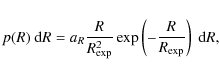
B00 obtained the already mentioned radial distribution of starforming
regions in the MW from the combined far infrared (FIR) and millimetric
emission produced by clusters of massive stars embedded in
ultra-compact HII regions. The FIR (surface)
luminosity, ![]() ,
has a Gaussian shaped rise until it reaches a maximum at
,
has a Gaussian shaped rise until it reaches a maximum at ![]() kpc
(FWHM of 2.38 kpc), then it decays
exponentially, with a scale-length of 1.78 kpc, towards the
outer part of the MW, approximately following the distribution
of neutral hydrogen. The radial birth probability is then obtained from
the FIR luminosity from the equation
kpc
(FWHM of 2.38 kpc), then it decays
exponentially, with a scale-length of 1.78 kpc, towards the
outer part of the MW, approximately following the distribution
of neutral hydrogen. The radial birth probability is then obtained from
the FIR luminosity from the equation
Another possible distribution of NS progenitors can be obtained from the surface density of Galactic SN remnants (Case & Battacharya 1998, hereafter CB98; see also Green 2005)
![\begin{displaymath}%
\rho(R) = \left(\frac{R}{R_{0}}\right)^{\alpha}\exp\left[-\frac{\beta(R-R_{0})}{R_{0}}\right],
\end{displaymath}](/articles/aa/full_html/2010/02/aa12222-09/img23.png)
|
(3) |
where
The fourth radial distribution adopted has been proposed
by F06
![\begin{displaymath}%
p(R) = \frac{1}{\sqrt{2\pi}\sigma}\exp\left[-\frac{(R-R_{\rm peak})^{2}}{2\sigma^{2}}\right],
\end{displaymath}](/articles/aa/full_html/2010/02/aa12222-09/img26.png)
|
(4) |
where
It is our opinion that the distribution proposed by P90, in spite of being obtained from observations of external galaxies, may better represent the long term star formation history of the MW. The other models are based on the present-day distribution of population I objects, which could have been rather different in past epochs (see for example Chiappini et al. 2001). The models of B00, CB90 and F06 are probably better suited for population studies of young/middle-aged NSs (PSRs, magnetars etc.).
![\begin{figure}
\par\includegraphics[width=8cm,clip]{12222fg1.ps}
\end{figure}](/articles/aa/full_html/2010/02/aa12222-09/img29.png)
|
Figure 1: Normalized radial probability distribution of NSs progenitors. P90 (solid line), B00 (dotted), CB98 (dashed) and F06 (dot-dashed). |
| Open with DEXTER | |
2.1.1 Spiral arms and initial distribution of heights
Massive stars are located in the spiral arms of the MW (they are indeed
the ideal tracers of the spiral structure), thus we model spiral arms
in the distribution of NS progenitors adopting the same prescription of
F06, i.e., NS progenitors are distributed along four
logarithmic spirals, each spiral described by the equation
The values of the parameters k, R* and
Table 1: Parameters of the spiral arms.
The thickness of the starforming region is few tens of parsecs (B00, Maiz-Apellaniz 2001). However, as P90 and Sun & Han (2004) have pointed out, the long term dynamical behavior of a NS population is insensitive to the scale height of its progenitors (see also Kiel & Hurley 2009). Following their results we assume that all NSs are born on the Galactic plane (z=0).
![\begin{figure}
\par\includegraphics[width=8cm,clip]{12222fg2.ps}
\end{figure}](/articles/aa/full_html/2010/02/aa12222-09/img32.png)
|
Figure 2: Initial positions of NSs - radial distribution from P90. The position of the Sun is (8.5, 0.0). |
| Open with DEXTER | |
2.2 Distribution of birth velocities
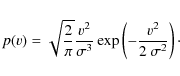
The true form of the distribution of birth velocities is still a hotly
debated issue and few constrains exist (see F06 for an
exhaustive discussion). HP97, L97 and H05 proposed a Maxwellian
distribution
|
(6) |
Alternatively, Fryer et al. (1998), Cordes & Chernoff (1998), A02 and B03 proposed a bimodal distribution
![\begin{displaymath}%
p(v) = \sqrt{\frac{2}{\pi}}~v^{2}~\left[ \frac{w}{\sigma_{1...
...^{3}}\exp\left(-\frac{v^{2}}{2~\sigma_{2}^{2}} \right)\right],
\end{displaymath}](/articles/aa/full_html/2010/02/aa12222-09/img34.png)
|
(7) |
where w is the relative weight of the two components of the distribution.
Using the same PSR sample of B03, F06 explored, together with
Maxwellian and bimodal models, other possible distribution functions
like the double-sided exponential
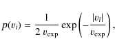
|
(8) |
where vi represents a single component of the velocity and
|
(9) |
where
|
(10) |
where again v represents the tridimensional velocity. F06 concluded that the Maxwellian model is less favored. On the other hand they disfavor also the bimodal distribution and prefer instead single parameter models, pointing out that the bimodality found by other authors arises if the alternative single parameter models are not investigated.
To explore the effects of the birth velocities on the final phase-space distribution of NSs, we adopt the Maxwellian model of H05 as well as four of the models proposed by F06, i.e. the bimodal, the double-sided exponential, the Lorentzian and that of P90. From here on we refer to these models as H05, F06B, F06E, F06L and F06P respectively.
The value of the mean tridimensional velocity for each
distribution is calculated numerically from simulated velocity vectors
(Table 2).
All the velocity distributions refer to the Local Standard of Rest
(LSR) of NS progenitors. Thus, the true 3D velocity
of a neutron star with respect to the Galactic Reference Frame (GRF) is
the vector sum of the birth velocity and the circular velocity at the
birthplace, ![]() .
.
![\begin{figure}
\par\includegraphics[width=8cm,clip]{12222fg3.ps}
\end{figure}](/articles/aa/full_html/2010/02/aa12222-09/img41.png)
|
Figure 3: Differential velocity distributions obtained from simulated velocity vectors. H05 (solid), F06DG (dotted), F06E (dashed), F06L (dot-dashed) and F06P (triple dot-dashed). |
| Open with DEXTER | |
Table 2: Velocity distribution models.
2.3 Gravitational potential
Once the initial conditions have been assigned, the motion of NSs is
described by the equation
where
| (12) |
where
The gravitational potential of the bulge is (Hernquist
1990)

|
(13) |
where
The disk potential has instead the following form (Miyamoto & Nagai 1975)
![\begin{displaymath}%
\Phi_{\rm D} = -\frac{GM_{\rm D}}{\sqrt{\left\{R^{2} + \left[R_{\rm D} + \sqrt{z_{\rm D}^2 + z^{2}}\right]^{2}\right\}}},
\end{displaymath}](/articles/aa/full_html/2010/02/aa12222-09/img61.png)
|
(14) |
where
Finally, the potential of the halo is (Navarro
et al. 1996)
|
(15) |
where
|
(16) |
is the characteristic density, c is the concentration parameter,
The parameters of potential are the same of S07, except for
the concentration parameter c and the
virial radius
![]() (19.2 and 274 kpc respectively), which were adjusted
to match the IAU standard values for the distance of the Sun from the
Galactic center, R0 =
8.5 kpc, and the circular velocity at the solar circle,
(19.2 and 274 kpc respectively), which were adjusted
to match the IAU standard values for the distance of the Sun from the
Galactic center, R0 =
8.5 kpc, and the circular velocity at the solar circle, ![]() =
=
![]() ,
together with the escape velocity from the MW at the same distance,
,
together with the escape velocity from the MW at the same distance, ![]()
![]()
![]() (S07). The
corresponding value of the virial mass,
(S07). The
corresponding value of the virial mass,
![]() ,
is
,
is
![]() .
.
Very recently Reid
et al. (2009) gave a new estimate of the circular
velocity, ![]() with
with ![]() ,
meaning that the MW may be more massive that previously thought.
To asses the effect of the enhanced mass of the Galaxy on
NS orbits, we choose a further set of parameters for the
potential: the masses of the bulge and disk are increased by a
factor
(254/220)2,
i.e. the ratio of the squared circular velocities in the two
cases. For the halo, the concentration parameter c
remains the same while the virial radius
,
meaning that the MW may be more massive that previously thought.
To asses the effect of the enhanced mass of the Galaxy on
NS orbits, we choose a further set of parameters for the
potential: the masses of the bulge and disk are increased by a
factor
(254/220)2,
i.e. the ratio of the squared circular velocities in the two
cases. For the halo, the concentration parameter c
remains the same while the virial radius
![]() is in this case 332 kpc, which yields an 80 percent
increase of the virial mass,
is in this case 332 kpc, which yields an 80 percent
increase of the virial mass, ![]()
![]() 1.8
1.8 ![]()
![]() .
.
We note that in the model where ![]() =
=
![]() we get
we get ![]() =
= ![]() .
This is higher than the central value (544 km s-1)
estimated by S07; however, it is not far from their
90% upper limit (608
.
This is higher than the central value (544 km s-1)
estimated by S07; however, it is not far from their
90% upper limit (608
![]() ), especially when we consider
that
), especially when we consider
that
![]() was obtained by assuming
was obtained by assuming ![]() =
= ![]() ,
and that modifying such assumption introduces further uncertainty in
its determination (Smith, private communication).
,
and that modifying such assumption introduces further uncertainty in
its determination (Smith, private communication).
![\begin{figure}
\par\includegraphics[width=8cm,clip]{12222fg4.ps}
\end{figure}](/articles/aa/full_html/2010/02/aa12222-09/img83.png)
|
Figure 4: Rotation curve for our Milky Way model (solid). Dotted, dashed and dot-dashed represent the bulge, disk and halo contributions respectively. |
| Open with DEXTER | |
![\begin{figure}
\par\includegraphics[width=8cm,clip]{12222fg5.ps}
\end{figure}](/articles/aa/full_html/2010/02/aa12222-09/img84.png)
|
Figure 5: Escape velocity on the Galactic plane. The circular velocity (dashed) is plotted for comparison. |
| Open with DEXTER | |
2.4 Orbit integration
We calculate the orbits of 150 000 NSs for each model (Table 3), assuming that NSs are born at constant rate during the whole MW lifetime (10 Gyr). Hence the age of each NS is selected randomly from an uniform distribution. The orbit of each NS is then calculated via numerical integration of Eq. (11), for a time corresponding to its assigned age. The axial symmetry of the potential implies conservation of angular momentum with respect to the axis of rotation of the MW. This allows to reduce the number of equations in (11) to four
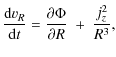

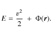
where jz is the angular momentum with respect to the z axis. Integration of Eqs. (17) is performed with a 4th order Runge-Kutta algorithm (e.g. Press et al. 1992) with customized adaptive stepsize. The relative accuracy of integrations is kept below 10-6 using the energy integral E as reference, i.e.
To limit the computation time
Table 3: Models for initial conditions.
3 Results
Our calculations show that the statistical properties of NSs are
affected mostly by the distribution of birth velocities while the
effects of different distributions of progenitors are less prominent.
For this reason we focus on results of models 1A
to 1E, i.e. with the distribution of progenitors
of P90. Results of models differing only for the distribution
of progenitors are quite similar, the only substantial difference is
the shape of the surface density (Fig. 6):
in fact, in models based on the
P90 progenitor distribution, the density peaks at the center (
![]() )
whereas for other models the density peaks off center (2
)
whereas for other models the density peaks off center (2 ![]()
![]()
![]() 6 kpc).
6 kpc).
![\begin{figure}
\par\includegraphics[width=8.5cm,clip]{12222fg6.ps}
\end{figure}](/articles/aa/full_html/2010/02/aa12222-09/img94.png)
|
Figure 6:
Surface density of NSs in the disk, obtained from best fit parameters (
|
| Open with DEXTER | |
3.1 Fraction of bound neutron stars
We first compute the fraction of NSs in bound orbits, ![]() .
Neglecting all those processes that could alter its energetic state
(e.g. two body interactions), the final fate of a NS
is known once its initial position and velocity are fixed.
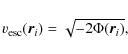
A NS star is bound when its initial velocity is lower
than the escape velocity at the birthplace,
.
Neglecting all those processes that could alter its energetic state
(e.g. two body interactions), the final fate of a NS
is known once its initial position and velocity are fixed.
A NS star is bound when its initial velocity is lower
than the escape velocity at the birthplace, ![]() , with
, with
|
(19) |
where
|
(20) |
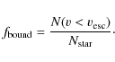
The retention fraction is
3.2 Distribution of heights
From here on our results are obtained rescaling ![]() from 150 000 to 109,
which is our reference value for the total number of NSs
produced in the MW.
from 150 000 to 109,
which is our reference value for the total number of NSs
produced in the MW.
Table 4: Statistical properties of NSs in the disk.
We study the distribution of NSs, f(z),
as a function of the height on the Galactic plane. We adopt a
logistic function
|
(21) |
as fitting function (see e.g. Fig. 7). From these fits we estimate the average half-density half-thickness z1/2 of the disk (Table 4). The values of the coefficients of the fit for each model, together with the corresponding maximum error, are listed in the Appendix (Table A.2). The half-density half-thickness shows substantial variations from model to model, going from 100 to
![\begin{figure}
\par\includegraphics[width=8.5cm,clip]{12222fg7.ps}
\end{figure}](/articles/aa/full_html/2010/02/aa12222-09/img109.png)
|
Figure 7: Distribution of heights f(z) - Model 1A. Dashed line represents the fitting function. |
| Open with DEXTER | |
3.3 Neutron stars in the disk
Here we define the Galactic disk as the cylindrical volume with radius
20 kpc and height 0.4 kpc (i.e. ![]() kpc
and
kpc
and ![]() kpc). The fraction
of NSs that reside in the disk,
kpc). The fraction
of NSs that reside in the disk,
![]() ,
goes from
,
goes from ![]() to
to ![]() .
Hence the majority of NSs born in the MW populate the halo
(Table 4).
.
Hence the majority of NSs born in the MW populate the halo
(Table 4).
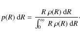
We fit the logarithmic surface density of the disk adopting a
fourth order polynomial as fitting function
|
(22) |
The accuracy of these fits is always better than 5 percent. The values of the coefficients aj are listed in the Appendix (Table A.1).
We made a visual check of the final distribution of NSs in the disk, looking for traces of the spiral arms. We found no evidence of spiral structure in the evolved distribution (compare Figs. 8 and 2).
![\begin{figure}
\par\includegraphics[width=8cm,clip]{12222fg8.ps}
\end{figure}](/articles/aa/full_html/2010/02/aa12222-09/img115.png)
|
Figure 8: Final distribution of NSs in the disk - Model 1E*. |
| Open with DEXTER | |
The hypothesis of constant formation rate yields an average age of ![]() Gyr,
with young/middle-aged (<10 Myr) NSs representing only
Gyr,
with young/middle-aged (<10 Myr) NSs representing only ![]() percent
of the whole population.
As expected this value is higher inside the disk,
by a factor
percent
of the whole population.
As expected this value is higher inside the disk,
by a factor ![]() 10, since NSs are born there, and did not have
enough time to run away. However the excess of young NSs
(Fig. 9)
does not alter the mean age in the disk, which is also
10, since NSs are born there, and did not have
enough time to run away. However the excess of young NSs
(Fig. 9)
does not alter the mean age in the disk, which is also ![]() Gyr.
Gyr.
![\begin{figure}
\par\includegraphics[width=8cm,clip]{12222fg9.ps}
\end{figure}](/articles/aa/full_html/2010/02/aa12222-09/img118.png)
|
Figure 9: Distribution of ages - Model 1A. Solid an dashed lines represent global and disk populations respectively. |
| Open with DEXTER | |
3.3.1 Mean velocities
The mean velocity of NSs in the disk is roughly the same for all
models, ![]()
![]()
![]() in the GRF while in the LSR the mean velocity is lower,
in the GRF while in the LSR the mean velocity is lower, ![]()
![]()
![]() .
An exception are models based on the distribution F06P, which
show mean velocities in the LSR of
.
An exception are models based on the distribution F06P, which
show mean velocities in the LSR of ![]() .
This fact can be easily explained: in the F06P model
low birth velocities have higher probability
(see Fig. 3)
and thus the main contributor to the velocity of the star is the
circular velocity,
.
This fact can be easily explained: in the F06P model
low birth velocities have higher probability
(see Fig. 3)
and thus the main contributor to the velocity of the star is the
circular velocity, ![]()
![]()
![]() .
.
The low velocity in the LSR implies also that NSs can not move too far away from the disk and this is the reason why, for models F06P, the scale height is considerably lower than in other models.
Following Z95, we fit the cumulative velocity distribution of
NSs, both with respect to the GRF and the LSR, with the following
function
|
(23) |
where a v0 is a characteristic velocity. Fit values for v0, m and n are listed in the Appendix (Tables A.3 and A.4).
3.3.2 The solar neighbourhood
To compare our results with previous works we focus now on the
statistical properties of NSs in the so-called solar region,
7.5 ![]() R
R ![]() 9.5 kpc, as in BR, BM and Z95.
9.5 kpc, as in BR, BM and Z95.
From the fits we discussed in the previous subsection, we
obtain the local surface density
![]() which varies from
which varies from ![]()
![]()
![]() .
The volume density in the solar vicinity, n0,
also varies by a factor 5 between models, from
.
The volume density in the solar vicinity, n0,
also varies by a factor 5 between models, from ![]()
![]() 10-4
10-4
![]() .
.
We can now infer the distance of the nearest NS simply by
computing the minimum volume around the Sun which contains at least
a NS, assuming constant density
|
(24) |
typical values of
Table 5: Statistical properties of NSs at the solar circle.
3.4 Halo neutron stars
![\begin{figure}
\par\includegraphics[width=8.5cm,clip]{12222fg10.ps}
\end{figure}](/articles/aa/full_html/2010/02/aa12222-09/img134.png)
|
Figure 10: Model 1A - ( upper panel) radial distribution of NSs in the halo. ( lower panel) Mean velocity. |
| Open with DEXTER | |
The distribution of NSs in the halo is shown in Fig. 10. Bound NSs can
be found as far as ![]() 1.5 Mpc,
however the majority lies within the virial radius of the MW (
1.5 Mpc,
however the majority lies within the virial radius of the MW (
![]() ).
The radial distribution clearly shows that unbound NSs start to be
dominant at
).
The radial distribution clearly shows that unbound NSs start to be
dominant at ![]() 500 kpc.
Accordingly the mean velocity, after an initial drop, starts to rise
almost linearly from
500 kpc.
Accordingly the mean velocity, after an initial drop, starts to rise
almost linearly from ![]() 500 kpc.
The gravitational effects of other galaxies (e.g. Andromeda
and the Magellanic Clouds) have not been considered.
500 kpc.
The gravitational effects of other galaxies (e.g. Andromeda
and the Magellanic Clouds) have not been considered.
3.5 Density maps
We compute the projected number density of NSs in heliocentric coordinates (l, b, d) and give the relative sky maps for stars within 30, 10 and 3 kpc respectively. Our sky maps (Fig. 12) clearly show that the most promising direction to look for NSs is towards the Galactic center, where the density is higher. Moving away from the center, the density drops rapidly even along the Galactic plane (Fig. 11).
In Table 6
we list the inferred values of the projected density towards specific
lines of sight (LOS). The sampling distance varies according to the
LOS: for example, towards the GC the sampling distance, ![]() ,
is equal to R0 while
for the three other LOS lying on the Galactic plane
,
is equal to R0 while
for the three other LOS lying on the Galactic plane
![]() is equal to the distance at which the LOS itself crosses the outer
border of the stellar disk (20 kpc).
is equal to the distance at which the LOS itself crosses the outer
border of the stellar disk (20 kpc).
For large values of ![]() the projected density has non-negligible values even at high Galactic
latitudes. One intriguing consequence is that NSs in the halo may
contribute to the observable rate of microlensing events, both of
Galactic and extragalactic sources (Sartore et al.,
in preparation). We thus calculate also the expected number
density of NSs in the direction of the Magellanic Clouds,
assuming 48 and 61 kpc for distance of the Large and
Small Magellanic Clouds respectively (Table 6).
the projected density has non-negligible values even at high Galactic
latitudes. One intriguing consequence is that NSs in the halo may
contribute to the observable rate of microlensing events, both of
Galactic and extragalactic sources (Sartore et al.,
in preparation). We thus calculate also the expected number
density of NSs in the direction of the Magellanic Clouds,
assuming 48 and 61 kpc for distance of the Large and
Small Magellanic Clouds respectively (Table 6).
Table 6: Projected density of NSs towars different lines of sight.
![\begin{figure}
\par\includegraphics[width=8cm,clip]{12222fg11a.ps}\vspace*{5mm}
\includegraphics[width=8cm,clip]{12222fg11b.ps}
\end{figure}](/articles/aa/full_html/2010/02/aa12222-09/img148.png)
|
Figure 11:
Density profile on the Galactic plane (b=0,
upper panel) and along a meridian (l=0,
lower panel) for |
| Open with DEXTER | |
![\begin{figure}
\par\includegraphics[width=8.5cm,clip]{12222fg12a.ps}\vspace*{2mm...
....ps}\vspace*{2mm}
\includegraphics[width=8.5cm,clip]{12222fg12c.ps}
\end{figure}](/articles/aa/full_html/2010/02/aa12222-09/img149.png)
|
Figure 12:
Sky maps of the projected density (
|
| Open with DEXTER | |
3.6 Results with different potential
Calculations made with the updated potential are labelled with an
asterisk in the tables and give the following results. The retention
fraction
![]() exhibits a significant increase, especially for models 1A*
and 1C*, while for the remaining ones the enhancement is less
conspicuous.
In all cases the fraction of NSs retained by the disk is only slightly
increased (Table 4).
exhibits a significant increase, especially for models 1A*
and 1C*, while for the remaining ones the enhancement is less
conspicuous.
In all cases the fraction of NSs retained by the disk is only slightly
increased (Table 4).
In all models with the updated potential, the scale height of the population is lower due to the increased masses of the disk and bulge, the decrease in z1/2 being of the order of 10-20 percent (see the half-density half-thickness in Table 4).
The higher number of NSs retained by the disk implies also higher values of the surface and volume densities, together with the projected density for LOSs in the Galactic plane. For the same reason, even relatively fast NSs can be found in the disk, thus increasing the mean velocities on NSs (see Tables 4 and 5).
4 Discussion
Our calculations show that the distribution of birth velocities is the
main factor driving the dynamics of NSs in the MW. We obtain
substantially different values of
![]() among different birth velocity models, with the shape of the
distribution (position of the peak, bimodality, etc.) also
playing a role in determining the final fate of bound NSs.
among different birth velocity models, with the shape of the
distribution (position of the peak, bimodality, etc.) also
playing a role in determining the final fate of bound NSs.
The highest escape fraction, ![]() ,
are obtained with H05, F06E and F06L distributions. This value
is lower than those found by Lyne &
Lorimer (1994,
hereafter LL) and A02 and similar to that inferred
by H05. This is probably due to the fact that the
velocity distributions proposed by LL and A02 were obtained adopting
the distribution of free electrons of Taylor
& Cordes (1993). Both H05 and F06 adopted
instead the revised model of Cordes
& Lazio (2002) for free electrons, which reduced
estimates for distance, and thus velocity, of young pulsars. We
performed a run with the distribution of A02, obtaining
,
are obtained with H05, F06E and F06L distributions. This value
is lower than those found by Lyne &
Lorimer (1994,
hereafter LL) and A02 and similar to that inferred
by H05. This is probably due to the fact that the
velocity distributions proposed by LL and A02 were obtained adopting
the distribution of free electrons of Taylor
& Cordes (1993). Both H05 and F06 adopted
instead the revised model of Cordes
& Lazio (2002) for free electrons, which reduced
estimates for distance, and thus velocity, of young pulsars. We
performed a run with the distribution of A02, obtaining ![]()
![]() 0.54, confirming their results on the escape fraction.
0.54, confirming their results on the escape fraction.
The adoption of the updated potential (higher mass of the
Galaxy) implies higher escape velocities and hence only the
fastest NSs, ![]() percent,
can definitely escape from the MW.
percent,
can definitely escape from the MW.
Albeit more than 70 percent of the NSs born in the MW are in
bound orbits, the present-day number of NSs in the disk is only a small
fraction of the total, ![]() .
The remaining ones are found in the halo where they spend most of their
life. This is a striking result but was not totally unexpected
because, given their high spatial velocities, our
synthetic NSs leave the disk in a short timescale,
.
The remaining ones are found in the halo where they spend most of their
life. This is a striking result but was not totally unexpected
because, given their high spatial velocities, our
synthetic NSs leave the disk in a short timescale, ![]() Myr.
Another remarkable finding is that the ratio of young to old NSs in the
disk is very low: for each neutron star detected as a
young active source there should be still more than 100 old
NSs hiding in the disk.
Myr.
Another remarkable finding is that the ratio of young to old NSs in the
disk is very low: for each neutron star detected as a
young active source there should be still more than 100 old
NSs hiding in the disk.
Our simulated NSs are born with significantly higher
velocities with respect to what is found in other works.
In spite of this, our results for the half density half
thickness show no significant differences with previous studies (except
for the F06P distribution). Also, the local spatial density of NSs
falls between those found by BR, BM, Z95 and that of P90,
i.e. approximately between 1 and 5 ![]()
![]() .
This means that the nearest neutron star lies within
.
This means that the nearest neutron star lies within ![]() pc
from the Sun.
pc
from the Sun.
The mean velocity is higher by at least a factor ![]() with respect to, for example, that found by BR, BM
and Z95. Low velocity NSs (v
with respect to, for example, that found by BR, BM
and Z95. Low velocity NSs (v ![]()
![]() )
in the disk are a tiny fraction, f50
)
in the disk are a tiny fraction, f50 ![]() 0.001.
This fraction grows by a factor
0.001.
This fraction grows by a factor ![]() in the LSR where
in the LSR where ![]() is
is
![]() .
Again results obtained with the F06P distribution show a rather
different behavior, with f50
.
Again results obtained with the F06P distribution show a rather
different behavior, with f50 ![]() 0.01 in the GRF while in the LSR roughly half of NSs in the disk are in
the low velocity tail (Tables 4 and 5). However, the
effective weight of the low velocity tail of the distribution of birth
velocities is still matter for debate.
0.01 in the GRF while in the LSR roughly half of NSs in the disk are in
the low velocity tail (Tables 4 and 5). However, the
effective weight of the low velocity tail of the distribution of birth
velocities is still matter for debate.
Most of NSs, both bound and unbound, run away from the
Galactic plane in a short timescale and form a halo which extends well
beyond the virial radius of the MW. The phase-space
distribution of halo NSs clearly shows a separation between bound and
unbound NSs. Unbound NSs become dominant at r ![]() 500 kpc.
500 kpc.
The results presented in this paper will enable us to revisit a number of problems concerning isolated old NSs, like the accretion luminosity and its observability, the strategies for observing very close NSs, say within 100 pc and the optical depth of NSs in the perspective of using gravitational lensing to probe the population.
Note added in proof After this manuscript was accepted, we became aware of a similar work by Ofek (2009, PASP, 121, 814). His results are somewhat different from ours, probably due to the different set of initial conditions adopted in his model.
AcknowledgementsWe thank the anonymous referee for several helpful comments which improved the previous versions of this paper. We thank also M. C. Smith for helpful suggestions on the parameters of the Milky Way potential. N.S. wishes to thank R. Salvaterra for useful comments on the manuscript and L. Paredi for technical support. The work of RT is partially supported by INAF/ASI through grant AAE-I/088/06/0.
Appendix A: Coefficients of the fits
We give here the best fit parameters for the surface density of the disk (Table A.1), the height distribution (Table A.2) and the cumulative velocity distributions in the disk, both in the GRF (Table A.3) and in the LSR (Table A.4).
Table A.1: Surface density of the disk.
Table A.2: Distribution of heights.
Table A.3: Cumulative velocity distribution in the disk.
Table A.4: Cumulative velocity distribution in the disk (LSR).
References
- Arzoumanian, Z., Chernoff, D. F., & Cordes, J. M. 2002, ApJ, 568, 289 (A02) [NASA ADS] [CrossRef] [Google Scholar]
- Binney, J., & Tremaine, S. 1987, Galactic Dynamics (Princeton: Princeton Univ. Press) [Google Scholar]
- Blaaw, A. 1961, Bull. Astron. Inst. Netherlands, 15, 265 [NASA ADS] [Google Scholar]
- Blaes, O., & Madau, P. 1993, ApJ, 403, 690 (BM) [NASA ADS] [CrossRef] [Google Scholar]
- Blaes, O., & Rajagopal, M. 1991, ApJ, 381, 210 (BR) [NASA ADS] [CrossRef] [Google Scholar]
- Brisken, W. F., Fruchter, A. S., Goss, W. M., Herrnestein, R. M., & Thorsett, S. E. 2003, AJ, 126, 3090 (B03) [NASA ADS] [CrossRef] [Google Scholar]
- Bronfman, L., Casassus, S., May, J., & Nyman, L.-Å. 2000, A&A, 358, 521 (B00) [NASA ADS] [Google Scholar]
- Case, G. L., & Battacharya, D. 1998, ApJ, 504, 761 (CB98) [Google Scholar]
- Chatterjee, S., Vlemmings, W. H. T., Brisken, W. F., et al. 2005, ApJ, 630, L61 [NASA ADS] [CrossRef] [Google Scholar]
- Chiappini, C., Matteucci, F., & Romano, D. 2001, ApJ, 554, 1044 [NASA ADS] [CrossRef] [Google Scholar]
- Cordes, J. M., & Chernoff, D. F. 1998, ApJ, 505, 315 (CC) [NASA ADS] [CrossRef] [Google Scholar]
- Cordes, J. M., & Lazio, T. J. W. 2002, NE2001. I. A New Model for the Galactic distribution of Free Electrons and Its Fluctuations [Google Scholar]
- Dewey, R. J., & Cordes, J. M. 1987, ApJ, 321, 780 [NASA ADS] [CrossRef] [Google Scholar]
- Diehl, R., Halloin, H., Kretschmer, K., et al. 2006, Nature, 439, 45 [NASA ADS] [CrossRef] [PubMed] [Google Scholar]
- Faucher-Giguere, C., & Kaspi, V. M. 2006, ApJ, 643, 332 (F06) [NASA ADS] [CrossRef] [Google Scholar]
- Fryer, C., Burrows, A., & Benz, W. 1998, ApJ, 496, 333 [NASA ADS] [CrossRef] [Google Scholar]
- Green, D. A. 2005, MmSAI, 76, 534 [Google Scholar]
- Gvaramadze, V. V., Gualandris, A., & Portegies Zwart, S. 2008, MNRAS, 385, 929 [NASA ADS] [CrossRef] [Google Scholar]
- Hansen, B. M. S., & Phinney, E. S. 1997, MNRAS, 291, 569 (HP97) [NASA ADS] [Google Scholar]
- Hartman, J. W. 1997, A&A, 322, 127 [NASA ADS] [Google Scholar]
- Hartmann, D., Epstein, R. I., & Woosley, S. E. 1990, ApJ, 348, 625 (H90) [NASA ADS] [CrossRef] [Google Scholar]
- Hernquist, L. 1990, ApJ, 356, 359 [NASA ADS] [CrossRef] [Google Scholar]
- Hobbs, G., Lorimer, D. R., Lyne, A. G., & Kramer, M. 2005, MNRAS, 360, 974 (H05) [NASA ADS] [CrossRef] [Google Scholar]
- Hui, C. Y., & Becker, W. 2006 A&A, 457, L33 [Google Scholar]
- Iben, I. Jr., & Tutukov, A. V. 1996, ApJ, 456, 738 [NASA ADS] [CrossRef] [Google Scholar]
- Keane, E. F., & Kramer, M. 2008, MNRAS, 391, 209 [Google Scholar]
- Kiel, P. D., & Hurley, J. R. 2006, MNRAS, 369, 1152 [NASA ADS] [CrossRef] [Google Scholar]
- Kiel, P. D., & Hurley, J. R. 2009, MNRAS, 395, 2326 [NASA ADS] [CrossRef] [Google Scholar]
- Kiel, P. D., Hurley, J. R., Bailes, M., & Murray, J. R. 2008, MNRAS, 388, 393 [NASA ADS] [CrossRef] [Google Scholar]
- Kuijken, K., & Gilmore, G. 1989, MNRAS, 239, 651 [NASA ADS] [Google Scholar]
- Lorimer, D. R. 2008, Living Rev. Relativity, 11, 8 [Google Scholar]
- Lorimer, D. R., Bailes, M., & Harrison, P. A. 1997, MNRAS, 289, 592 (L97) [NASA ADS] [Google Scholar]
- Lyne, A. G., & Lorimer, D. R. 1994, Nature, 369, 127 (LL) [NASA ADS] [CrossRef] [Google Scholar]
- Lyne, A. G., Anderson, B., & Salter, M. J. 1982, MNRAS, 213, 613 [Google Scholar]
- Maíz-Apellániz, J. 2001, AJ, 121, 2737 [Google Scholar]
- Miyamoto, M., & Nagai, R. 1975, PASJ, 27, 533 [NASA ADS] [Google Scholar]
- Motch, C., Pires, A. M., Haberl, F., Schwope, A., & Zavlin, V. E. 2009, A&A, 497, 423 [NASA ADS] [CrossRef] [EDP Sciences] [Google Scholar]
- Narayan, R., & Ostriker, J. P. 1990, ApJ, 352, 222 [NASA ADS] [CrossRef] [Google Scholar]
- Navarro, J. F., Frenk, C. S., & White, S. D. M. 1996, ApJ, 462, 563 [NASA ADS] [CrossRef] [Google Scholar]
- Neuhauser, R., & Trumper, J. E. 1999, A&A, 343, 151 [NASA ADS] [Google Scholar]
- Paczynski, B. 1990, ApJ, 348, 485 (P90) [NASA ADS] [CrossRef] [Google Scholar]
- Popov, S. B., & Prokhorov, M. E. 1998, A&A, 331, 55 (PP98) [Google Scholar]
- Popov, S. B., Colpi, M., Treves, A., et al. 2000, ApJ, 530, 896 (P00) [NASA ADS] [CrossRef] [Google Scholar]
- Popov, S. B., Colpi, M., Prokhorov, M. E., Treves, A., & Turolla, R. 2003, A&A, 406, 111 [NASA ADS] [CrossRef] [EDP Sciences] [Google Scholar]
- Popov, S. B., Turolla, R., Prokhorov, M. E., Colpi, M., & Treves, A. 2005, Ap&SS, 299, 117 [NASA ADS] [CrossRef] [Google Scholar]
- Press, W. H., Teukolsky, S. A., Vetterling, W. T., & Flannery, B. P. 1992, Numerical recipes, 2nd edn. (Cambridge: Cambridge University Press) [Google Scholar]
- Reid, M. J., Menten, K. M., Zheng, X. W., et al. 2009, ApJ, 700, 137 [NASA ADS] [CrossRef] [Google Scholar]
- Shklovskii, I. S. 1970, SvA, 13, 562 [Google Scholar]
- Smith, M. C., Ruchti, G. R., Helmi, A., et al. 2007, MNRAS, 379, 755 (S07) [NASA ADS] [CrossRef] [Google Scholar]
- Sun, X. H., & Han, J. L. 2004, MNRAS, 350, 232 [NASA ADS] [CrossRef] [Google Scholar]
- Taylor, J. H., & Cordes, J. M. 1993, ApJ, 411, 674 [NASA ADS] [CrossRef] [Google Scholar]
- Treves, A., Turolla, R., Zane, S., & Colpi, M. 2000, PASP, 112, 297 [NASA ADS] [CrossRef] [Google Scholar]
- van der Kruit, P. C. 1987, in The Galaxy, Series C: Mathematical and Physical Sciences, ed. G. Gilmore, & R. Carswell (Dordrecht: Reidel), 207 [Google Scholar]
- Xue, X. X., Rix, H. W., Zhao, G., et al. 2008, ApJ, 684, 1143 [NASA ADS] [CrossRef] [Google Scholar]
- Yusiforv, I., & Kucuk, I. 2004, A&A, 422, 545 [NASA ADS] [CrossRef] [EDP Sciences] [Google Scholar]
- Zane, S., Turolla, R., Zampieri, L., Colpi, M., & Treves, A. 1995, ApJ, 451, 739 (Z95) [NASA ADS] [CrossRef] [Google Scholar]
Footnotes
- ... accretors
![[*]](/icons/foot_motif.png)
- No sources have been positively identified so far.
- ... brightness
- In th J band.
- ... time
- The CPU time for a typical run is about 1 day.
All Tables
Table 1: Parameters of the spiral arms.
Table 2: Velocity distribution models.
Table 3: Models for initial conditions.
Table 4: Statistical properties of NSs in the disk.
Table 5: Statistical properties of NSs at the solar circle.
Table 6: Projected density of NSs towars different lines of sight.
Table A.1: Surface density of the disk.
Table A.2: Distribution of heights.
Table A.3: Cumulative velocity distribution in the disk.
Table A.4: Cumulative velocity distribution in the disk (LSR).
All Figures
|
|
Figure 1: Normalized radial probability distribution of NSs progenitors. P90 (solid line), B00 (dotted), CB98 (dashed) and F06 (dot-dashed). |
| Open with DEXTER | |
| In the text | |
|
|
Figure 2: Initial positions of NSs - radial distribution from P90. The position of the Sun is (8.5, 0.0). |
| Open with DEXTER | |
| In the text | |
|
|
Figure 3: Differential velocity distributions obtained from simulated velocity vectors. H05 (solid), F06DG (dotted), F06E (dashed), F06L (dot-dashed) and F06P (triple dot-dashed). |
| Open with DEXTER | |
| In the text | |
|
|
Figure 4: Rotation curve for our Milky Way model (solid). Dotted, dashed and dot-dashed represent the bulge, disk and halo contributions respectively. |
| Open with DEXTER | |
| In the text | |
|
|
Figure 5: Escape velocity on the Galactic plane. The circular velocity (dashed) is plotted for comparison. |
| Open with DEXTER | |
| In the text | |
|
|
Figure 6:
Surface density of NSs in the disk, obtained from best fit parameters (
|
| Open with DEXTER | |
| In the text | |
|
|
Figure 7: Distribution of heights f(z) - Model 1A. Dashed line represents the fitting function. |
| Open with DEXTER | |
| In the text | |
|
|
Figure 8: Final distribution of NSs in the disk - Model 1E*. |
| Open with DEXTER | |
| In the text | |
|
|
Figure 9: Distribution of ages - Model 1A. Solid an dashed lines represent global and disk populations respectively. |
| Open with DEXTER | |
| In the text | |
|
|
Figure 10: Model 1A - ( upper panel) radial distribution of NSs in the halo. ( lower panel) Mean velocity. |
| Open with DEXTER | |
| In the text | |
|
|
Figure 11:
Density profile on the Galactic plane (b=0,
upper panel) and along a meridian (l=0,
lower panel) for |
| Open with DEXTER | |
| In the text | |
|
|
Figure 12:
Sky maps of the projected density (
|
| Open with DEXTER | |
| In the text | |
Copyright ESO 2010
Current usage metrics show cumulative count of Article Views (full-text article views including HTML views, PDF and ePub downloads, according to the available data) and Abstracts Views on Vision4Press platform.
Data correspond to usage on the plateform after 2015. The current usage metrics is available 48-96 hours after online publication and is updated daily on week days.
Initial download of the metrics may take a while.