| Issue |
A&A
Volume 509, January 2010
|
|
|---|---|---|
| Article Number | A21 | |
| Number of page(s) | 7 | |
| Section | Stellar structure and evolution | |
| DOI | https://doi.org/10.1051/0004-6361/200913332 | |
| Published online | 12 January 2010 | |
First spectroscopic analysis of  Scorpii C and Scorpii E
Discovery of a new HgMn star in the multiple system Scorpii
G. Catanzaro
INAF - Osservatorio Astrofisico di Catania, via S. Sofia 78, 95123 Catania, Italy
Received 21 September 2009 / Accepted 8 October 2009
Abstract
Context. The multiple system ![]() Scorpii consists of five components and two suspected members forming a
total of seven stars. In the past, this system acquired much interest
because of a series of occultation by the planet Jupiter and one of its
satellites (Io). The study of this phenomena allowed us to
ascertain the principal components of the system and the possible
nature of each component.
Scorpii consists of five components and two suspected members forming a
total of seven stars. In the past, this system acquired much interest
because of a series of occultation by the planet Jupiter and one of its
satellites (Io). The study of this phenomena allowed us to
ascertain the principal components of the system and the possible
nature of each component.
Aims. By using optical spectroscopy, we derive radial velocities,
![]() ,
,
![]() ,
abundances
,
abundances ![]() ,
,
![]() ,
and
,
and ![]() for
for ![]() Sco C and E. We also refine previously published values of
Sco C and E. We also refine previously published values of ![]() ,
,
![]() ,
and
,
and ![]() of
of ![]() Sco Aa + Ab to obtain a clear understanding of the evolutionary state of the
Sco Aa + Ab to obtain a clear understanding of the evolutionary state of the ![]() Sco system.
Sco system.
Methods. We convert Doppler shifts in wavelength into radial
velocities. Atmospheric parameters and abundances are computed by
assuming the local thermodynamic equilibrium using model atmospheres
and the spectral synthesis codes ATLAS and SYNTHE.
Results. We solve the orbit of ![]() Sco E and provide information about the motion of
Sco E and provide information about the motion of ![]() Sco C. By fitting four Balmer lines, we determine that:
Sco C. By fitting four Balmer lines, we determine that:
![]() K,
K,
![]() ,
and
,
and
![]() K,
K,
![]() .
Rotational velocities are derived by modeling the profiles of metallic lines:
.
Rotational velocities are derived by modeling the profiles of metallic lines:
![]() km s-1 and
km s-1 and
![]() km s-1. As for the abundances, we find that
km s-1. As for the abundances, we find that ![]() Sco C is more or less of solar abundance, while
Sco C is more or less of solar abundance, while ![]() Sco Ea
has a significant overabundance of manganese, followed by those of
strontium, phosphorous, and titanium. The most underabundant element is
magnesium, followed by silicon, aluminum, sulfur, iron, and nickel.
Other light elements, such as carbon, nitrogen, oxygen, and neon, are
found to be normal. From the derived values of luminosities and
temperatures, we infer that these stars have an age of
Sco Ea
has a significant overabundance of manganese, followed by those of
strontium, phosphorous, and titanium. The most underabundant element is
magnesium, followed by silicon, aluminum, sulfur, iron, and nickel.
Other light elements, such as carbon, nitrogen, oxygen, and neon, are
found to be normal. From the derived values of luminosities and
temperatures, we infer that these stars have an age of ![]()
![]() Myr.
Myr.
Conclusions. We explain the observed variability in velocity of ![]() Sco E in terms of a close companion. Thus, we observe a triple system composed by
Sco E in terms of a close companion. Thus, we observe a triple system composed by ![]() Sco C and
Sco C and ![]() Sco Ea + Eb. While
Sco Ea + Eb. While ![]() Sco C is a normal star,
Sco C is a normal star, ![]() Sco Ea is probably a mercury-manganese (HgMn) star. The line-profile variability observed for
Sco Ea is probably a mercury-manganese (HgMn) star. The line-profile variability observed for ![]() Sco C
could be explained by assuming its membership to the class of slow
pulsating B stars. According to the position of
Sco C
could be explained by assuming its membership to the class of slow
pulsating B stars. According to the position of ![]() Sco Ab in the HR diagram, we exclude the possibility that this star could be a
Sco Ab in the HR diagram, we exclude the possibility that this star could be a ![]() Cephei class pulsator.
Cephei class pulsator.
Key words: stars: individual: ![]() Scorpii - binaries: spectroscopic - stars: abundances - stars: chemically peculiar
Scorpii - binaries: spectroscopic - stars: abundances - stars: chemically peculiar
1 Introduction
![]() Scorpii is one of the most remarkable multiple systems in all the
northern sky. Its components have been studied extensively since 1964,
when a sequence of occultations by planet Jupiter occurred. The most detailed
description of the system was given by Van Flandern & Espenschied (1975) and a couple
of years later by Evans et al. (1977). After these studies, no additional observations
have been made.
Scorpii is one of the most remarkable multiple systems in all the
northern sky. Its components have been studied extensively since 1964,
when a sequence of occultations by planet Jupiter occurred. The most detailed
description of the system was given by Van Flandern & Espenschied (1975) and a couple
of years later by Evans et al. (1977). After these studies, no additional observations
have been made.
Before continuing, we summarize the properties of the system and the
nomenclature of its component. Component A is HD 144217
(HR 5984), a B0.5 V star with
V = 2.62 (Nicolet 1978). It was found by Abhyankar (1959) to be a
spectroscopic binary (Aa + Ab) with
![]() (Elliot et al. 1976) and an orbital period of
(Elliot et al. 1976) and an orbital period of
![]() days (Holmgren at al. 1997).
Components Aa + Ab have a more distant companion, the
B component. It has been a visual companion since the middle of
the last century when its slow orbital motion
brought it too close to A for visual separation. According to Evans et al. (1977),
the separation between A and B is approximately of 0.394 arcsec. Van Flandern & Espenschied (1975)
also detected a possible spectroscopic companion to B, on the
basis that the B component should have a mass greater than that deduced from its
assumed absolute magnitude, to ensure the dynamical stability of the
system. However, this component (G) has yet to be confirmed.
days (Holmgren at al. 1997).
Components Aa + Ab have a more distant companion, the
B component. It has been a visual companion since the middle of
the last century when its slow orbital motion
brought it too close to A for visual separation. According to Evans et al. (1977),
the separation between A and B is approximately of 0.394 arcsec. Van Flandern & Espenschied (1975)
also detected a possible spectroscopic companion to B, on the
basis that the B component should have a mass greater than that deduced from its
assumed absolute magnitude, to ensure the dynamical stability of the
system. However, this component (G) has yet to be confirmed.
Holmgren at al. (1997) studied ![]() Sco A in detail with the twofold purpose of
searching for line profile variability (LPV) and to provide more accurate physical
parameters of the components. They found for Aa and Ab, respectively,
the following atmospheric parameters:
Sco A in detail with the twofold purpose of
searching for line profile variability (LPV) and to provide more accurate physical
parameters of the components. They found for Aa and Ab, respectively,
the following atmospheric parameters:
![]() K
and
K
and
![]() = 3.95
= 3.95 ![]() 0.33 (B0.5IV-V),
0.33 (B0.5IV-V),
![]() = 26 400
= 26 400 ![]() 2000 K and
2000 K and
![]() = 4.20
= 4.20 ![]() 0.35
(B1.5 V). They also proposed that
0.35
(B1.5 V). They also proposed that ![]() Sco Ab could be a
Sco Ab could be a ![]() Cep-type
star, since they claimed a possible LPV detection with a period of
0.17333 days. Finally, from their analysis the authors suggested the
presence of eclipses.
Cep-type
star, since they claimed a possible LPV detection with a period of
0.17333 days. Finally, from their analysis the authors suggested the
presence of eclipses.
Far from the A component, the component C (HD 144218 = HR 5985) lies at a
distance estimated by Van Flandern & Espenschied (1975) to be 13.6 arcsec; it is a B2 V
star with V = 4.92 (Johnson & Morgan 1953). The analysis used to study data for the
occultation by the Jupiter satellite Io, found this star to be double, its E
component with a difference of 2.1 mag (Evans et al. 1977) having a very close separation of ![]() 0.1 arcsec (Bartholdi & Owen 1972; Hubbard & Van Flandern 1972). Basing their argument on its unusual colors, Van Flandern & Espenschied (1975)
suggested that this component should itself be double, and proposed
that its hypothetical companion as F, or alternatively that it
could be a peculiar star with no additional companion.
0.1 arcsec (Bartholdi & Owen 1972; Hubbard & Van Flandern 1972). Basing their argument on its unusual colors, Van Flandern & Espenschied (1975)
suggested that this component should itself be double, and proposed
that its hypothetical companion as F, or alternatively that it
could be a peculiar star with no additional companion.
The orbital elements of the visual couples AB (BU 947AB) and CE (McA 42CE) were computed for the first time by Seymour et al. (2002), who found periods of 610 yrs and 28.1 yrs, respectively. These authors stated that the orbits of two-component pairs of this complex system were calculated independently of each another and a multibody solution was not attempted.
For the CE pair, no detailed spectroscopic analysis has yet been performed to our knowledge.
The aim of this paper is to characterize these two stars, their motions and their
atmospheres, deriving their effective temperatures, gravities, and abundances. In
particular, this study will allow us to draw some important conclusions about the
possible presence of the F companion. Further, because of the Holmgren at al. (1997)
parallaxes, we could refine the astrophysical quantities such as:
![]() ,
,
![]() ,
and
,
and ![]() ,
of all the principal four components of
,
of all the principal four components of ![]() Sco system, and we discuss the Holmgren at al. (1997) hypothesis regarding the membership of
Sco system, and we discuss the Holmgren at al. (1997) hypothesis regarding the membership of ![]() Sco Ab to the class of
Sco Ab to the class of ![]() Cephei pulsators.
Cephei pulsators.
2 Observations and data reduction
The spectra used in our analysis were acquired with different equipments:
- a spectrum of Sco C + E was downloaded from the ESO
archive. In particular, this spectrum was acquired with
FEROS@MPI-2.2 m on May 3, 2004 at La Silla Observatory, Chile.
The signal-to-noise ratio was always higher than 150.
The spectral resolution was
R = 48 000.
- Spectrum of the pair Sco C + E
were downloaded from the CFHT archive. This spectrum was acquired on
May 20, 2005 with ESPADONS mounted on the 3.6 m and covers a
wavelength region from 3750 to 9200 Å, a signal-to-noise ratio
always greater than 300. Because of the strong contamination by
telluric lines and the presence of fringes, we limited our analysis to
the interval between 3700 Å and 7000 Å. Resolving power is
 70 000, as
derived from emission lines of the Th-Ar calibration lamp.
70 000, as
derived from emission lines of the Th-Ar calibration lamp.
- The 91 cm telescope of the INAF - Osservatorio
Astrofisico di Catania (OAC), was used by ourselves to acquire 13
spectra of Sco C + E. The telescope is fiber-linked to a REOSC echelle spectrograph, which allows us to obtain
R = 20 000 spectra in the range
4300-6800 Å. The resolving was measured using emission
lines of the Th-Ar calibration lamp. Spectra were recorded on a thinned, back-illuminated (SITE) CCD with
 pixels of 24
  m size, a typical readout noise of 6.5 e-, and a gain of 2.5 e-/ADU.
3 Radial velocities and orbital parameters
In our highest resolution spectra (i.e., CFHT and ESO), the lines of
the E component are easily detected at a wide range of wavelengths.
Unfortunately, because of their lower resolution, in the OAC data we
identified the lines of that component only in the limited fraction of
the spectral range between 4545 Å and 4580 Å. In particular,
we identified 5 lines, namely: Cr II ![]() 4558.650 Å,
Ti II
4558.650 Å,
Ti II ![]() 4563.757, Ti II
4563.757, Ti II ![]() 4571.971,
Fe II
4571.971,
Fe II ![]() 4583.837, and Cr II
4583.837, and Cr II ![]() 4588.199. For each of these lines, we measured the central wavelength
with a Gaussian fit of the profile and computed the radial velocity
using the classical Doppler shift formula. Velocities are reported in
Table 1.
4588.199. For each of these lines, we measured the central wavelength
with a Gaussian fit of the profile and computed the radial velocity
using the classical Doppler shift formula. Velocities are reported in
Table 1.
Table 1: Radial velocities derived from our spectra.
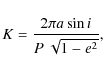
The radial velocities of a spectroscopic binary system are linked to the orbital parameters by the relation:
where
|
(2) |
where P is the orbital period of the system. Orbital elements were determined by a least-square fit to Eq. (1). Errors were estimated from the variation in the parameters which increases the
Table 2: Orbital parameters calculated for the E components.
![\begin{figure}
\par\includegraphics[width=9cm,clip]{13332fg1.ps}\vspace{-3mm}
\vspace*{1.5mm}
\vspace{-3mm}\end{figure}](/articles/aa/full_html/2010/01/aa13332-09/img38.png)
|
Figure 1:
Radial velocity curves of |
| Open with DEXTER | |
Regarding ![]() Sco C, we were unable to fit the data to Eq. (1) and noted that the OAC data infers, within the experimental errors, the same
velocity, whose average value is
Sco C, we were unable to fit the data to Eq. (1) and noted that the OAC data infers, within the experimental errors, the same
velocity, whose average value is
![]() .
.
The visual couple CE, also known as McA 42CE, has an orbital period of ![]() 28.1 yrs (Seymour et al. 2002). We found that the E component has an orbital motion with a
P = 10.6851 days. Thus, these results could be interpreted
in the framework of a new scenario, in which the C component is
physically linked to a close binary system consisting of
28.1 yrs (Seymour et al. 2002). We found that the E component has an orbital motion with a
P = 10.6851 days. Thus, these results could be interpreted
in the framework of a new scenario, in which the C component is
physically linked to a close binary system consisting of ![]() Sco Ea + Eb.
Sco Ea + Eb.
4 Atmospheric parameters of the components
The approach that we used in this study to determine
![]() and
and ![]() of
of ![]() Sco C and
Sco C and ![]() Sco Ea, was applied in Catanzaro & Leone (2006)
to the triple system 74 Aqr. It consists of comparing the observed and
theoretical profiles of all Balmer lines available in our spectra by minimizing the goodness-of-fit parameter
Sco Ea, was applied in Catanzaro & Leone (2006)
to the triple system 74 Aqr. It consists of comparing the observed and
theoretical profiles of all Balmer lines available in our spectra by minimizing the goodness-of-fit parameter
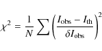
where N is the total number of points,
The synthetic spectrum normalized to the unity level was derived using the
formula
where
Theoretical single profiles were computed with SYNTHE (Kurucz & Avrett 1981) on the basis
of ATLAS9 (Kurucz 1993) atmosphere models. All models were evaluated for a
solar opacity distribution function and microturbulence velocity ![]() km s-1.
To reduce the number of free parameters, we first determined the rotational
velocities of
km s-1.
To reduce the number of free parameters, we first determined the rotational
velocities of ![]() Sco C
and Ea by matching metal lines to synthetic profiles in our
highest resolution (CFHT) spectra. The best-fit occurred for the
values reported in Table 3.
Sco C
and Ea by matching metal lines to synthetic profiles in our
highest resolution (CFHT) spectra. The best-fit occurred for the
values reported in Table 3.
Table 3: Atmospheric parameters adopted in our study for the components of our system.
For our purpose, we used only the CFHT spectrum, which is
the one of the highest resolution and signal-to-noise ratio (SNR) among
our data. We extracted four Balmer lines, namely H![]() ,
H
,
H![]() ,
H
,
H![]() ,
and H
,
and H![]() ,
where the SNR measured in the continuum next to the wings varies from 250 to 300.
,
where the SNR measured in the continuum next to the wings varies from 250 to 300.
The results obtained by applying this procedure are presented in Table 3 and displayed in Fig. 2. The values obtained for the C component agree with the B2V classification reported in literature.
![\begin{figure}
\par\includegraphics[width=9cm,clip]{13332fg2.ps}\vspace*{1.5mm}
\end{figure}](/articles/aa/full_html/2010/01/aa13332-09/img52.png)
|
Figure 2:
Comparison between observed (CFHT) and computed Balmer line profiles. The synthetic total profile is the combination of |
| Open with DEXTER | |
5 Abundance analysis
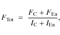
To derive chemical abundances, we undertook a synthetic modeling of the observed spectrum. This is because of the intrinsic difficulty in determining the true equivalent widths of metal lines that are strongly reduced by the dilution effect caused by the superposition of the fluxes of the components.
In practice, we divided the entire spectral range
covered by our data into a number of subintervals each of 20 Å wide. For each interval, we derived the abundances by a ![]() minimization of the
difference between the observed and synthetic total spectrum.
Line lists and atomic parameters used in our modeling are taken from
Kurucz & Bell (1995) and the subsequent update by Castelli & Hubrig (2004).
minimization of the
difference between the observed and synthetic total spectrum.
Line lists and atomic parameters used in our modeling are taken from
Kurucz & Bell (1995) and the subsequent update by Castelli & Hubrig (2004).
Table 4:
Abundances derived for ![]() Sco C + Ea expressed in term of
Sco C + Ea expressed in term of
![]() compared with the solar values of Asplund et al. (2005).
compared with the solar values of Asplund et al. (2005).
In Table 4, we report the abundances derived in our analysis
expressed in the usual logarithmic form relative to the total number of
atoms
![]() .
To easily compare the chemical pattern of
.
To easily compare the chemical pattern of ![]() Sco C + E,
we report in the last column the solar abundances taken from Asplund et al. (2005)
Sco C + E,
we report in the last column the solar abundances taken from Asplund et al. (2005)![]() . Error reported in Table 4
for a given element is the standard deviation of the average computed
among the various abundances determined in each subinterval. When a
given element appears in one or two sub-intervals
only, the error in its abundance evaluated by varying temperature and
gravity in the ranges
. Error reported in Table 4
for a given element is the standard deviation of the average computed
among the various abundances determined in each subinterval. When a
given element appears in one or two sub-intervals
only, the error in its abundance evaluated by varying temperature and
gravity in the ranges
![]() and
and
![]() is typically 0.20 dex. The abundances of both
objects are displayed in Fig. 3.
is typically 0.20 dex. The abundances of both
objects are displayed in Fig. 3.
![\begin{figure}
\par\includegraphics[width=8.8cm,clip]{13332fg3.ps}\vspace*{1.5mm}
\end{figure}](/articles/aa/full_html/2010/01/aa13332-09/img61.png)
|
Figure 3: Abundance patterns for the two components. Open circles (blue) represent the pattern of the C component, filled circles (red) are relative to the Ea component. |
| Open with DEXTER | |
To check the accuracy of our
![]() and
and ![]() values
determined for the C component, we could consider the consistency
of the abundances derived from spectral lines of silicon in the first two
stages of ionization:
values
determined for the C component, we could consider the consistency
of the abundances derived from spectral lines of silicon in the first two
stages of ionization:
![]() for Si II and
for Si II and
![]() for Si III.
for Si III.
In the following sections, we discuss the abundances derived for each component. For each star, we comment on the results for light elements (from carbon to sulfur), iron-group elements (from scandium to nickel) and heavy elements, if any. Regarding helium, spectral lines of the two components are so strongly blended to each other that the measurement of its abundance is impossible.
5.1 Sco C
Regarding the light elements reported in Table 4,
we did not find any particular peculiarity,
only a very slight overabundance of neon and magnesium (![]() 0.5 dex each).
0.5 dex each).
For what that concerns iron-group elements, we found spectral lines of iron
that led to an abundance of -4.92 ![]() 0.16, slightly beneath the solar value.
0.16, slightly beneath the solar value.
Thus, on the basis of our analysis we conclude that this object can be considered as a normal star, as can easily be noted in Fig. 3.
From a visual examination of the spectra in the Si III triplet region,
we noted a clear line-profile variation similar to those expected for radial
and non-radial pulsations. As an example, we show in Fig. 4
the Si III
![]() 4567-4574 Å lines for five spectra taken from our sample. To make
this comparison possible, we deconvolved the highest resolution data
(ESO and CFHT) to the resolution of the OAC resolving power spectra. We
attempt to provide an interpretation of this phenomenon in Sect. 7.
4567-4574 Å lines for five spectra taken from our sample. To make
this comparison possible, we deconvolved the highest resolution data
(ESO and CFHT) to the resolution of the OAC resolving power spectra. We
attempt to provide an interpretation of this phenomenon in Sect. 7.
![\begin{figure}
\par\includegraphics[width=8.8cm,clip]{13332fg4.ps}
\end{figure}](/articles/aa/full_html/2010/01/aa13332-09/img65.png)
|
Figure 4:
Example data of the Si III 4567 and 4574 Å of |
| Open with DEXTER | |
5.2 Sco Ea
Carbon, nitrogen and oxygen were found to have normal abundances, in addition to neon. Strong underabundances, between 1.0 and 1.5 dex, were found for magnesium, aluminum, silicon, and sulfur, while phosphorus shows an abundance of 0.5 dex greater than the solar case.
For iron-group elements, we found solar abundances for only
scandium and chromium. Overabundances were inferred for both titanium
(slight, ![]() 0.5 dex) and manganese (strong,
0.5 dex) and manganese (strong, ![]() 2.0 dex). Only iron and nickel have abundances of below solar,
2.0 dex). Only iron and nickel have abundances of below solar, ![]() 1.0 and
1.0 and ![]() 0.8 dex,
respectively.
0.8 dex,
respectively.
In our spectrum, we inferred the presence of only one element
heavier than nickel, i.e., strontium, for which an overabundance of
![]() 0.8 dex was computed.
0.8 dex was computed.
The chemical pattern of the E component is very complicated, as the reader can see in Fig. 3. It seems to combine a number of abundance anomalies that usually appear in various classes of chemically peculiar stars.
The first hypothesis is that we are dealing with a HgMn star,
since it shows clear overabundances of manganese and strontium. Unfortunately,
the Hg II 3984 Å
line, which is the principal indicator of this class of peculiarity, is
confused with a much stronger blend (O II 3982.714 plus S III 3983.722 Å) belonging to the component C. This allow us to
estimate only an upper limit to the mercury overabundance of ![]() 3.5 dex, otherwise the line would have been detected.
3.5 dex, otherwise the line would have been detected.
On the other hand, underabundance of elements such as magnesium, silicon,
phosphorous, and iron, are typical of other classes of peculiarity, such as
![]() Boo stars for instance, rather than HgMn stars.
Boo stars for instance, rather than HgMn stars.
![\begin{figure}
\par\includegraphics[width=18cm,clip]{13332fg5.ps}
\end{figure}](/articles/aa/full_html/2010/01/aa13332-09/img66.png)
|
Figure 5:
As for example, we show four different intervals of CFHT spectra superimposed on the computed model. Dotted (cyan) line
represent the synthetic spectrum computed for the C component, dashed
(green) line is the synthetic spectrum calculated for the E component,
while the total model is represented by the solid heavy (red) line. In these
plots, we also identify the spectral lines with the atomic number and
ionization states of the chemical element that generates the line, i.e.,
25.01 means Mn II. The labels above the spectrum refer to |
| Open with DEXTER | |
6 Fundamental astrophysical quantities
The parallax found by Holmgren at al. (1997) for the Aa + Ab pair provides
us with the opportunity to refine the positions of these fours stars on
the HR diagram. Moreover, since ![]() Sco C and
Sco C and ![]() Sco Ea belong to the same stellar system, we also adopted the same distance for these two stars.
Sco Ea belong to the same stellar system, we also adopted the same distance for these two stars.
For the effective temperatures, we adopted those estimated in the study of
![]() Sco C and
Sco C and ![]() Sco Ea and those published by Holmgren at al. (1997)
for the pair Aa + Ab, that is
Sco Ea and those published by Holmgren at al. (1997)
for the pair Aa + Ab, that is
![]() = 28 000
= 28 000 ![]() 2000 K and
2000 K and
![]() = 26 400
= 26 400 ![]() 2000 K.
2000 K.
We determine their luminosities on the basis of: visual magnitudes taken from
Holmgren at al. (1997) for Aa + Ab and from Mason et al. (2001) for the C + Ea couple; the Sun's bolometric magnitude
![]() (Drilling & Landolt 1999); the BC from the calibrations published by Flower (1996); and the extinction
coefficients Av of de Geus et al. (1989). Input data and the obtained luminosities are reported in Table 5.
(Drilling & Landolt 1999); the BC from the calibrations published by Flower (1996); and the extinction
coefficients Av of de Geus et al. (1989). Input data and the obtained luminosities are reported in Table 5.
Table 5:
Astrophysical quantities for the ![]() Sco System.
Sco System.
The absolute radii reported in Table 5 were estimated as follows: for the components Aa, Ab, and C we directly combined the angular diameters measured by Elliot et al. (1976) and Elliot et al. (1975) with the adopted distance, while for the Ea components, since no direct measurement of its angular size is available in the literature, we estimated the radius using both the luminosity and effective temperature.
The mass-luminosity relation of main-sequence stars,
![]() (Drilling & Landolt 1999), has been used to derive the mass of each component.
(Drilling & Landolt 1999), has been used to derive the mass of each component.
With our values of
![]() and L, we constructed the HR diagram
showed in Fig. 6. A comparison with the evolutionary tracks
of Bressan et al. (1993), computed for Z = 0.02 (solar metalicity),
and with isochrones computed by Bertelli et al. (1994)
indicates for the
and L, we constructed the HR diagram
showed in Fig. 6. A comparison with the evolutionary tracks
of Bressan et al. (1993), computed for Z = 0.02 (solar metalicity),
and with isochrones computed by Bertelli et al. (1994)
indicates for the ![]() Sco system an age of
Sco system an age of ![]() 6.3
6.3 ![]() 3.0 Myr,
which agrees with the value found by Giannuzzi (1983).
3.0 Myr,
which agrees with the value found by Giannuzzi (1983).
7 Discussion and conclusion
The present study represents the first ever quantitative spectroscopic analysis of the stars ![]() Sco C and
Sco C and ![]() Ea. By using ATLAS9 models with
Ea. By using ATLAS9 models with
![]() K,
K,
![]() for
for ![]() Sco C, and
Sco C, and
![]() K,
K,
![]() for
for ![]() Sco Ea (both with
Sco Ea (both with ![]() km s-1),
we have computed a composite synthetic spectrum and compared it with
the observed spectrum. The atmospheric parameters have been computed by
a fitting approach that involved at the same time the composite
profiles of four Balmer lines, namely: H
km s-1),
we have computed a composite synthetic spectrum and compared it with
the observed spectrum. The atmospheric parameters have been computed by
a fitting approach that involved at the same time the composite
profiles of four Balmer lines, namely: H![]() ,
H
,
H![]() ,
H
,
H![]() ,
and H
,
and H![]() (see Fig. 2).
(see Fig. 2).
According to our analysis, the C component has almost solar metalicity. From the results of the previous section, it can be seen that this component falls into the correct ranges of spectral types and masses to be a suitable candidate slow pulsating B-star (SPBs) (Waelkens 1991). This could explain the lines profile variability evident in Fig. 4. Of course, since we do have insufficient data to search for a periodicity, this conclusion needs to be verified by increasing the amount of high resolution spectra at our disposal.
![\begin{figure}
\par\includegraphics[width=9cm,clip]{13332fg6.ps}\vspace{2mm}
\end{figure}](/articles/aa/full_html/2010/01/aa13332-09/img75.png)
|
Figure 6:
Positions on the HR diagram of the |
| Open with DEXTER | |
The most puzzling star is certainly component Ea: it exhibits typical
characteristics of the HgMn peculiarity class, i.e., strong
overabundances of manganese and strontium, but at the same time strong
underabundances of other elements such as magnesium, silicon, sulfur,
and iron that are usually normal or overabundant in HgMn stars.
Nevertheless, this particular chemical composition is not an isolated
case in the literature. The pattern that we show in Fig. 3 is very similar to that derived for HR 6000, another HgMn star,
studied in detail by Catanzaro et al. (2004) and Castelli & Hubrig (2007).
The latter authors tried to explain its peculiarity by considering
chemical stratification within the atmosphere. A similar study is
difficult to perform in ![]() Sco Ea because of the spectral contamination of the C component.
Sco Ea because of the spectral contamination of the C component.
As a final conclusion about their atmospherical parameters, we state that
![]() Sco C is a standard star, while
Sco C is a standard star, while ![]() Sco Ea is a chemically peculiar object far more likely to belong to the HgMn subgroup.
Sco Ea is a chemically peculiar object far more likely to belong to the HgMn subgroup.
In Sect. 3, we derived the orbital parameters of ![]() Sco Ea (Table 2) by fitting the observed radial velocities to Eq. (1). As we showed there, we were unable to perform the same fitting of
Sco Ea (Table 2) by fitting the observed radial velocities to Eq. (1). As we showed there, we were unable to perform the same fitting of ![]() Sco C velocities, since the entire set
of OAC data do not show any appreciable variability, at least at our resolving power.
Sco C velocities, since the entire set
of OAC data do not show any appreciable variability, at least at our resolving power.
Van Flandern & Espenschied (1975) proposed
two explanations of the unusual colors of the E component: a close
companion or a very peculiar chemical composition. Our results seem to
be in favor of both hypotheses, that is a chemically peculiar star (![]() Sco Ea) with a close companion (
Sco Ea) with a close companion (![]() Sco Eb).
Sco Eb).
Holmgren at al. (1997) attempted a preliminary search for line profile variability in the spectral lines of ![]() Sco Ab, detecting a possible period of 0.17333 days. They proposed that the star belongs to the class of
Sco Ab, detecting a possible period of 0.17333 days. They proposed that the star belongs to the class of ![]() Cephei pulsators.
Cephei pulsators.
![]() Cephei
stars are early-B type, near main-sequence objects, which exhibit
variations in brightness, radial velocity, and line profiles on
timescales of several hours, due to radial and non-radial p- and g-mode
pulsations. They are located on the HR diagram in a narrow region where
the classic k-mechanism is effective in the partial ionization zone of
the iron-group elements. They are in the late stages of core
hydrogen-burning phase, just preceding the secondary gravitational
contraction (Balona & Engelbrecht 1981).
For a clear look at their location inside the instability region, we
address the reader to the HR diagram of the confirmed and candidate
Cephei
stars are early-B type, near main-sequence objects, which exhibit
variations in brightness, radial velocity, and line profiles on
timescales of several hours, due to radial and non-radial p- and g-mode
pulsations. They are located on the HR diagram in a narrow region where
the classic k-mechanism is effective in the partial ionization zone of
the iron-group elements. They are in the late stages of core
hydrogen-burning phase, just preceding the secondary gravitational
contraction (Balona & Engelbrecht 1981).
For a clear look at their location inside the instability region, we
address the reader to the HR diagram of the confirmed and candidate ![]() Cephei stars published by Stankov & Handler (2005).
Cephei stars published by Stankov & Handler (2005).
According to our results, ![]() Sco Ab is far from the instability region
(see Fig. 6),
so we do not confirm the conclusion drawn by previous authors, and, if
it exists, the line profile variability has to be ascribed to another
origin, such as for example the SPB phenomenon.
Sco Ab is far from the instability region
(see Fig. 6),
so we do not confirm the conclusion drawn by previous authors, and, if
it exists, the line profile variability has to be ascribed to another
origin, such as for example the SPB phenomenon.
This research has made use of the SIMBAD database, operated at CDS, Strasbourg, France. This research has made use of the Washington Double Star Catalog maintained at the US Naval Observatory.Based on observations made with ESO Telescopes at the La Silla Observatories under programme ID 073.C-0337. This research used the facilities of the Canadian Astronomy Data Centre operated by the National Research Council of Canada with the support of the Canadian Space Agency.
A warm thanks to Anna for her contribution in improving the English form of the manuscript.
References
- Abhyankar, V. D. 1959, ApJS, 4, 157 [NASA ADS] [CrossRef] [Google Scholar]
- Asplund, M., Grevesse, N., & Sauval, A. J. 2005, in Cosmic Abundances as Records of Stellar Evolution and Nucleosynthesis, ASP Conf. Ser., 336, 25 [Google Scholar]
- Balona, L. A., & Engelbrecht, C. 1981, in Workshop on Pulsating B stars, ed. G. E. V. O. N., & C. Sterken, Nice Observatory, 195 [Google Scholar]
- Bartholdi, P., & Owen, F. 1972, AJ, 77, 60 [NASA ADS] [CrossRef] [Google Scholar]
- Bertelli, G., Bressan, A., Chiosi, C., Fagotto, F., & Nasi, E. 1994, A&AS, 106, 275 [Google Scholar]
- Bressan, A., Fagotto, F., Bertelli, G., et al. 1993, A&AS, 100, 647 [Google Scholar]
- de Geus, E. J., de Zeeuw, P. T., & Lub, J. 1989, A&A, 216, 44 [Google Scholar]
- Catanzaro, G., & Leone, F. 2006, MNRAS, 373, 330 [NASA ADS] [CrossRef] [Google Scholar]
- Catanzaro, G., Leone, F., & Dall, T. H. 2004, A&A, 425, 641 [Google Scholar]
- Castelli, F., & Hubrig, S. 2004, A&A, 425, 263 [Google Scholar]
- Castelli, F., & Hubrig, S. 2007, A&A, 475, 1041 [Google Scholar]
- Drilling, J. S., & Landolt, A. U. 1999, in Allen's Astrophysical Quantities, fourth edition, ed. A. N. Cox, Los Alamos, NM, 381 [Google Scholar]
- Elliot, J. L., Wasserman, L. H., Veverka, J., Sagan, C., & Liller, W. 1975, AJ, 80, 323 [NASA ADS] [CrossRef] [Google Scholar]
- Elliot, J. L., Rages, K., & Veverka, J. 1976, ApJ, 207, 994 [NASA ADS] [CrossRef] [Google Scholar]
- Evans, D. S., Africano, J. L., Fekel, F. C., et al. 1977, AJ, 82, 495 [NASA ADS] [CrossRef] [Google Scholar]
- Flower, P. J. 1996, ApJ, 469, 355 [NASA ADS] [CrossRef] [Google Scholar]
- Giannuzzi, M. A. 1983, A&A, 125, 302 [Google Scholar]
- Johnson, H. L., & Morgan, W. W. 1953, ApJ, 117, 313 [NASA ADS] [CrossRef] [Google Scholar]
- Harmanec, P., Hadrava, P., Yang, S., et al. 1997, A&A, 319, 867 [Google Scholar]
- Holmgren, D., Hadrava, P., Harmanec, P., Koubský, P., & Kubát, J. 1997, A&A, 322, 565 [Google Scholar]
- Hubbard, W. B., & Van Flandern, T. C. 1972, AJ, 77, 65 [NASA ADS] [CrossRef] [Google Scholar]
- Kurucz, R. L. 1993, A new opacity-sampling model atmosphere program for arbitrary abundances, in Peculiar versus normal phenomena in A-type and related stars, IAU Coll. 138, ed. M. M. Dworetsky, F. Castelli, & R. Faraggiana, ASP Conf. Ser., 44, 87 [Google Scholar]
- Kurucz, R. L., & Avrett, E. H. 1981, SAO Special Rep., 391 [Google Scholar]
- Kurucz, R. L., & Bell, B. 1995, Kurucz CD-ROM No. 23, Cambridge, Mass.: Smithsonian Astrophysical Observatory [Google Scholar]
- Nicolet, B. 1978, A&AS, 34, 1 [Google Scholar]
- Mason, B. D., Wycoff, G. L., Hartkopf, W. I., Douglass, G. G., & Worley C. E. 2001, AJ, 122, 3466 [Google Scholar]
- Seymour, D. M., Mason, B. D., Hartkopf, W. I., et al. 2002, AJ, 123, 1023 [NASA ADS] [CrossRef] [Google Scholar]
- Stankov, A., & Handler, G. 2005, ApJS, 158, 193 [NASA ADS] [CrossRef] [Google Scholar]
- Stellingwerf, R. F. 1978, ApJ, 224, 953 [NASA ADS] [CrossRef] [Google Scholar]
- Van Flandern, T. C., & Espenschied, P. 1975, ApJ, 200, 61 [NASA ADS] [CrossRef] [Google Scholar]
- Waelkens, C. 1991, A&A, 246, 453 [Google Scholar]
Footnotes
- ...Asplund et al. (2005)
![[*]](/icons/foot_motif.png)
- To ensure that these values are directly comparable with
our abundances, we changed the scale
 relative to
  ,
to the scale relative to
,
to the scale relative to  .
.
All Tables
Table 1: Radial velocities derived from our spectra.
Table 2: Orbital parameters calculated for the E components.
Table 3: Atmospheric parameters adopted in our study for the components of our system.
Table 4:
Abundances derived for ![]() Sco C + Ea expressed in term of
Sco C + Ea expressed in term of
![]() compared with the solar values of Asplund et al. (2005).
compared with the solar values of Asplund et al. (2005).
Table 5:
Astrophysical quantities for the ![]() Sco System.
Sco System.
All Figures
|
|
Figure 1:
Radial velocity curves of |
| Open with DEXTER | |
| In the text | |
|
|
Figure 2:
Comparison between observed (CFHT) and computed Balmer line profiles. The synthetic total profile is the combination of |
| Open with DEXTER | |
| In the text | |
|
|
Figure 3: Abundance patterns for the two components. Open circles (blue) represent the pattern of the C component, filled circles (red) are relative to the Ea component. |
| Open with DEXTER | |
| In the text | |
|
|
Figure 4:
Example data of the Si III 4567 and 4574 Å of |
| Open with DEXTER | |
| In the text | |
|
|
Figure 5:
As for example, we show four different intervals of CFHT spectra superimposed on the computed model. Dotted (cyan) line
represent the synthetic spectrum computed for the C component, dashed
(green) line is the synthetic spectrum calculated for the E component,
while the total model is represented by the solid heavy (red) line. In these
plots, we also identify the spectral lines with the atomic number and
ionization states of the chemical element that generates the line, i.e.,
25.01 means Mn II. The labels above the spectrum refer to |
| Open with DEXTER | |
| In the text | |
|
|
Figure 6:
Positions on the HR diagram of the |
| Open with DEXTER | |
| In the text | |
Copyright ESO 2010
Current usage metrics show cumulative count of Article Views (full-text article views including HTML views, PDF and ePub downloads, according to the available data) and Abstracts Views on Vision4Press platform.
Data correspond to usage on the plateform after 2015. The current usage metrics is available 48-96 hours after online publication and is updated daily on week days.
Initial download of the metrics may take a while.