| Issue |
A&A
Volume 509, January 2010
|
|
|---|---|---|
| Article Number | A67 | |
| Number of page(s) | 9 | |
| Section | Atomic, molecular, and nuclear data | |
| DOI | https://doi.org/10.1051/0004-6361/200913040 | |
| Published online | 20 January 2010 | |
The fate of S-bearing species after ion irradiation of interstellar icy grain mantles
M. Garozzo1 - D. Fulvio1,2 - Z. Kanuchova1,3 - M. E. Palumbo1 - G. Strazzulla1
1 - INAF - Osservatorio Astrofisico di Catania, via S. Sofia 78, 95123 Catania, Italy
2 - Dipartimento di Fisica e Astronomia, Università di Catania, Italy
3 - Astronomical Institute of Slovak Academy of Science, 059 60, T. Lomnica, Slovakia
Received 31 July 2009 / Accepted 8 October 2009
Abstract
Context. Chemical models predict the presence of S-bearing molecules such as hydrogen sulfide (H2S)
in interstellar icy grain mantles in dense molecular clouds. Up to now
only two S-bearing molecules, namely sulfur dioxide (SO2)
and carbonyl sulfide (OCS), have been detected in the solid phase
towards young stellar objects (YSOs), while upper limits for solid H2S
have been reported towards the same lines of sight. The estimated
abundance of S-bearing molecules in icy grain mantles is not able to
account for the cosmic S abundance.
Aims. In this paper we studied the effects of ion irradiation on different icy targets formed by carbon monoxide (CO) and SO2 or H2S as mixtures and, for the first time, as layers.
Methods. We carried out several irradiation experiments on ices containing SO2 or H2S mixed or layered with CO. The samples were irradiated with 200 keV protons in a high-vacuum chamber (
P < 10-7 mbar) at a temperature of
16-20 K. IR spectra of the samples were recorded after
various steps of irradiation and after warm-up.
Results. We have found that the column density of H2S and SO2, as well as CO, decreases after irradiation, and the formation of new molecular species is observed. In the case of CO:SO2 samples, OCS, sulfur trioxide (SO3), ozone (O3), and carbon dioxide (CO2) are the most abundant species formed. In the case of CO:H2S samples the most abundant species formed are OCS, SO2, carbon disulfide (CS2), hydrogen persulfide (H2S2), and CO2. The profile of the OCS band formed after irradiation of the CO:H2S mixture compares well with the profile of the OCS band detected towards the high mass YSO W33A.
Conclusions. Our results show that on a time scale comparable to the molecular cloud lifetime, the column density of H2S
is strongly reduced and we suggest that this could explain the failure
of its detection in the solid phase in the lines of sight of YSOs. We
suggest that the solid OCS and SO2 detected in dense molecular clouds are formed after ion irradiation of icy grain mantles.
Key words: astrochemistry - molecular processes - methods: laboratory - techniques: spectroscopic, ISM: molecules - ISM: abundances
1 Introduction
Observations of various astrophysical environments show that ices are
very common in the Universe. They can be found in the Solar System (on
the surface of planets, satellites, comets and other minor objects), as
well as in the interstellar medium, inside dense molecular clouds
where,
due to the low temperature (![]() 10 K) and high density (
10 K) and high density (![]() 104 H cm-3),
gas species freeze out on dust grains forming icy mantles. When the
ices are exposed to particle fluxes (cosmic ions, solar wind, etc.),
they are modified chemically and structurally. Incoming ions release
their energy into the target and destroy molecular bonds producing
fragments that, by recombination, form new molecules, also different
from the original ones and, in general, also with a new lattice
structure. This explains the change of spectral behavior of irradiated
surfaces (Brunetto et al. 2006) as well as the chemical composition of cometary (e.g. Strazzulla et al. 1991) or interstellar (e.g. Palumbo et al. 2000)
ices. Thus, the laboratory simulations of ion irradiation on different
materials (ices) is key in understanding their evolution within the
Solar System and in the interstellar medium. In this paper, we have
focused on the study of the alterations induced by cosmic ion
bombardment of S-bearing molecules in the icy mantles of dust grains in
dense molecular clouds.
Until now, only two S-bearing molecules - sulfur dioxide (SO2) and carbonyl sulfide (OCS) - have been detected in icy grain mantles (e.g. Boogert et al. 1996,1997; Zasowski et al. 2009; Palumbo et al. 1995,1997), while the presence of hydrogen sulfide (H2S) has been suggested (e.g. Geballe et al. 1985) although it has never been firmly identified, probably because its main band near 3.92
104 H cm-3),
gas species freeze out on dust grains forming icy mantles. When the
ices are exposed to particle fluxes (cosmic ions, solar wind, etc.),
they are modified chemically and structurally. Incoming ions release
their energy into the target and destroy molecular bonds producing
fragments that, by recombination, form new molecules, also different
from the original ones and, in general, also with a new lattice
structure. This explains the change of spectral behavior of irradiated
surfaces (Brunetto et al. 2006) as well as the chemical composition of cometary (e.g. Strazzulla et al. 1991) or interstellar (e.g. Palumbo et al. 2000)
ices. Thus, the laboratory simulations of ion irradiation on different
materials (ices) is key in understanding their evolution within the
Solar System and in the interstellar medium. In this paper, we have
focused on the study of the alterations induced by cosmic ion
bombardment of S-bearing molecules in the icy mantles of dust grains in
dense molecular clouds.
Until now, only two S-bearing molecules - sulfur dioxide (SO2) and carbonyl sulfide (OCS) - have been detected in icy grain mantles (e.g. Boogert et al. 1996,1997; Zasowski et al. 2009; Palumbo et al. 1995,1997), while the presence of hydrogen sulfide (H2S) has been suggested (e.g. Geballe et al. 1985) although it has never been firmly identified, probably because its main band near 3.92 ![]() m overlaps with a feature of methanol (CH3OH). The gaseous OCS molecules observed in hot cores are thought to have originated on dust grains (Hatchell et al. 1998). The parent molecules of OCS are not yet known. Ferrante et al. (2008) recently suggested that OCS is a product of ion irradiation of a mixture of CO and H2S ice. For our study, we carried out several irradiation experiments on ices containing SO2 and H2S
pure or mixed with carbon monoxide (CO). Although models of
interstellar ices propose that their compounds are mixed together,
recent observations suggest that interstellar ices are best represented
by a layered ice model rather than mixed ice (Fraser et al. 2004; Palumbo 2006).
For this reason, we have performed experiments with different kinds of
icy targets. Some targets were prepared by a co-deposition of a mixture
of two gas compounds at low temperature (CO and SO2 or H2S) and others by a deposition of an SO2 or H2S
layer subsequently covered with a CO layer. The substrate for the
experiments was a silicon wafer or a KBr pellet.
To our knowledge, the layered ones are the first experiments ever
performed to study the chemistry induced at the interface between two
icy species, while irradiation experiments with different gases and gas
mixtures deposited on a refractory substrate at low temperature are
more common (Mennella et al. 2004; Gomis & Strazzulla 2005,2008; Moore et al. 2007a; Loeffler et al. 2006).
Details of all the experiments performed and discussed in this work are listed in Table 1. The thickness of all the targets was smaller than the penetration depth of the used ions (200 keV H+);
so, after the energy release into the material, the passing ions were
implanted in the (silicon or KBr) substrate on which ices had been
deposited.
m overlaps with a feature of methanol (CH3OH). The gaseous OCS molecules observed in hot cores are thought to have originated on dust grains (Hatchell et al. 1998). The parent molecules of OCS are not yet known. Ferrante et al. (2008) recently suggested that OCS is a product of ion irradiation of a mixture of CO and H2S ice. For our study, we carried out several irradiation experiments on ices containing SO2 and H2S
pure or mixed with carbon monoxide (CO). Although models of
interstellar ices propose that their compounds are mixed together,
recent observations suggest that interstellar ices are best represented
by a layered ice model rather than mixed ice (Fraser et al. 2004; Palumbo 2006).
For this reason, we have performed experiments with different kinds of
icy targets. Some targets were prepared by a co-deposition of a mixture
of two gas compounds at low temperature (CO and SO2 or H2S) and others by a deposition of an SO2 or H2S
layer subsequently covered with a CO layer. The substrate for the
experiments was a silicon wafer or a KBr pellet.
To our knowledge, the layered ones are the first experiments ever
performed to study the chemistry induced at the interface between two
icy species, while irradiation experiments with different gases and gas
mixtures deposited on a refractory substrate at low temperature are
more common (Mennella et al. 2004; Gomis & Strazzulla 2005,2008; Moore et al. 2007a; Loeffler et al. 2006).
Details of all the experiments performed and discussed in this work are listed in Table 1. The thickness of all the targets was smaller than the penetration depth of the used ions (200 keV H+);
so, after the energy release into the material, the passing ions were
implanted in the (silicon or KBr) substrate on which ices had been
deposited.
Table 1: Details of experiments performed and discussed in this work.
2 Experimental apparatus
The experiments were performed in a high-vacuum chamber (
P < 10-7 mbar) facing, through KBr windows, a
FTIR spectrophotometer (Bruker Vertex 70) working in the spectral
range 8000-400 cm-1 (1.25-25 ![]() m) with a resolution of 1 cm-1.
Pre-prepared gases (or mixtures) are admitted into the chamber by a
needle valve and accreted in the form of ices on a silicon or KBr
substrate placed in thermal contact with the tail section of a
closed-cycle helium cryostat, whose temperature can vary from 10 to
300 K.
During the deposition, the thickness of the growing ice film is
monitored by a He-Ne laser interference fringe system (Baratta &
Palumbo 1998; Fulvio et al. 2009).
Ions are obtained from a 200 kV ion implanter (Danfysik 1080-200)
which is interfaced to the vacuum chamber. The ion beam current
densities are maintained below 1
m) with a resolution of 1 cm-1.
Pre-prepared gases (or mixtures) are admitted into the chamber by a
needle valve and accreted in the form of ices on a silicon or KBr
substrate placed in thermal contact with the tail section of a
closed-cycle helium cryostat, whose temperature can vary from 10 to
300 K.
During the deposition, the thickness of the growing ice film is
monitored by a He-Ne laser interference fringe system (Baratta &
Palumbo 1998; Fulvio et al. 2009).
Ions are obtained from a 200 kV ion implanter (Danfysik 1080-200)
which is interfaced to the vacuum chamber. The ion beam current
densities are maintained below 1 ![]() A cm-2 to avoid macroscopic heating of the target.
The substrate plane forms an angle of 45
A cm-2 to avoid macroscopic heating of the target.
The substrate plane forms an angle of 45![]() with the IR beam of the spectrometer and the ion beam (the two
being mutually perpendicular) so transmittance spectra can be easily
obtained in situ, without tilting the sample. Each time, two IR spectra
were recorded, selecting the electric vector parallel
(P polarization) and perpendicular (S polarization) to the plane
of incidence. The polarization is selected using a rotatable polarizer
placed in the path of the infrared beam in front of the detector.
It has been shown (Baratta et al. 2000; Palumbo et al. 2006)
that when the band profiles recorded in P and S polarization
are similar, the transitions are weak and the features seen in the
transmission spectra directly reflect the variation of the absorption
coefficient of the solid sample. This circumstance was observed for the
profile of all the new bands present in the spectra after ion
irradiation. For the study of these bands, P spectra were considered
since the signal to noise ratio is higher for this polarization.
On the other hand, the profile of the CO and SO2 bands in the layered samples are different in P and S spectra. In P spectra LO-TO splitting is observed (Baratta & Palumbo 1998; Palumbo et al. 2006). All spectra shown in the following have been taken in P polarization.
with the IR beam of the spectrometer and the ion beam (the two
being mutually perpendicular) so transmittance spectra can be easily
obtained in situ, without tilting the sample. Each time, two IR spectra
were recorded, selecting the electric vector parallel
(P polarization) and perpendicular (S polarization) to the plane
of incidence. The polarization is selected using a rotatable polarizer
placed in the path of the infrared beam in front of the detector.
It has been shown (Baratta et al. 2000; Palumbo et al. 2006)
that when the band profiles recorded in P and S polarization
are similar, the transitions are weak and the features seen in the
transmission spectra directly reflect the variation of the absorption
coefficient of the solid sample. This circumstance was observed for the
profile of all the new bands present in the spectra after ion
irradiation. For the study of these bands, P spectra were considered
since the signal to noise ratio is higher for this polarization.
On the other hand, the profile of the CO and SO2 bands in the layered samples are different in P and S spectra. In P spectra LO-TO splitting is observed (Baratta & Palumbo 1998; Palumbo et al. 2006). All spectra shown in the following have been taken in P polarization.
After irradiation, targets were warmed at a rate of a few degrees/minute up to sublimation of the sample and some spectra were taken at chosen temperatures in the range 20-150 K. For more details on the experimental setup the reader is referred to Strazzulla et al. (2001). By measuring the ion fluence (ions cm-2), which is related to the ion current measured during the irradiation, and using the SRIM software (Ziegler et al. 1996) to calculate stopping powers, we can determinate, for each experiment, the radiation doses of the target, on a scale of eV per 16 u molecule, where u is the unified atomic mass unit. In Table 2 details of the samples that have been used in our experiments are given. The thickness and density values have been obtained following the same procedure described in Fulvio et al. (2009).
Table 2: Thickness and density of the samples, stopping powers and the investigated dose ranges.
The column density N (molecules cm-2) of a given species was calculated using the following equation:

|
(1) |
where
Table 3: List of integrated band strength (A) values used.
In some cases, the normalized column density of molecules was calculated, i.e. the ratio N/Ni, where Ni is the initial column density of the parent molecule and N is the column density of the molecule at some point of the irradiation experiment.
3 Results
Before discussing the results obtained in this work, we summarize previous results concerning the irradiation of pure CO, SO2 and H2S ices. The results of H+ irradiation of pure CO ice at low temperature (10-80 K) have been discussed by Palumbo et al. (2008). The formation of abundant carbon dioxide (CO2) and several carbon chain oxides such as dicarbon monoxide (C2O), tricarbon monoxide (C3O) and tricarbon dioxide (C3O2) is described therein. Effects of the irradiation of pure SO2 ice with protons of different energies at different temperatures (from 16 to 88 K) have been well studied and the formation of the sulphur trioxide (SO3), SO3 in a polymeric form (Moore 1984; Garozzo et al. 2008) and ozone (O3; Garozzo et al. 2008) was observed. Results of the irradiation of pure H2S ice at low temperature (50 and 16 K) can be found in Moore et al. (2007b) and in Strazzulla et al. (2009). They agree that the only molecule detected after irradiation is hydrogen persulfide (H2S2).
3.1 Irradiation of CO:SO = 5:1 mixture
In Fig. 1 we plot the IR transmittance spectra of a thin film of CO:SO2 = 5:1 ice mixture as deposited at 16 K and after irradiation with 200 keV H+.
![\begin{figure}
\par\includegraphics[width=8cm,clip]{13040fg1.eps}
\end{figure}](/articles/aa/full_html/2010/01/aa13040-09/img19.png)
|
Figure 1: IR transmittance spectra of CO:SO2 = 5:1 mixture as deposited at 16 K and after 200 keV H+ irradiation. |
| Open with DEXTER | |
In the spectrum of deposited ice, the main features at 1341 and 1152 cm-1 are attributed to the ![]() asymmetric and
asymmetric and ![]() symmetric stretching modes of the SO2 molecules, while the band at 2139 cm-1 is attributed to the
symmetric stretching modes of the SO2 molecules, while the band at 2139 cm-1 is attributed to the ![]() stretching mode of the CO molecules (Table 4).
stretching mode of the CO molecules (Table 4).
Table 4: Peak position of IR bands of unirradiated CO:SO2 ice as a mixture and layered sample.
Table 5: Peak position of the bands formed after irradiation of CO:SO2 as mixture and layered sample.
![\begin{figure}
\par\includegraphics[width=7.6cm,clip]{13040fg2.eps}
\end{figure}](/articles/aa/full_html/2010/01/aa13040-09/img22.png)
|
Figure 2: Normalized column density of CO and SO2 as a function of dose in CO:SO2 = 5:1 mixture ice at 16 K and in CO deposited on SO2 at 16 K. Points are connected for clarity. |
| Open with DEXTER | |
After proton irradiation, new bands appear in the spectrum, which indicate the formation of other molecules: not only abundant CO2 (2347 cm-1), but also SO3 (see the doublet centred at about 1400 cm-1), O3 (1041 cm-1), C3O2 (2193, 2241 cm-1) and OCS (2050 cm-1). A list of peak positions and the assignment of the newly formed bands is given in the Table 5.
![\begin{figure}
\par\includegraphics[width=15cm,clip]{13040fg3.eps}
\end{figure}](/articles/aa/full_html/2010/01/aa13040-09/img23.png)
|
Figure 3: The column densities of CO2, O3, and OCS and the band area of the SO3 doublet after 200 keV proton irradiation of CO:SO2 mixture or layered ices at 16 K as a function of dose. Data points are connected for clarity. |
| Open with DEXTER | |
In Fig. 2 we report the SO2 (bottom panel) and CO (top panel) normalized column density as a function of the irradiation dose.
The SO2 column density has been calculated using the ![]() band area (cm-1) centred at 1341 cm-1, while the CO column density has been calculated using the band area centred at 2092 cm-1 due to 13CO - the band of 12CO at 2139 cm-1 being saturated.
It is clear that the SO2 and CO column densities decrease as the dose increases, due to the fact that part of the SO2 and CO molecules are transformed into new species. However, the SO2 column density has a sharp drop-off followed by a much less rapid decline.
The CO destruction follows a more uniform behavior.
band area (cm-1) centred at 1341 cm-1, while the CO column density has been calculated using the band area centred at 2092 cm-1 due to 13CO - the band of 12CO at 2139 cm-1 being saturated.
It is clear that the SO2 and CO column densities decrease as the dose increases, due to the fact that part of the SO2 and CO molecules are transformed into new species. However, the SO2 column density has a sharp drop-off followed by a much less rapid decline.
The CO destruction follows a more uniform behavior.
Figure 3 shows the column density of CO2, inferred from the band centred at 2347 cm-1, of O3 inferred from the band at 1041 cm-1 and of OCS (from the band at 2050 cm-1). To calculate these column densities we used the integrated band strength values given in Table 3. For the SO3 doublet centred at about 1400 cm-1 we report the band area, because, as far as we know, the integrated band strength has not been measured.
SO3, O3 and OCS show the same trend. They increase very fast at low doses, at doses higher than 6 eV/16u the column densities decrease rapidly until equilibrium between destroyed and newly formed molecules is reached. This behavior is consistent with that of the parent molecule SO2 which, as said, is rapidly destroyed. The CO2 column density increases slowly and slowly decreases when the dose is higher than 20 eV/16u.
3.2 Irradiation of CO ice deposited on top of a SO
layer
We performed a second kind of experiment. A layer of pure SO2 was deposited onto a silicon substrate at 16 K and then a layer of pure CO was deposited onto the previous layer. This target was irradiated with 200 keV protons. In Fig. 4 we plot the IR transmittance spectra of the CO:SO2 layered ice as deposited at 16 K and after irradiation with 200 keV H+.
The main features in the spectrum of deposited ice appear at 1344, 1152 and 2139 cm-1. They are attributed to the ![]() and
and ![]() stretching modes of the SO2 molecules and
stretching modes of the SO2 molecules and ![]() stretching mode of the CO molecules, respectively (Table 4).
We notice that the profile of the CO band shows two peaks at 2142 cm-1 and 2139 cm-1 due to the LO and TO mode respectively (Palumbo et al. 2006).
Peak positions of the newly formed bands and their assignment are listed in Table 5.
The new molecules which have been formed after ion irradiation are the
same as those obtained in the irradiation experiment with, separately,
pure SO2 (Garozzo et al. 2008) and pure CO (Palumbo et al. 2008). In addition, OCS (2050 cm-1) is produced at the interface between the two layers.
Also in this case we calculated the SO2, CO normalized column densities, CO2, O3, OCS column densities (molecules cm-2) and measured the SO3 band area (cm-1) at different doses (Figs. 2 and 3).
These column densities show the same trend as they have in the case of
the mixture, except for CO that seems to increase at low doses. This is
not a real growth but an effect due to the variation of the integrated
absorbance of CO during irradiation. This effect was described by
Loeffler et al. (2005) and it is also known for the 3
stretching mode of the CO molecules, respectively (Table 4).
We notice that the profile of the CO band shows two peaks at 2142 cm-1 and 2139 cm-1 due to the LO and TO mode respectively (Palumbo et al. 2006).
Peak positions of the newly formed bands and their assignment are listed in Table 5.
The new molecules which have been formed after ion irradiation are the
same as those obtained in the irradiation experiment with, separately,
pure SO2 (Garozzo et al. 2008) and pure CO (Palumbo et al. 2008). In addition, OCS (2050 cm-1) is produced at the interface between the two layers.
Also in this case we calculated the SO2, CO normalized column densities, CO2, O3, OCS column densities (molecules cm-2) and measured the SO3 band area (cm-1) at different doses (Figs. 2 and 3).
These column densities show the same trend as they have in the case of
the mixture, except for CO that seems to increase at low doses. This is
not a real growth but an effect due to the variation of the integrated
absorbance of CO during irradiation. This effect was described by
Loeffler et al. (2005) and it is also known for the 3 ![]() m band of water ice and has been studied by Leto & Baratta (2003).
m band of water ice and has been studied by Leto & Baratta (2003).
3.3 Irradiation of CO:HS mixtures
Additional experiments were performed to study the irradiation of CO and H2S ice mixtures. We have prepared two mixtures with different ratios of CO to H2S: 10:1 (mixture 1) and 1:10 (mixture 2). IR transmittance spectra of mixtures 1 and 2 deposited at 20 K and after irradiation with 200 keV H+ are plotted in Fig. 5.
![\begin{figure}
\par\includegraphics[width=8cm,clip]{13040fg4.eps}
\end{figure}](/articles/aa/full_html/2010/01/aa13040-09/img24.png)
|
Figure 4: IR transmittance spectra of the CO:SO2 layered ice as deposited at 16 K and after irradiation with 200 keV H+. |
| Open with DEXTER | |
![\begin{figure}
\par\includegraphics[width=8.5cm,clip]{13040fg5.eps}
\end{figure}](/articles/aa/full_html/2010/01/aa13040-09/img25.png)
|
Figure 5: IR transmittance spectra of CO:H2S 10:1 (mixture 1 - top panel) and 1:10 (mixture 2 - bottom panel) as deposited at 20 K and after irradiation with 200 keV H+. |
| Open with DEXTER | |
Mixture 1: In the spectra of deposited ice there are four main features: those at 2608 and 2571 cm-1 are due to the ![]() and
and ![]() stretching modes of the H2S molecules, those at 2139 and 2092 cm-1 are due to
stretching modes of the H2S molecules, those at 2139 and 2092 cm-1 are due to ![]() stretching modes of the CO and 13CO molecules respectively (Table 6).
The band of CO at 2139 cm-1 is saturated, thus to have information on the trend of CO during the irradiation we have used the band of 13CO.
stretching modes of the CO and 13CO molecules respectively (Table 6).
The band of CO at 2139 cm-1 is saturated, thus to have information on the trend of CO during the irradiation we have used the band of 13CO.
The new molecules formed after ion irradiation of the mixture 1 (rich in CO) are listed in Table 7. Two new species, OCS (2043 cm-1) and carbon disulfide CS2 (1519 cm-1), containing both C and S atoms were identified. Other S-bearing molecules detected after irradiation are H2S2 (2486 cm-1) and SO2 (1327 cm-1, 1149 cm-1).
The normalized column densities of H2S and CO using the band area centred at 2571 cm-1 and 2092 cm-1 of 13CO respectively are shown in Fig. 6.
Both CO and H2S column densities decrease as dose increases due to the fact that these molecules are sputtered away or transformed into a new species. An extrapolated value for the sputtering yield of a surface of CO exposed to vacuum for 200 keV protons is 10 CO/proton (Brown et al. 1984), which means that about 3% of the material would have been removed at the highest fluence.
In Fig. 6 we show the normalized column density of CO2 (from the band peaked at 2345 cm-1), CS2 (1519 cm-1), OCS (2043 cm-1), SO2 (1327 cm-1) and the band area of H2S2 at 2486 cm-1 (the integrated band strength of H2S2 is not known) as a function of dose.
Table 6: Peak position of the IR bands of unirradiated CO:H2S ice a 10:1 mixture (mixture 1) and a 1:10 mixture (mixture 2) and of a layered film.
At low doses, in agreement with the rapid destruction of the H2S molecules, we observe the formation of new S-bearing molecules H2S2,
CS2, SO2 and OCS.
At a dose of about 5 eV/16u there are not enough H2S molecules to form new H2S2, and, moreover, existing H2S2 molecules are decomposed until its column density decreases to zero. OCS molecules are also slowly decomposed.
The sulfur atoms, originating in H2S, are used to build up mainly SO2 and CS2 molecules. However, at the end of the experiment, the total amount of detected sulfur atoms, in the form of CS2, SO2 and OCS, is roughly
![]() atoms cm-2, while at the beginning, the amount of the sulfur in the target was about
atoms cm-2, while at the beginning, the amount of the sulfur in the target was about
![]() atoms cm-2
(the column density was considered). This means that a certain fraction
of sulfur atoms has been sputtered and a fraction has formed a
sulfur-rich residuum that is the source of sulfur atoms to build up SO2, CS2 and OCS after the total decomposition of H2S (e.g. Strazzulla et al. 2009).
atoms cm-2
(the column density was considered). This means that a certain fraction
of sulfur atoms has been sputtered and a fraction has formed a
sulfur-rich residuum that is the source of sulfur atoms to build up SO2, CS2 and OCS after the total decomposition of H2S (e.g. Strazzulla et al. 2009).
![\begin{figure}
\par\includegraphics[width=18cm,clip]{13040fg6.eps}
\vspace*{-4mm}
\end{figure}](/articles/aa/full_html/2010/01/aa13040-09/img28.png)
|
Figure 6:
Normalized column density of CO, H2S, CO2, CS2, OCS, SO2 and the band area of H2S2 at 2486 cm-1 in CO:H2S mixtures 10:1 (mixture 1) and 1:10 (mixture 2) plotted as a function of dose. Column densities of CO, H2S and OCS, in CO:H2S
layered as a function of dose are also shown. The equivalence between
the doses used in laboratory and the time scale in cold dense IS clouds
(1 eV/16u |
| Open with DEXTER | |
Table 7: Peak position of bands formed after irradiation of CO:H2S ice mixtures 10:1 (mixture 1) and 1:10 (mixture 2) and of a layered film.
Mixture 2: In the spectrum of deposited ice (see Fig. 5), three main features appear:
two (at 2640 and 2553 cm-1) are due to the ![]() and
and ![]() stretching modes of the H2S molecules, and one at 2138 cm-1 is due to the
stretching modes of the H2S molecules, and one at 2138 cm-1 is due to the ![]() stretching mode of the CO molecules (Table 6).
The column densities of CO and H2S are shown in Fig. 6
as a function of dose. As expected, the two molecular species were
decomposed during irradiation, CO is reduced to 80% of its initial
value and H2S, as in the case of mixture 1, is almost
completely destroyed.
Proton irradiation causes the formation of the same molecules as in the
case of irradiation of mixture 1, except for the carbon chains
oxides and SO2. The normalized column densities of the molecules formed are plotted in Fig. 6 as a function of the dose.
The trends of the column density of CS2 and CO2 are similar to those in the case of irradiation of mixture 1. However, the rate of decomposition and rebuilding of H2S2
and OCS molecules is different with respect to the previous experiment
because of the different relative amount of parent species in the two
mixtures.
stretching mode of the CO molecules (Table 6).
The column densities of CO and H2S are shown in Fig. 6
as a function of dose. As expected, the two molecular species were
decomposed during irradiation, CO is reduced to 80% of its initial
value and H2S, as in the case of mixture 1, is almost
completely destroyed.
Proton irradiation causes the formation of the same molecules as in the
case of irradiation of mixture 1, except for the carbon chains
oxides and SO2. The normalized column densities of the molecules formed are plotted in Fig. 6 as a function of the dose.
The trends of the column density of CS2 and CO2 are similar to those in the case of irradiation of mixture 1. However, the rate of decomposition and rebuilding of H2S2
and OCS molecules is different with respect to the previous experiment
because of the different relative amount of parent species in the two
mixtures.
3.4 Irradiation of CO deposited on top of HS ice
An additional experiment was the irradiation of CO and H2S ices in the form of layers. The target was prepared in the same way as the target in the experiment described in Sect. 3.2. The IR spectra of the sample before irradiation and as deposited at 20 K is plotted in Fig. 7. Except OCS, all the molecules formed by irradiation are the same as were formed by the irradiation of pure CO and pure H2S ices. OCS molecules were formed at the interface of the two layers.
![\begin{figure}
\par\includegraphics[width=8cm,clip]{13040fg7.eps}
\end{figure}](/articles/aa/full_html/2010/01/aa13040-09/img29.png)
|
Figure 7: IR transmittance spectra of the CO:H2S layered ice as deposited at 20 K and after irradiation with 200 keV H+. |
| Open with DEXTER | |
Because the column density for all the newly formed molecules follows a similar trend as in the case of pure CO and pure H2S irradiation, just the OCS column density as a function of dose is presented in Fig. 6. The trend of OCS column density formed at the interface of two ices is similar to that found for the irradiated mixture rich in H2S.
3.5 Warm-up effects
After the end of irradiation, all icy samples were warmed up to room temperature and spectra recorded at different temperatures. During warm-up the peak position of the OCS band shifts. This shift depends on the initial mixture. As an example, in the case of the CO:H2S = 10:1 mixture the peak shifts from 2043 cm-1 at 20 K to 2038 cm-1 at 100 K. In this mixture the 1327 cm-1 SO2 band also shifts to lower wavenumbers after warm-up.
Table 8: Abundances, relative to solid H2O and total H, of the S-bearing species detected in the icy grain mantles.
4 Discussion and conclusions
In this paper, we have studied the effects of ion irradiation of different icy targets formed by CO and SO2 or H2S as mixtures and, for the first time, have separated layers. Our main results are:
- 1)
- The production of OCS is observed in all the experiments considered here using as targets CO:SO2 or CO:H2S deposited as mixtures or layered. Since the thickness of the interface of two layered ices (mixing of materials) is lower than the total thickness of deposited mixtures, the total amount of produced OCS is lower in the case of ion irradiation of the layered ices. Moreover, in the cases of irradiation of CO:H2S samples, CS2 was formed.
- 2)
- An important finding is that H2S column density has a very rapid drop off at the beginning of irradiation, until almost all the H2S molecules are decomposed.
- 3)
- The production of carbon chain oxides is observed only for the mixtures rich in CO and in the layered samples.
- 4)
- One of the products of ion irradiation of targets containing SO2 is ozone (O3). This result confirms and extends previous findings discussed in Garozzo et al. (2008). A small amount of ozone is detected also in the CO:H2S = 10:1 mixture. In this case, the formation of O3 is due to the high abundance of CO2 (Loeffler et al. 2005; Strazzulla et al. 2005) in the final stages of irradiation.
- 5)
- In the case of the CO:H2S mixtures, only in the one rich in CO (i.e. also rich in oxygen) are the SO2 molecules detected after irradiation. Similarly, Moore et al. (2007b) reported the formation of sulfur dioxide as a result of irradiation of ice mixtures rich in oxygen (H2O:H2S = 8:1). O3 molecules also are detected only after irradiation of the CO:H2S = 10:1 sample.
- 6)
- The amount of OCS produced by irradiation depends not only on the kind of sulfur-bearing species but also on the amount of CO involved in the process.
So far, only two S-bearing molecules, SO2 and OCS, have been detected in the icy mantles of the dust grains of the interstellar medium (e.g. Boogert et al. 1996,1997; Zasowski et al. 2009; Palumbo et al. 1995,1997). In Table 8 we report the abundances measured in some Young Stellar Object (YSO) sources.
Geballe et al. (1985) reported the identification of solid H2S after detection of a band at about 3.9 ![]() m toward the high mass YSO W33A but further observations have shown that the 3.9
m toward the high mass YSO W33A but further observations have shown that the 3.9 ![]() m band is due to methanol (Grim et al. 1991; Allamandola et al. 1992). Upper limits of H2S column density towards other lines of sight are given in Smith (1991).
The role of H2S as a precursor of OCS and, possibly, SO2 in the icy mantles of dust grains in the interstellar medium is not well understood.
H2S in solid phase has never been identified in any YSOs, although models of envelopes of YSOs predict large quantities of H2S on grain surfaces formed by hydrogenation of sulfur atoms (e.g. Garrod et al. 2007).
The results of our experiments on targets containing H2S
show that this molecule, under the effect of ion irradiation, is
reduced to 4% of its initial value after 21 eV/16u, which
corresponds to about
m band is due to methanol (Grim et al. 1991; Allamandola et al. 1992). Upper limits of H2S column density towards other lines of sight are given in Smith (1991).
The role of H2S as a precursor of OCS and, possibly, SO2 in the icy mantles of dust grains in the interstellar medium is not well understood.
H2S in solid phase has never been identified in any YSOs, although models of envelopes of YSOs predict large quantities of H2S on grain surfaces formed by hydrogenation of sulfur atoms (e.g. Garrod et al. 2007).
The results of our experiments on targets containing H2S
show that this molecule, under the effect of ion irradiation, is
reduced to 4% of its initial value after 21 eV/16u, which
corresponds to about
![]() years in the cold and dense interstellar clouds (see Fig. 6.
For the calculation of the correspondence between the irradiation dose
in laboratory and the time in the dense interstellar clouds, see
Appendix A).
This time closely compares with the evolution time of dense clouds
which ranges from 3 to
years in the cold and dense interstellar clouds (see Fig. 6.
For the calculation of the correspondence between the irradiation dose
in laboratory and the time in the dense interstellar clouds, see
Appendix A).
This time closely compares with the evolution time of dense clouds
which ranges from 3 to
![]() years (Greenberg 1982). This could explain the failure of H2S solid phase detection in the interstellar medium.
According to our experimental results, after the same dose (21 eV/16u), the missing H2S is converted into OCS (2.3%), CS2 (12%), SO2 (16%) and a refractory residue.
years (Greenberg 1982). This could explain the failure of H2S solid phase detection in the interstellar medium.
According to our experimental results, after the same dose (21 eV/16u), the missing H2S is converted into OCS (2.3%), CS2 (12%), SO2 (16%) and a refractory residue.
We have compared the profile of the laboratory band of OCS at different
temperatures (in the interval 20 to 100 K) with the band of OCS
observed toward W33A. No single spectrum fits the observed OCS band
perfectly, but using two components, namely that at 20 K
(representing unheated regions) and 60 K (representing the dust
heated by the YSO), a good fit was obtained (see Fig. 8).
The use of spectra at two different temperatures is justified because
the observed OCS band likely originates in regions of different
temperature, as was demonstrated previously e.g. by Ioppolo et al.
(2009) for the observed CO2 band.
We also tried a quantitative comparison of the amount of OCS formed after irradiation in the mixture CO:H2S
= 10:1 and the amount of OCS measured in the spectra of some YSOs. In
our experiment, the ratio between the abundance of OCS and the initial
abundance of H2S is, at maximum, of about 0.025 (see Fig. 6).
The fractional abundance of sulfur in the gas phase in the diffuse ISM ranges between 10-6-10-5
with respect to H, as will be discussed further in the next. If we
assume that all sulfur was condensed in the ice mantles of dust grains
and formed H2S by hydrogenation, the amount of OCS that can be formed is of the order of
![]() -10-7,
with respect to H. This ratio is comparable to the observed values in
YSOs (Table 8). As said, layered ices are presently considered a
better representation of the icy mantles in interstellar dust. The
profile of the OCS band obtained in our CO:H2S layered experiment is similar to that obtained from mixture 1. In Fig. 8, we show the fit with spectra from mixture 1 because they are much less noisy than those obtained from layers.
-10-7,
with respect to H. This ratio is comparable to the observed values in
YSOs (Table 8). As said, layered ices are presently considered a
better representation of the icy mantles in interstellar dust. The
profile of the OCS band obtained in our CO:H2S layered experiment is similar to that obtained from mixture 1. In Fig. 8, we show the fit with spectra from mixture 1 because they are much less noisy than those obtained from layers.
![\begin{figure}
\par\includegraphics[width=8.5cm,clip]{13040fg8.eps}
\end{figure}](/articles/aa/full_html/2010/01/aa13040-09/img49.png)
|
Figure 8:
Comparison between the fit obtained by the band of OCS observed in the CO:H2S = 10:1 mixture at the end of irradiation at 20 K and warmed at 60 K and the band at 4.9 |
| Open with DEXTER | |
As already discussed (see point 1), in the case of CO:H2S mixtures we observed the production of CS2. In all of the cases the relative amount of CS2
is higher (of the order of 4-6 times) with respect to OCS.
Moreover, at the maximum doses reached in our experiments, we can
clearly see that the produced amount of OCS reaches the saturation
level while we still observe an increase of the CS2 abundance.
So far, CS2
has not been observed in the solid phase in the interstellar medium and
this can be due to the fact that its main band at about 6.60 ![]() m (1515 cm-1) overlaps with the well-known 6.00 and 6.85
m (1515 cm-1) overlaps with the well-known 6.00 and 6.85 ![]() m features (e.g. Keane et al. 2001; Boogert et al. 2008). The IR spectrum of W33A in the 6.60
m features (e.g. Keane et al. 2001; Boogert et al. 2008). The IR spectrum of W33A in the 6.60 ![]() m region has an optical depth of about 1.3 (Schutte & Khanna 2003), while the OCS band has an optical depth of about 0.15 (see Fig. 8).
In our experiment on the CO:H2S = 10:1 mixture, the maximum value of the ratio between the optical depth of CS2 and OCS is 5.
Thus in the spectrum of W33A a hypothetical band of CS2 should have an optical depth of about 0.75 and whose observation would be inhibited.
m region has an optical depth of about 1.3 (Schutte & Khanna 2003), while the OCS band has an optical depth of about 0.15 (see Fig. 8).
In our experiment on the CO:H2S = 10:1 mixture, the maximum value of the ratio between the optical depth of CS2 and OCS is 5.
Thus in the spectrum of W33A a hypothetical band of CS2 should have an optical depth of about 0.75 and whose observation would be inhibited.
As reported in Table 8, the observed fractional abundance of SO2 is about an order of magnitude higher than that of OCS. Our experimental results (see Fig. 6) show that after ion irradiation, the amount of SO2 formed with respect to initial H2S is about an order of magnitude higher than OCS.
The irradiation of targets containing H2S led to the
formation of a sulfur rich residuum (see Sect. 3) that has no IR
bands, thus being not observable. We suggest that solid sulfur and CS2 produced by cosmic ion irradiation could contribute to the missing sulfur problem.
Early low-resolution studies using the International Ultraviolet Explorer (IUE) gave relatively low elemental abundances of sulfur (![]()
![]() ), with respect to H, in the diffuse ISM (van Steenbergen & Shull 1988), while studies using the Goddard High Resolution Spectrograph (GHRS) on the Hubble Space Telescope revealed that most of the sulfur is in the gas phase and its abundance is
), with respect to H, in the diffuse ISM (van Steenbergen & Shull 1988), while studies using the Goddard High Resolution Spectrograph (GHRS) on the Hubble Space Telescope revealed that most of the sulfur is in the gas phase and its abundance is
![]() with respect to H (Sofia et al. 1994).
The most recent value of sulfur cosmic abundance with respect to H defined by Lodders (2003) is
with respect to H (Sofia et al. 1994).
The most recent value of sulfur cosmic abundance with respect to H defined by Lodders (2003) is
![]() calculated on the basis of solar photospheric and meteoritic chondrite
abundances, consistent with the observations in the diffuse
interstellar medium.
However, observations and gas-grain models of dense molecular clouds
indicate that the gas phase sulfur abundance is about two orders of
magnitude lower.
For example, in the model of molecular evolution of a star-forming
core, Aikawa et al. (2008) used a value of S abundance of
calculated on the basis of solar photospheric and meteoritic chondrite
abundances, consistent with the observations in the diffuse
interstellar medium.
However, observations and gas-grain models of dense molecular clouds
indicate that the gas phase sulfur abundance is about two orders of
magnitude lower.
For example, in the model of molecular evolution of a star-forming
core, Aikawa et al. (2008) used a value of S abundance of
![]() .
Garrod et al. (2007) obtained H2S gas abundance values in line with typical observed values, assuming an initial abundance of S of
.
Garrod et al. (2007) obtained H2S gas abundance values in line with typical observed values, assuming an initial abundance of S of
![]() ,
in agreement with Graedel et al. (1982).
Other chemical models with low initial sulfur abundances (
,
in agreement with Graedel et al. (1982).
Other chemical models with low initial sulfur abundances (
![]() ,
,
![]() )
can be found in Millar & Herbst (1990) and Doty et al. (2002).
Thus, in molecular clouds, theoretical gas-phase chemistry models
require very low elemental sulfur abundances in order to explain the
observations of sulfur-bearing molecules.
Where is the missing sulfur? As said, we suggest that the missing
sulfur is locked up in icy grain mantles as a solid residuum and/or
molecules produced by cosmic ion irradiation of ices containing H2S. This latter is rapidly destroyed to produce OCS and SO2 (as observed) and other sulfur bearing molecules.
)
can be found in Millar & Herbst (1990) and Doty et al. (2002).
Thus, in molecular clouds, theoretical gas-phase chemistry models
require very low elemental sulfur abundances in order to explain the
observations of sulfur-bearing molecules.
Where is the missing sulfur? As said, we suggest that the missing
sulfur is locked up in icy grain mantles as a solid residuum and/or
molecules produced by cosmic ion irradiation of ices containing H2S. This latter is rapidly destroyed to produce OCS and SO2 (as observed) and other sulfur bearing molecules.
We thank G. A. Baratta for useful discussions and F. Spinella for his help in the laboratory. This research has been supported by Italian Space Agency contract No. I/015/07/0 (Studi di Esplorazione del Sistema Solare).
References
- Aikawa, Y., Wakelam, V., Garrod, R. T., et al. 2008, ApJ, 674, 984 [NASA ADS] [CrossRef] [Google Scholar]
- Allamandola, L. J., Sandford, S. A., Tielens, A. G. G. M., et al. 1992, ApJ, 399, 134 [NASA ADS] [CrossRef] [PubMed] [Google Scholar]
- Baratta, G. A., & Palumbo, M. E. 1998, J. Opt. Soc. Am. A, 15, 3076 [Google Scholar]
- Baratta, G. A., Palumbo, M. E., & Strazzulla, G. 2000, A&A, 357, 1045 [Google Scholar]
- Boogert, A. C. A., Schutte, W. A., Tielens, A. G. G. M., et al. 1996, A&A, 315, L377 [Google Scholar]
- Boogert, A. C. A., Schutte, W. A., Helmich, F. P., Tielens, A. G. G. M., & Wooden, D. H. 1997, A&A, 317, 929 [Google Scholar]
- Boogert, A. C. A., Pontoppidan, K. M., Knez, C., et al. 2008, ApJ, 678, 985 [NASA ADS] [CrossRef] [Google Scholar]
- Brown, W. L., Augustyniak, W. M., Macartonio, K. J., et al. 1984, Nucl. Instr. Meth. Phys. Res. B, 1, 307 [Google Scholar]
- Brunetto, R., Barucci, M. A., Dotto, E., et al. 2006, ApJ, 644, 646 [NASA ADS] [CrossRef] [Google Scholar]
- Charnley, S. B., Ehrenfreund, P., & Kuan, Y. J. 2001, Spectrochim. Acta A, 57, 685 [Google Scholar]
- Doty, S. D., van Dishoeck, E. F., van der Tak, F. F. S., et al. 2002, A&A, 389, 446 [Google Scholar]
- Ferrante, R. F., Moore, M. H., Spiliotis, M. M., et al. 2008, ApJ, 684, 1210 [NASA ADS] [CrossRef] [Google Scholar]
- Fraser, H. J., Collings, M. P., Dever, J. W., et al. 2004, MNRAS, 353, 59 [NASA ADS] [CrossRef] [Google Scholar]
- Fulvio, D., Sivaraman, B., Baratta, G. A., Palumbo, M. E., & Mason, N. J. 2009, Spectrochim. Acta A, 72, 1007 [NASA ADS] [CrossRef] [Google Scholar]
- Garozzo, M., Fulvio, D., Gomis, O., Palumbo, M. E., & Strazzulla, G. 2008, Planet. Space Sci., 56, 1300 [NASA ADS] [CrossRef] [Google Scholar]
- Garrod, R. T., Wakelam, V., & Herbst, E. 2007, A&A, 467, 1103 [Google Scholar]
- Geballe, T. R., Baas, R., Greenberg, J. M., et al. 1985, A&A, 146, L6 [Google Scholar]
- Gibb, E. L., Whittet, D. C. B., Boogert, A. C. A., et al. 2004, ApJS, 151, 35 [NASA ADS] [CrossRef] [PubMed] [Google Scholar]
- Gomis, O., & Strazzulla, G. 2005, Icarus, 177, 570 [NASA ADS] [CrossRef] [Google Scholar]
- Gomis, O., & Strazzulla, G. 2008, Icarus, 194, 146 [NASA ADS] [CrossRef] [Google Scholar]
- Graedel, T. E., Langer, W. D., & Frerking, M. A. 1982, ApJS, 48, 321 [NASA ADS] [CrossRef] [Google Scholar]
- Greenberg, M. 1982, Comets, ed. L. L. Wilkening (Tucson: The University of Arizona Press), 131 [Google Scholar]
- Grim, R. J. A., Baas, F., Greenberg, J. M., Geballe, T. R., & Schutte, W. 1991, A&A, 243, 473 [Google Scholar]
- Hatchell, J., Thompson, M. A., Millar, T. J., et al. 1998, A&A, 338, 713 [Google Scholar]
- Hudgins, D. M., Sandford, S. A., Allamandola, L. J., et al. 1993, ApJS, 86, 713 [NASA ADS] [CrossRef] [Google Scholar]
- Ioppolo, S., Palumbo, M. E., Baratta, G. A., et al. 2009, A&A, 493, 1017 [Google Scholar]
- Jiang, G. J., Person, W. B., & Brown, K. G. 1975, J. Chem. Phys., 62, 1201 [NASA ADS] [CrossRef] [Google Scholar]
- Keane, J. V., Tielens, A. G. G. M., Boogert, A. C. A., Schutte, W. A., & Whittet, D. C. B. 2001, A&A, 376, 254 [Google Scholar]
- Leto, G., & Baratta, G. A. 2003, A&A, 397, 7 [Google Scholar]
- Lodders, K. 2003, ApJ, 591, 1220 [NASA ADS] [CrossRef] [Google Scholar]
- Loeffler, M. J., Baratta, G. A., Palumbo, M. E., Strazzulla, G., & Baragiola, R. A. 2005, A&A, 435, 587 [Google Scholar]
- Loeffler, M. J., Raut, U., & Baragiola, R. A. 2006, ApJ, 649, L133 [NASA ADS] [CrossRef] [Google Scholar]
- Mennella, V., Baratta, G. A., Esposito, A., Ferini, G., & Pendleton, Y. J. 2003, ApJ, 587, 727 [NASA ADS] [CrossRef] [EDP Sciences] [Google Scholar]
- Mennella, V., Palumbo, M. E., & Baratta, G. A. 2004, ApJ, 615, 1073 [NASA ADS] [CrossRef] [Google Scholar]
- Millar, T. J., & Herbst, E. 1990, A&A, 231, 466 [Google Scholar]
- Moore, M. H. 1984, Icarus, 59, 114 [NASA ADS] [CrossRef] [Google Scholar]
- Moore, M. H., Ferrante, R. F., Hudson R. L., & Stone, J. N. 2007a, Icarus, 190, 260 [NASA ADS] [CrossRef] [Google Scholar]
- Moore, M. H., Hudson, R. L., & Carlson, R. W. 2007b, Icarus, 189, 409 [NASA ADS] [CrossRef] [Google Scholar]
- Palumbo, M. E. 2006, A&A, 453, 903 [Google Scholar]
- Palumbo, M. E., Tielens, A. G. G. M., & Tokunaga, A. T. 1995, ApJ, 449, 674 [NASA ADS] [CrossRef] [Google Scholar]
- Palumbo, M. E., Geballe, T. R., & Tielens, A. G. G. M. 1997, ApJ, 479, 839 [NASA ADS] [CrossRef] [Google Scholar]
- Palumbo, M. E., Strazzulla, G., Pendleton, Y. J., et al. 2000, ApJ, 534, 801 [NASA ADS] [CrossRef] [PubMed] [Google Scholar]
- Palumbo, M. E., Baratta, G. A., Collings, M. P., et al. 2006, Phys. Chem., 8, 279 [Google Scholar]
- Palumbo, M. E., Leto, P., Siringo, C., & et al. 2008, ApJ, 685, 1033 [NASA ADS] [CrossRef] [Google Scholar]
- Pugh, L. A., & Rao, K. N. 1976, Molecular Spectroscopy: Modern research, III (New York: Academic Press) [Google Scholar]
- Rudolph, R. N. 1977, Ph.D. Thesis (Boulder: University of Colorado) [Google Scholar]
- Schutte, W. A., & Khanna, R. K. 2003, A&A, 398, 1049 [Google Scholar]
- Smith, M. A. H., Rinsland, C. P., Fridovich, B., et al. 1985, Molecular Spectroscopy: Modern research, III (New York: Academic Press) [Google Scholar]
- Smith, R. G. 1991, MNRAS, 249, 172 [NASA ADS] [CrossRef] [Google Scholar]
- Sofia, U. J., Cardelli, J. A., & Savage, B. D. 1994, ApJ, 430, 650 [NASA ADS] [CrossRef] [Google Scholar]
- Strazzulla, G., Leto, G., Baratta, G. A., et al. 1991, J. Geophys. Res., 96, 17547 [NASA ADS] [CrossRef] [Google Scholar]
- Strazzulla, G., Baratta G. A., & Palumbo M. E. 2001, Spectrochim. Acta, 57, 825 [Google Scholar]
- Strazzulla, G., Leto, G., Spinella, F., et al. 2005, Astrobiology, 5, 612 [NASA ADS] [CrossRef] [PubMed] [Google Scholar]
- Strazzulla, G., Garozzo, M., & Gomis, O. 2009, AdSpR, 43, 1442 [NASA ADS] [Google Scholar]
- van Steenbergen, M. E., & Shull, J. M. 1988, ApJ, 330, 942 [NASA ADS] [CrossRef] [Google Scholar]
- Tielens, A. G. G. M., Tokunaga, A. T., Geballe, T. R., et al. 1991, ApJ, 381, 181 [NASA ADS] [CrossRef] [PubMed] [Google Scholar]
- Yamada, H., & Person, W. B. 1964, J. Chem. Phys., 41, 2478 [NASA ADS] [CrossRef] [Google Scholar]
- Zasowski, G., Kemper, F., Watson, D. M., et al. 2009, ApJ, 694, 459 [NASA ADS] [CrossRef] [Google Scholar]
- Ziegler, J. F., Biersack, J. P., & Littmark, U. 1996, The stopping and range of ions in solids. (New York: Pergamon Press, see also http://www.srim.org) [Google Scholar]
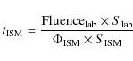
Appendix A:
Here we define the correlation between the radiation dose used in
the laboratory and the timescale in the interstellar clouds.
It is important to note that chemical modification of icy target
observed after ion irradiation depends, to a first approximation, on
the amount of energy that ions release into the target (dose in eV
molecule-1) and not on the type of ion.
Dose is defined as the product of ion flux (![]() ;
ions cm-2 s-1), stopping power (S; eV cm2 molecule-1) and time (t; s).
The product of ions flux and time is the fluence (ions cm-2).
Thus the time spent by grain mantles in the dense interstellar cloud to absorb a given dose is:
;
ions cm-2 s-1), stopping power (S; eV cm2 molecule-1) and time (t; s).
The product of ions flux and time is the fluence (ions cm-2).
Thus the time spent by grain mantles in the dense interstellar cloud to absorb a given dose is:
|
(A.1) |
where the flux
All Tables
Table 1: Details of experiments performed and discussed in this work.
Table 2: Thickness and density of the samples, stopping powers and the investigated dose ranges.
Table 3: List of integrated band strength (A) values used.
Table 4: Peak position of IR bands of unirradiated CO:SO2 ice as a mixture and layered sample.
Table 5: Peak position of the bands formed after irradiation of CO:SO2 as mixture and layered sample.
Table 6: Peak position of the IR bands of unirradiated CO:H2S ice a 10:1 mixture (mixture 1) and a 1:10 mixture (mixture 2) and of a layered film.
Table 7: Peak position of bands formed after irradiation of CO:H2S ice mixtures 10:1 (mixture 1) and 1:10 (mixture 2) and of a layered film.
Table 8: Abundances, relative to solid H2O and total H, of the S-bearing species detected in the icy grain mantles.
All Figures
|
|
Figure 1: IR transmittance spectra of CO:SO2 = 5:1 mixture as deposited at 16 K and after 200 keV H+ irradiation. |
| Open with DEXTER | |
| In the text | |
|
|
Figure 2: Normalized column density of CO and SO2 as a function of dose in CO:SO2 = 5:1 mixture ice at 16 K and in CO deposited on SO2 at 16 K. Points are connected for clarity. |
| Open with DEXTER | |
| In the text | |
|
|
Figure 3: The column densities of CO2, O3, and OCS and the band area of the SO3 doublet after 200 keV proton irradiation of CO:SO2 mixture or layered ices at 16 K as a function of dose. Data points are connected for clarity. |
| Open with DEXTER | |
| In the text | |
|
|
Figure 4: IR transmittance spectra of the CO:SO2 layered ice as deposited at 16 K and after irradiation with 200 keV H+. |
| Open with DEXTER | |
| In the text | |
|
|
Figure 5: IR transmittance spectra of CO:H2S 10:1 (mixture 1 - top panel) and 1:10 (mixture 2 - bottom panel) as deposited at 20 K and after irradiation with 200 keV H+. |
| Open with DEXTER | |
| In the text | |
|
|
Figure 6:
Normalized column density of CO, H2S, CO2, CS2, OCS, SO2 and the band area of H2S2 at 2486 cm-1 in CO:H2S mixtures 10:1 (mixture 1) and 1:10 (mixture 2) plotted as a function of dose. Column densities of CO, H2S and OCS, in CO:H2S
layered as a function of dose are also shown. The equivalence between
the doses used in laboratory and the time scale in cold dense IS clouds
(1 eV/16u |
| Open with DEXTER | |
| In the text | |
|
|
Figure 7: IR transmittance spectra of the CO:H2S layered ice as deposited at 20 K and after irradiation with 200 keV H+. |
| Open with DEXTER | |
| In the text | |
|
|
Figure 8:
Comparison between the fit obtained by the band of OCS observed in the CO:H2S = 10:1 mixture at the end of irradiation at 20 K and warmed at 60 K and the band at 4.9 |
| Open with DEXTER | |
| In the text | |
Copyright ESO 2010
Current usage metrics show cumulative count of Article Views (full-text article views including HTML views, PDF and ePub downloads, according to the available data) and Abstracts Views on Vision4Press platform.
Data correspond to usage on the plateform after 2015. The current usage metrics is available 48-96 hours after online publication and is updated daily on week days.
Initial download of the metrics may take a while.