| Issue |
A&A
Volume 509, January 2010
|
|
|---|---|---|
| Article Number | A49 | |
| Number of page(s) | 11 | |
| Section | Astronomical instrumentation | |
| DOI | https://doi.org/10.1051/0004-6361/200913019 | |
| Published online | 15 January 2010 | |
Compressive sensing for spectroscopy and polarimetry
A. Asensio Ramos1,2 - A. López Ariste3
1 - Instituto de Astrofísica de Canarias, 38205 La Laguna, Tenerife, Spain
2 -
Departamento de Astrofísica, Universidad de La Laguna, 38205 La Laguna, Tenerife, Spain
3 -
THEMIS, CNRS UPS 853, c/vía Láctea s/n, 38200 La Laguna,
Tenerife, Spain
Received 30 July 2009 / Accepted 24 September 2009
Abstract
We demonstrate, through numerical simulations with real data,
the feasibility of using compressive sensing techniques for the
acquisition of spectro-polarimetric data. This allows us to combine the
measurement and the compression process into one consistent framework.
Signals are recovered using a sparse reconstruction scheme from
projections of the signal of interest onto appropriately chosen
vectors, typically noise-like
vectors. The compressibility properties of spectral lines are analyzed
in detail. The results shown in this paper demonstrate that, thanks to
the compressibility properties of spectral lines, it is feasible to
reconstruct the signals using only a small fraction of the information
that is measured
nowadays. We investigate in depth the quality of the reconstruction as
a function of the amount of
data measured and the influence of noise. This change of paradigm also
allows us to define new instrumental
strategies and to propose modifications to existing instruments in
order to take advantage of compressive sensing techniques.
Key words: techniques: spectroscopic - techniques: polarimetric - methods: observational - magnetic fields
1 Introduction
Our present knowledge of the physical and magnetic properties of solar and stellar plasmas has benefited from the rapid development of spectro-polarimeters in the last decades. These instruments use dispersive elements for spectral analysis. Because visible/infrared detectors are only sensitive to the intensity of light, modulators are used to encode the polarimetric information on intensity variations. Since most detectors are nowadays two-dimensional, the recovery of two-dimensional spectro-polarimetric information is carried out using scanning techniques: spatial in the case of long-slit spectro-polarimeters and spectral in the case of Fabry-Perot-like spectro-polarimeters. According to the Nyquist-Shannon sampling theorem (Shannon & Weaver 1949; Nyquist 1928), the correct sampling of a band-limited signal should be done at a rate equal to twice the bandwidth. In other words, one should sample each resolution element (spectral and/or spatial) with at least two pixels in order to be ensure that all the frequencies in the bandwidth can be observed. This theorem has been applied for the last half century but it is only valid for band-limited signals.
During the last few years, the emerging theory of compressive sensing (CS; Candès et al. 2006b; Donoho 2006) has shown that this sampling is indeed too restrictive when some details of the signal structure are known in advance. An interesting point of the new CS paradigm is that, in many instances, natural signals have a structure that is known in advance. For instance, stellar oscillations can be represented by sinusoidal functions of different frequencies, images can be represented in a multiresolution analysis using wavelets, etc. The key point is that, typically, only a few elements of the basis set in which we develop the signal are necessary for an accurate description of the important physical information. The innovative character of CS is that this compressibility of the observed signals is inherently taken into account in the measurement step, and not only in the post-analysis, thus leading to efficient measurement protocols. Instead of measuring the full signal (wavelength variation of the Stokes profiles in our case), under the CS framework one measures a few linear projections of the signal along some vectors known in advance and reconstructs the signal solving a non-linear problem.
A review of the literature shows us that signals arising in natural phenomena are typically
compressible (see JPEG![]() compression and wavelet, curvelet or ridgelet decompositions of images, among
many others). Since this is also the case for astronomical data
(e.g., Polygiannakis et al. 2003; Mühlmann & Hanslmeier 1996; Belmon et al. 2002; Dollet et al. 2004; Bernas et al. 2004; Fligge & Solanki 1997), it has been suggested
that CS can be used to alleviate telemetry problems with space telescopes like
Herschel (Bobin et al. 2008) or Cassini (Belmon et al. 2002) and to improve
existing techniques for the reconstruction of radio interferometric data (Wiaux et al. 2009).
Several works demonstrate
that this is also true
in the field of polarimetry (López Ariste & Casini 2002; Socas-Navarro et al. 2001; Skumanich & López Ariste 2002; Casini et al. 2005).
Following this idea, Lites et al. (2002) analyzed the effectiveness of using JPEG
compression to reduce the amount of data that needs to be transferred through telemetry for
the Hinode space telescope. This option is currently in use in the mission (see Tsuneta et al. 2008).
All these results and those of the analysis we carry out in this paper
support the interest in investigating the appropriateness of employing
CS ideas to measure spectro-polarimetric signals, specifically for
space telescopes but also for ground-based telescopes. Through the use
of these techniques, we anticipate an enhanced performance in terms of
de-noising and data acquisition rates which eventually may have an
impact on the choice of detector technologies and data transfer.
compression and wavelet, curvelet or ridgelet decompositions of images, among
many others). Since this is also the case for astronomical data
(e.g., Polygiannakis et al. 2003; Mühlmann & Hanslmeier 1996; Belmon et al. 2002; Dollet et al. 2004; Bernas et al. 2004; Fligge & Solanki 1997), it has been suggested
that CS can be used to alleviate telemetry problems with space telescopes like
Herschel (Bobin et al. 2008) or Cassini (Belmon et al. 2002) and to improve
existing techniques for the reconstruction of radio interferometric data (Wiaux et al. 2009).
Several works demonstrate
that this is also true
in the field of polarimetry (López Ariste & Casini 2002; Socas-Navarro et al. 2001; Skumanich & López Ariste 2002; Casini et al. 2005).
Following this idea, Lites et al. (2002) analyzed the effectiveness of using JPEG
compression to reduce the amount of data that needs to be transferred through telemetry for
the Hinode space telescope. This option is currently in use in the mission (see Tsuneta et al. 2008).
All these results and those of the analysis we carry out in this paper
support the interest in investigating the appropriateness of employing
CS ideas to measure spectro-polarimetric signals, specifically for
space telescopes but also for ground-based telescopes. Through the use
of these techniques, we anticipate an enhanced performance in terms of
de-noising and data acquisition rates which eventually may have an
impact on the choice of detector technologies and data transfer.
The outline of the paper is the following. Section 2 gives a brief description of the CS paradigm, showing how signals can be recovered from a few linear projections and the properties that such projections need to fulfill. An analysis of the compressibility of spectro-polarimetric signals of interest is shown in Sect. 3. Section 4 presents recovery examples, with an analysis of the influence of noise. Section 5 shows novel instrumental strategies based on CS ideas, while the conclusions are presented in Sect. 6.
2 Compressive sensing
2.1 Theoretical considerations
Because of the innovative character of CS, we give a brief description of the most important points, while more mathematical details are discussed in Appendix A. For a more in-depth description, we refer the reader to recent references (e.g., Baraniuk 2007; Candès & Wakin 2008, and references therein).
The usage of compressive sensing techniques for the measurement of a signal ![]() represented as a vector of length M is based on the following two key ideas:
represented as a vector of length M is based on the following two key ideas:
- Instead of measuring the signal itself, one measures the scalar product of the signal with carefully selected vectors:
where is the vector of measurements of dimension N,
 is an
is an
 sensing matrix and
 is a vector of dimension N that characterizes the noise on the measurement process. Note that the previous
equation describes the most general linear multiplexing scheme in which the number of measurements M and the length of the signal N may differ. In the standard multiplexing case, the number of scalar products measured equals the dimension
of the signal (N=M). Consequently, it is possible to recover the vector
is a vector of dimension N that characterizes the noise on the measurement process. Note that the previous
equation describes the most general linear multiplexing scheme in which the number of measurements M and the length of the signal N may differ. In the standard multiplexing case, the number of scalar products measured equals the dimension
of the signal (N=M). Consequently, it is possible to recover the vector  provided
that
provided
that
 ,
so that the problem is not
ill-conditioned. In other words, one has to verify that every row of the
matrix is orthogonal with respect to every other row.
,
so that the problem is not
ill-conditioned. In other words, one has to verify that every row of the
matrix is orthogonal with respect to every other row.
- The second key ingredient of CS is the assumption that the
signal of interest is sparse in a certain basis set (or can be
efficiently compressed in this basis set). Any compressible
signal
![[*]](/icons/foot_motif.png) can be written, in general, as:
can be written, in general, as:
where is a K-sparse vector of size M and
 is the transpose of an
 transformation matrix associated with the basis set in which
the signal is sparse. For instance,
transformation matrix associated with the basis set in which
the signal is sparse. For instance,  can be the Fourier matrix if the signal
is the combination of a few sinusoidal components. Other
transformations of interest are the wavelet matrices or even empirical
transformation matrices like those found using principal component
analysis.
can be the Fourier matrix if the signal
is the combination of a few sinusoidal components. Other
transformations of interest are the wavelet matrices or even empirical
transformation matrices like those found using principal component
analysis.


with the hypothesis that
![\begin{figure}
\par\includegraphics[width=9cm]{13019f1.eps}
\end{figure}](/articles/aa/full_html/2010/01/aa13019-09/img18.png)
|
Figure 1: Test showing how compressive sensing works to detect a sparse signal. The upper panel shows a sparse signal made of four spikes of very short duration. The lower panel presents 24 measurements built as the scalar product of the signal with Gaussian random noise. The stars show the reconstructed signal, showing that perfect recovery is possible with only a very small fraction of the measurements. |
| Open with DEXTER | |
When the number of equations is less than the number of unknowns,
it is usual to solve Eq. (3) using least-squares methods that try to minimize the ![]() norm
norm![]() of the residual. This is usually accomplished using techniques based on the singular value decomposition (see, e.g., Press et al. 1986). However, such minimization is known
to return non-sparse results (e.g., Romberg 2008, and references therein). A more appropriate solution to Eq. (3)
is to look for the vector with the smallest
of the residual. This is usually accomplished using techniques based on the singular value decomposition (see, e.g., Press et al. 1986). However, such minimization is known
to return non-sparse results (e.g., Romberg 2008, and references therein). A more appropriate solution to Eq. (3)
is to look for the vector with the smallest ![]() pseudo-norm (the number of non-zero elements of the vector) that fulfills the equation (Candès et al. 2006b):
pseudo-norm (the number of non-zero elements of the vector) that fulfills the equation (Candès et al. 2006b):

where
is equivalent to that of Eq. (4). The advantage is that very efficient numerical methods exist for the solution of such problem (the one used in this paper is described in Appendix A).
Figure 1 shows a very simple example that summarizes the essence of compressive sensing. The upper panel presents a signal (solid line) that is 4-sparse in the basis of Dirac delta functions. Instead of measuring the full length of the signal, the lower panel of the figure shows a very small number of scalar products of the signal with a Gaussian random matrix. The stars present the reconstructed signal using only 24 such measurements. Since this is a noiseless example, perfect reconstruction is obtained.
2.2 Practical considerations
The CS framework offers several advantages over standard measurement paradigms. On the one hand, since one only measures linear combinations of the signals, the flux of information that any sensor has to deal with is usually much smaller (thanks to compression). This is probably of secondary interest for ground-based instruments since the infrastructure to cope with such large fluxes of data is available. However, this could be of interest for space-borne instruments, where the flux of data is limited by telemetry. As a sub-product of the simplification of the measurement, the reconstruction of the signal is much more time consuming, but can be done efficiently a-posteriori without affecting the measurement process. On the other hand, if appropriate sensing matrices are chosen, the measurement process can be considered universal and does not depend on the exact basis set in which the data is sparse. In other words, one first measures projections and this assures that the data can be reconstructed a-posteriori if the data is sparse in any (a priori unknown) basis set.
Ground-based instruments may draw advantages from the increased cadence at which data is acquired. An instrument measuring spatial and spectral information with a 2D detector is forced to scan one of the extra dimensions of the data space, either the spectra in filter instruments or one of the spatial dimensions in spectrograph instruments. The CS framework may diminish the number of measurements in the spectrum space thus shortening the time in which the 3D data cube is acquired by the instruments. Boosting data acquisition rates is always advantageous from both the point of view of a time evolving observational target (such as solar structures) or from the point of view of deformations or aberrations introduced by atmospheric turbulence (seeing).
![\begin{figure}
\par\mbox{\includegraphics[width=8.5cm]{13019f2a.eps}\includegrap...
...=8.5cm]{13019f2e.eps}\includegraphics[width=8.5cm]{13019f2f.eps} }\end{figure}](/articles/aa/full_html/2010/01/aa13019-09/img27.png)
|
Figure 2: Test showing the reconstruction of three widely known domains of the second solar spectrum: the top panels show a region around the Ba II D2, the middle panels a region around the Na I doublet at 5890 Å while the lower panel presents the region around the Sr I line at 4607 Å. Reconstruction using different wavelets and different thresholds are displayed. In each panel, the left panel presents how the reconstructed spectrum (red line) compares with the original spectrum using Daubechies-4, Daubechies-8, Coiflet-3 and Haar wavelets when 90% of the wavelet coefficients are set to zero. The right panels show the results when only 2% of the wavelet coefficients are retained. These results demonstrate that the structure of the lines is recovered with a small number of wavelet coefficients. Only in the case of the Sr I do we find spurious ripples (except in the Haar case) due to the loss of information. |
| Open with DEXTER | |
![\begin{figure}
\par\mbox{\includegraphics[width=8.7cm]{13019f3a.eps}\includegraphics[width=8.7cm]{13019f3b.eps} }\end{figure}](/articles/aa/full_html/2010/01/aa13019-09/img28.png)
|
Figure 3: Percentiles 68% (lines) and 95% (lines+symbols) of the differences between the true signal and the reconstructed signal when retaining a different percentage of the wavelet coefficients. The left panel corresponds to the data close to the Ba II D2 line, while the right panel shows the reconstruction of the Na I doublet. |
| Open with DEXTER | |
![\begin{figure}
\par\mbox{\includegraphics[width=8.8cm]{13019f4a.eps}\includegraphics[width=8.8cm]{13019f4b.eps} }\end{figure}](/articles/aa/full_html/2010/01/aa13019-09/img29.png)
|
Figure 4:
Percentile 68% (lines) and 95% (lines+symbols) of the differences
between the true signal and the reconstructed signal for a Hinode
observation. The left panel shows the case using a Daubechies-8 wavelet, the right panel presents the results using the PCA empirical basis set. The noise level in Stokes Q, U and V is close to
|
| Open with DEXTER | |
3 Compressibility of the signals
As reported in Sect. 2, any signal amenable to compressive sensing has to be sparse or compressible in some basis set. The purpose of this section is to test to what extent polarimetric signals are compressible (Asensio Ramos et al. 2007). We focus mainly on linear and circular polarization profiles, although our results can be extended to standard spectroscopic observations without effort. We present results for signals produced by scattering processes and for signals produced by the Zeeman effect in the presence of a magnetic field. Concerning the basis set in which the signals are sparse, we focus on the wavelet family for the case of scattering polarization and on the principal component analysis (PCA; Loève 1955) decomposition for the Zeeman case. These are just two possible candidates and we want to stress that it is advantageous to analyze each case in detail in order to find the basis set in which the signal is as sparse as possible.
3.1 Sparsity of the second solar spectrum
The wavelength variation of the fractional linear polarization Q/I measured very close to the solar limb is usually known as the second solar spectrum. Its name comes from the large wavelength variability, in some sense comparable to the standard Fraunhoffer intensity spectrum (see Gandorfer 2000,2002,2005). Examples of the variability are shown in Fig. 2, where many of the peaks detected correspond to specific spectral lines. Certain lines produce very conspicuous signals like the neutral sodium doublet shown in the middle panel of Fig. 2.
It is apparent that the spectrum of Q/I, in general, cannot be considered to be sparse in the wavelength domain because it is composed of broad peaks with a large wavelength variability. However, driven by the typical shape of the line profiles, we analyze the sparsity properties of the second solar spectrum when decomposed on the wavelet domain. To this end, we select standard wavelet mother functions that are widely used in other application (e.g., Jensen & la Cour-Harbo 2001): the Daubechies family, the Coiflet family and the Haar family. The discontinuous Haar family is appropriate for decomposing pixel-based data. The other families produce a smoother approximation to the data. It is left for the future to analyze the potential of other families, especially non-orthogonal redundant wavelets (e.g., Fligge & Solanki 1997; Starck et al. 1997) or Hermite functions (del Toro Iniesta & López Ariste 2003).
We carried out an experiment to characterize the compressibility of the second solar spectrum. We selected a large piece of the spectrum in which many small signals are present, together with a strong signal produced by the D2 line of Ba II. The spectrum is shown in black solid lines in Fig. 2. The full spectrum was wavelet-decomposed (the wavelet of choice is shown in each panel) and thresholded so that only a certain number of wavelet coefficients survive, while the rest of coefficients are set to zero. This is an efficient way of compressing the signal provided that the thresholding fundamentally cancels noise and leaves the signal unperturbed. The upper left panel of Fig. 2 shows what happens when only 10% of the wavelet coefficients are maintained, while the right panel indicates the behavior after setting 98% of the coefficients to zero. Since the zero coefficients are not necessary in the reconstruction, this thresholding leads to a large compression of the signal. The signal is then reconstructed using the inverse wavelet transform. We note that even in the case of only 2% of the coefficients, the important signals are recovered while the noisy part of the spectrum is largely reduced. It is apparent from the figure that the behavior is very similar for all the wavelet families we have tested, although the computing times are different, being larger for wavelets with a larger number of non-vanishing moments (e.g., Jensen & la Cour-Harbo 2001). This can be an issue that should be taken into account depending on the balance between the desired smoothness of the reconstruction and the computing time.
Other examples are shown in the middle and lower panels of Fig. 2, for the case of the Na I doublet at 5890 Å and the Sr I line at 4607 Å, respectively. The first one presents a case in which low-frequency (the large scale quantum interference between the two lines of the doublet) and high-frequency information (the large variability of the profiles close to the core of the line) coexist. This poses an interesting problem to any compression method because it has to retain low and high frequencies simultaneously. Apparently, the wavelet compression does a good job on this multiplet and all important details can be retrieved even with only 2% of the coefficients. The lower panels of Fig. 2 show the case of the Sr I line at 4607 Å, which is a very strong signal embedded in a quasi-flat continuum. In this case, reconstructing only with 2% of the coefficients gives a poor representation of the true underlying signal. Some ripples appear when using Daubechies and Coiflet wavelets on the quasi-continuum, although the amplitude of the signal is still correctly recovered. The reconstruction with the Haar wavelet gives a very good representation of the Sr I line but the depolarizations in the red wing of the line and at 4606.3 Å are not correctly recovered. The reconstruction with 10% of the coefficients is almost perfect.
We have measured the quality of the reconstruction
using the 68% and 95 % percentiles of the difference between the
original and the reconstructed signal. The value of these quantities
versus the percentage of remaining non-zero coefficients is shown in
Fig. 3. The left panel has been obtained with the data from the Ba II D2line, while the right panel is associated with the Na I data.
We have verified that the distribution of differences is close to normal except in
the cases in which the reconstruction is done with too few coefficients. Therefore, the 68% and 95% percentiles
are close to the standard deviation and twice the standard deviation, respectively. The lines without symbols
present the 68% percentile, showing that differences are in both cases below 10-2 when retaining
just 10% of the profiles. For Q/I signals that are on average at the level of ![]() 0.1, we find that relative
errors are typically below 10-3. The 95% percentile gives relative errors slightly above 10-3 for
these cases. The results tend to indicate that differences among wavelet families are relatively small.
0.1, we find that relative
errors are typically below 10-3. The 95% percentile gives relative errors slightly above 10-3 for
these cases. The results tend to indicate that differences among wavelet families are relatively small.
3.2 Sparsity of Zeeman signals
In the presence of a sufficiently strong magnetic field, the Zeeman effect usually controls the emergent observed polarization. In order to test for the compressibility properties in the Zeeman-dominated case, we use a dataset obtained with the Solar Optical Telescope/Spectro-Polarimeter SOT/SP (Lites et al. 2001) aboard Hinode (Kosugi et al. 2007). The properties of this dataset are typical of what one should encounter in the future if the CS techniques that we propose here are applied to future space missions. In this case, we test two different basis set for compressibility in Fig. 4. The first is the universal Daubechies-8 wavelet (left panel). The results we show are not very sensitive to the specific chosen wavelet and are representative of the general behavior. The second is the empirical basis set obtained using the PCA decomposition (right panel).
![\begin{figure}
\par\mbox{\includegraphics[width=8.8cm]{13019f5a.eps}\includegrap...
...5c.eps}\includegraphics[width=8.8cm]{13019f5d.eps} }\vspace*{5mm}
\end{figure}](/articles/aa/full_html/2010/01/aa13019-09/img31.png)
|
Figure 5: Examples of CS reconstructions of four different polarization signals. The left panels present the results for signals produced by scattering polarization when observed close to the limb. Reconstruction is done using Daubechies-8 wavelets. The right panels show reconstructions of Zeeman signals observed with Hinode. Reconstruction is done using a universal PCA basis. Additionally, we show the difference on the reconstruction using two different sensing matrices: a Gaussian matrix with zero mean and inverse variance equal to the sparsity of the signal and a sparse binary sensing matrix with 10 non-zero elements per measurement. In general, we find a better behavior for the sparse binary matrix than for the random full matrix. |
| Open with DEXTER | |
The results, that present the 68% and 95% percentiles of the distribution of the difference between the exact and the reconstructed profiles, indicate clearly that signals are again compressible. The best results are, obviously, obtained with the PCA basis set, because the eigenvectors are empirically constructed to maximize the sparsity of the signal (only a few eigenvectors are necessary to reconstruct the signal without noise).
The main problem with the PCA basis set is that it is obtained empirically. Consequently, strictly speaking, one is not able to use the PCA basis set in a CS framework because a-priori the basis set is not known. However, according to Skumanich & López Ariste (2002), some universality properties of the PCA eigenvectors can be demonstrated when many profiles are included in a database. For this reason, we have tested that profiles observed with Hinode can be well compressed with the eigenvectors recovered from a completely different dataset. The reason is that the same physical effects control the signals in both datasets. This opens up the possibility of using some kind of universal PCA basis when compressing Zeeman-dominated data. This basis set will likely contain details of the spectral lines that are present in the majority of the observed profiles and that can be poorly recovered with fixed basis sets like wavelets.
4 Signal recovery
4.1 Examples
Since we have demonstrated that the polarimetric signals are compressible, the CS framework can be used to measure such signals. We give here a few examples using different sensing matrices. The first ones are shown in the left panel of Fig. 5. We present the reconstruction of the Na I and Sr I signals analyzed in Sect. 3 with two different sensing matrices: (i) a Gaussian matrix with elements extracted from the N(0,1/K) distribution (Candès et al. 2006b), with K being the sparsity of the signal; and (ii) a binary sparse sensing matrix with only 10 non-zero elements per measurement (Berinde & Indyk 2008). Obviously, the binary sparse matrix has two advantages over the Gaussian matrix. First, the number of non-zero elements is very small as compared to the size of the matrix and efficient sparse storage and computational methods can be used (e.g., Press et al. 1986). In our case, the sparse matrix contains less than 2% of the elements different from zero. Second, the binary matrix is easier to implement on hardware using, for instance, micro-mirrors. Only 5% of the elements of the solution vector are allowed to be non-zero for the case of Na I and 10% for the case of Sr I, according to the results presented in Fig. 2. The number of measurements used is 6 K for the Sr I line and 8 K for the Na I doublet, roughly in accordance with Eq. (A.6), while the reconstruction is done using the Daubechies-8 wavelet. The results show that a good recovery is possible in the two cases, with the advantage that, since sparsity is inherent to the reconstruction, noise is largely reduced in the reconstruction. In order to show how the technique behaves with the number of measurements, we show in Fig. 6 the standard deviation of the difference between the reconstructed and original signal versus the number of measurements (normalized to the sparsity of the vector). The horizontal lines indicate an estimation of the noise level in the observations obtained as the standard deviation of a portion of the continuum. Note that when the number of measurements is not large enough, the reconstruction does not work. However, as soon as condition (A.6) is fulfilled, reconstruction works properly.
Other examples are shown on the right panel of Fig. 5, the Stokes Vprofiles picked at two positions of an observation carried out with Hinode on February 27, 2007. The Fe I doublet at 630 nm with amplitudes typical of active regions (upper panel) and quiet Sun (lower panel) are shown in black lines. The reconstructed signals using the same sensing matrices as above are shown in red and blue. The universal PCA basis is used and only 11 of such eigenvectors are used, roughly 10% of the full basis set. The number of measurements is 6 K, in accordance with Eq. (A.6). A good recovery is possible even for profiles whose amplitude is close to the noise level. The prior information encoded in the sparse reconstruction produces that noise is slightly reduced with respect to the original profile. This is similar to what one would find after carrying out a PCA filtering of the data, but the filtering is encoded inside the measurement technique (e.g., Martínez González et al. 2008b). The fundamental reason for this is that, while true signals produce sparse signatures, noise destroys the sparsity to some degree. Since the reconstruction is done enhancing sparsity, it is not possible to recover noise and a filtering is carried out as a side effect of the reconstruction.
![\begin{figure}
\par\includegraphics[width=9cm]{13019f6.eps}
\end{figure}](/articles/aa/full_html/2010/01/aa13019-09/img32.png)
|
Figure 6: Standard deviation of the difference between the recovery and the original signal for different numbers of measurements. The reconstruction is done using the sparse binary matrix and the Daubechies-8 wavelet. |
| Open with DEXTER | |
4.2 Sensitivity to noise
To test the influence of noise on our ability to recover the spectrum
from the linear combinations
given by the sensing matrix, we analyze a synthetic case. We have
chosen the spectral line at 6302 Å for its widespread use. A very
simplistic Stokes I profile is built using a Voigt function tweaking the
width and depth to fit the average profile of the solar atlas (Wallace et al. 1998).
The Stokes V profile emerging from a magnetized atmosphere is built under the weak-field approximation, in which
it is proportional to the wavelength derivative of Stokes I (e.g., Landi Degl'Innocenti & Landolfi 2004). We used
a magnetic flux density of 1 Mx/cm-2, resulting in an amplitude
of
![]() in units of the continuum intensity. The small value of the magnetic flux density is used intentionally so that the
observation is close to the detection limit of present spectro-polarimeters with relatively short exposure
times. We simulate observations with noise added and we use a Gaussian random sensing matrix with zero
mean and inverse variance equal to the assumed sparsity. We carry out experiments, shown in
Fig. 7,
using Daubechies-8 wavelets assuming that only 12 elements of the
recovered vector are non-zero (left panel) and a universal PCA basis
set assuming that the sparsity
of the vector is 5 (right panel). The PCA basis is obtained from a
dataset observed with Hinode. The number of measurements is set to six
times the sparsity level in each case. The solid line in each plot
indicates the standard deviation of the difference between the exact
profile and the reconstructed one for each value of the noise level.
The dashed line is the same quantity but calculated only for the noise.
This curve is used to give an idea of the de-noising abilities of the
decomposition on a wavelet/PCA basis. When the signal-to-noise ratio
(SNR) is very poor, in both experiments we see a reduction of almost an
order of magnitude in the noise, showing that the signal is well below
the noise level. Only when the SNR approaches
in units of the continuum intensity. The small value of the magnetic flux density is used intentionally so that the
observation is close to the detection limit of present spectro-polarimeters with relatively short exposure
times. We simulate observations with noise added and we use a Gaussian random sensing matrix with zero
mean and inverse variance equal to the assumed sparsity. We carry out experiments, shown in
Fig. 7,
using Daubechies-8 wavelets assuming that only 12 elements of the
recovered vector are non-zero (left panel) and a universal PCA basis
set assuming that the sparsity
of the vector is 5 (right panel). The PCA basis is obtained from a
dataset observed with Hinode. The number of measurements is set to six
times the sparsity level in each case. The solid line in each plot
indicates the standard deviation of the difference between the exact
profile and the reconstructed one for each value of the noise level.
The dashed line is the same quantity but calculated only for the noise.
This curve is used to give an idea of the de-noising abilities of the
decomposition on a wavelet/PCA basis. When the signal-to-noise ratio
(SNR) is very poor, in both experiments we see a reduction of almost an
order of magnitude in the noise, showing that the signal is well below
the noise level. Only when the SNR approaches ![]() 0.4 do we see that the CS detects signal and gives a much better behavior than just the
direct measure of the profile using standard techniques. The reason lies in the fact that sparsity
is promoting the detection of signals, contrary to the detection of noise. Noise is not sparse
in any of the basis sets used and the reconstruction is made assuming sparsity in the solution. This
is important information that we are including as a prior in the CS recovery, something that is not
done in standard measurements.
0.4 do we see that the CS detects signal and gives a much better behavior than just the
direct measure of the profile using standard techniques. The reason lies in the fact that sparsity
is promoting the detection of signals, contrary to the detection of noise. Noise is not sparse
in any of the basis sets used and the reconstruction is made assuming sparsity in the solution. This
is important information that we are including as a prior in the CS recovery, something that is not
done in standard measurements.
![\begin{figure}
\par\mbox{\includegraphics[width=8.8cm]{13019f7a.eps}\includegraphics[width=8.8cm]{13019f7b.eps} }\end{figure}](/articles/aa/full_html/2010/01/aa13019-09/img33.png)
|
Figure 7:
Noise level of the CS reconstructed signal versus the noise level of each individual measurement. The left panel shows the reconstruction with a wavelet basis set while the right panel
has been obtained using a universal PCA basis set. The sparsity in the
wavelet case is assumed to be 12, while this number is reduced to
5 for the PCA case. The dashed line shows the reconstruction error
when only noise is taken into account. The dotted line is the diagonal,
the expected noise level if a standard spectrograph is used. For
comparison, the maximum amplitude of the signal is
|
| Open with DEXTER | |
4.3 CS with polarimetric modulation
Since existing instruments are not directly sensitive to polarization
in the optical and infrared spectral domains, it is customary to use
modulation schemes to measure the Stokes parameters.
In some sense, modulation is another form of multiplexing which is
carried out using retarders and polarizers. The monochromatic Stokes
vector entering the telescope ![]() is modulated
is modulated
![]() times to generate intensities that are linear combinations of the Stokes parameters of
times to generate intensities that are linear combinations of the Stokes parameters of ![]() :
:

|
(6) |
where each row of the
The obvious question is whether it is possible to apply CS to compress
the wavelength information while still carrying out the modulation to
detect the four Stokes parameters. The answer is that it is possible
since both multiplexing operations ``act'' on different spaces:
polarimetric modulation
applies to monochromatic Stokes parameters and the sensing matrix of CS
applies to the wavelength variation of a single Stokes parameter.
Therefore, under the assumption that the polarimetric modulation is
achromatic over the observed spectral range, their effect can be
interchanged and one ends up solving four problems of the kind:
where
4.4 Fringes and other spurious signals
Among others, non-polarized and polarized fringes are undesirable contaminations present in many spectro-polarimetric observations (e.g., Semel 2003). Observations are partially cleaned of these fringes using flat-fielding techniques. The remaining fringes are filtered out at the end of the reduction process with the disadvantage of having a large subjective component. Under the compressive sensing scheme, these spurious signals are measured together with the real signal. In the reconstruction we try to avoid introducing them in the final result, be it by rejecting or reconstructing them together with the true signal. Obviously, the ideal situation is to employ a fringe-free spectro-polarimeter to obtain a better reconstruction. We defer the deep investigation of this issue to a later study. However, preliminary experiments indicate that the reconstruction can efficiently reduce the amplitude of periodic fringes if the basis set used is not able to reproduce them. The drawback is that the ensuing reconstruction is less accurate than in the absence of fringes. Such a situation arises when applying a PCA basis set that is able to efficiently describe the spectro-polarimetric signals but not the periodic fringes. Another possibility of investigation is to assume that the fringes are sparse in the Fourier domain, carrying out the reconstruction merging the Fourier basis set and the basis set for the signal.
5 Applications
5.1 Efficient spectro-imagers
Recent interest in Hadamard techniques for spectro-polarimetry (see Harwit & Sloane 1979, for more details) can greatly benefit from CS techniques. Hadamard techniques allow us to condensate spectral information inside single detector pixels through multiplexing. Before going into the use of these techniques in the framework of CS, it is advisable to describe these Hadamard techniques in spectro-polarimetry and the advantages they bring through two illustrative examples. In traditional spectroscopy, a certain number of pixels (often a full dimension of a detector array) are dedicated to measure intensities at different wavelengths for the same point in an image. In Hadamard techniques, this is substituted by a temporal modulation over the Hadamard cyclic mask in a single detector pixel. Such an exchange has two interesting applications: in long-slit spectroscopy, the spectrum can be multiplexed in a single pixel and instead of using a 2-dimensional detector array one can use a one dimensional array with increased acquisition cadences that allow us to freeze the seeing during the modulation cycle of polarimetry with the resulting improvement on polarimetric sensitivity (see, e.g., ZIMPOL; Povel 2001).
In double-pass subtractive spectroscopy (Mein 2002), the resulting image has been filtered by a narrow spectral slit that selects a single wavelength per pixel. Due to the dispersion of the first pass over the diffraction grating, the selected wavelength changes as one moves over the spatial image. To reconstruct the full 3D data cube with both spatial dimensions and spectral covering, every pixel has to be scanned over a range of wavelengths. Through the use of Hadamard cyclic matrices one can have several wavelengths sampled simultaneously in every pixel. As a result the temporal coherence of the recovered spectra is increased as several wavelengths over the spectral domain are detected simultaneously. Also, as a side effect, the raw images do not show any evident spectral features, which makes them more suitable for image reconstruction techniques
Such applications of Hadamard techniques to spectro-polarimetry are however hindered by the known fact that, in the presence of a multiplicative noise such as photonic noise, the Hadamard transformation results in a reduction of SNRs with respect to the case of equivalent exposures without multiplexing (Harwit & Sloane 1979). The reduction in the SNR can be limited with the use of appropriate binary masks (Wuttig 2005), although it is never too large for the usual cases in solar spectro-polarimetry.
Compressive sensing can help mitigate the problem. Since the Hadamard
technique is applied to the spectral information, one can make use of
the fact that there is prior information about the spectrum
to be measured and that, as a consequence, the space of spectral
profiles (with polarization included) is sparse, as demonstrated in the
previous sections of this work. The use of the CS techniques
illustrated above allows the recovery of the full spectral information
with just a few spectral measurements. In the terminology of Hadamard
techniques, this translates into the fact that not all the data
acquisitions attached to the cyclic Hadamard masks are required for the
recovery of the spectrum. If traditionally a Hadamard mask of
dimension N would require N cyclic measurements to solve the multiplexing linear system, CS techniques may be used to solve the system with just MK acquisitions,
where ![]() is the sparsity of the signal (perhaps
is the sparsity of the signal (perhaps
![]() at most) and M > 1 is a small number. If each exposure lasts for
at most) and M > 1 is a small number. If each exposure lasts for
![]() ,
the reduction in the required time for spectral information
retrieval (from
,
the reduction in the required time for spectral information
retrieval (from
![]() to
to
![]() )
can then be used, not only to accelerate the full process of measurement, but also to repeat the same measurement N/(MK) times and add them to gain a factor
)
can then be used, not only to accelerate the full process of measurement, but also to repeat the same measurement N/(MK) times and add them to gain a factor
![]() in signal to noise ratio. From the tests of previous sections we can conclude that a figure of K = 0.1 N is sufficient for the precisions required. With a factor
in signal to noise ratio. From the tests of previous sections we can conclude that a figure of K = 0.1 N is sufficient for the precisions required. With a factor ![]() ,
the repetition of the measurements with a reduced Hadamard cycle can be used to gain roughly a factor
,
the repetition of the measurements with a reduced Hadamard cycle can be used to gain roughly a factor
![]() in SNR. Such a factor would largely compensate the loss of SNR inherent
to the use of the Hadamard techniques with multiplicative photon noise.
We conclude that the use of compressive sensing is strongly recommended
for a successful application of Hadamard techniques to
spectro-polarimetry.
in SNR. Such a factor would largely compensate the loss of SNR inherent
to the use of the Hadamard techniques with multiplicative photon noise.
We conclude that the use of compressive sensing is strongly recommended
for a successful application of Hadamard techniques to
spectro-polarimetry.
![\begin{figure}
\par\includegraphics[width=9cm]{13019f8.eps}
\end{figure}](/articles/aa/full_html/2010/01/aa13019-09/img50.png)
|
Figure 8: Example showing how reliable reconstructions of high-resolution signals can be obtained from rebinned data, provided that the signal is considered to be compressible. The upper panel shows the original (black) and reconstructed profiles using 1/2 (red) and 1/4 (blue) of the original resolution. The data is reconstructed with 5 PCA eigenvectors of a universal basis set. The lower panel shows the measurements from which the reconstructions are obtained. The original signal is shown in black, while red and blue lines show measurements rebinned to 1/2 and 1/4 of the original resolution. |
| Open with DEXTER | |
5.2 Sub-Nyquist spectrograph
When prior information about the expected signals is available
it is possible to imagine a spectrograph able to measure the wavelength
variation of the Stokes parameters using resolution elements (pixels in
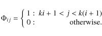
the camera) larger than the spectral sampling. In such a case, if one
measures with a camera containing
![]() pixels, each one integrating k spectral sampling steps, the sensing matrix of size
pixels, each one integrating k spectral sampling steps, the sensing matrix of size
![]() can be written:
can be written:
|
(8) |
This sensing matrix is probably not very efficient for reducing to the optimal value the number of CS measurements but it suffices for our aims, since we are typically interested in cases where k is not very large. An example of this is shown in Fig. 8. A Stokes V profile observed with Hinode, shown in black lines in both panels, is rebinned to 1/2 and 1/4 the original resolution by adding two/four consecutive pixels together. The corresponding measurements are shown in the lower panel with red and blue lines, respectively. Using five PCA eigenvectors of the universal set discussed in Sect. 3.2, the signals are reconstructed solving the
We point out that, if the signal is known to be sparse in the Fourier basis, one could consider that the Nyquist-Shannon theorem should be applied to the frequency support where the signal is defined in the frequency domain. This is the case of signals for which the power associated with frequencies above a certain threshold is associated with noise. In such a case, one can use this new threshold, using the Nyquist-Shannon sampling theorem, to estimate the number of pixels per resolution element. Reconstruction should be done using the appropriate prior information. We have verified, although not shown here, that good reconstructions can be obtained using 1/2 and 1/4 of the original information by employing the Fourier basis set and forcing the signal in the Fourier domain to be sparse. This has the advantage over PCA eigenvectors that they are fully universal.
5.3 Hadamard-PCA magnetometer
The combination of CS ideas and standard PCA techniques can be
applied to develop an efficient magnetometer. To this end, let us
assume that the Stokes V profile is well represented using the first PCA eigenvector
![]() obtained empirically from a set of previous observations:
obtained empirically from a set of previous observations:
This equation assumes, therefore, that the observed Stokes profiles are 1-sparse in the PCA basis set, so that one can recover the signal, according to the CS theory, using of the order of 4-6 measurements. Using a sensing matrix
|
(10) |
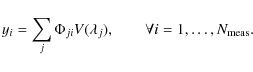
If the sparsity constraint is used, the proportionality constant A can be obtained from the observations with a linear fit:

|
(11) |
where
If enough measurements are taken, it is possible to include more eigenvectors in the decomposition of Eq. (9) and obtain information about the projection along them from the observations. If Stokes I is decomposed, continuum images and velocities can be inferred from the first and second eigenvectors, respectively. Likewise, if Stokes V is used, magnetic flux and magnetic velocities can be inferred.
![\begin{figure}
\par\includegraphics[width=9cm]{13019f9.eps}
\end{figure}](/articles/aa/full_html/2010/01/aa13019-09/img61.png)
|
Figure 9: Comparison between the measured Stokes V amplitude and the one measured using CS techniques with a Hadamard sensing matrix. The black dots show the comparison when only one measurement is made, while the red dots present the results using 8 measurements. |
| Open with DEXTER | |
6 Conclusions
This paper demonstrates the feasibility of applying compressive sensing techniques to measure the wavelength variation of the Stokes parameters observed in stellar atmospheres. We have shown that spectro-polarimetric signals are, in general, compressible on universal basis sets. However, in general, it is more advantageous to use empirical basis sets like that obtained from principal component analysis because data can be more efficiently reproduced on such a basis. We stress that the results presented in this paper are extensible to standard spectroscopic observations and not only to linear and circular polarization profiles, so that any day-time and night-time spectrograph can take advantage of these techniques.
According to our results, it is possible to measure Stokes parameters using less than a half of the measurements one would need when strictly applying the Nyquist-Shannon sampling theorem. Compressive sensing leads to several interesting effects. Since fewer measurements are made, an inherent reduction in the exposure time is present. Such a reduction can be used to do more measurements in the same total time, thus allowing less noisy observations. The a-priori information encoded in the sparsity condition results in the fact that the reconstructed signal is much less noisy than one would expect. The reason is that filtering is applied simultaneously while measuring. For instance, several of the examples shown in this paper produce signals that are automatically filtered with the principal component analysis applied by Martínez González et al. (2008a,b).
We have proposed potential applications of CS to the field of spectro-polarimetry, testing them numerically on real data. Some of these techniques can be straightforwardly applied to existing instruments, while other proposals need more profound modifications. The future of observational spectro-polarimetry, at least in solar physics, has to be rooted in the development of two-dimensional spectro-polarimeters. Since detectors are only two-dimensional at the moment, scanning schemes have to be used. We consider that double-pass subtractive spectroscopy constitutes a very appealing technique for two-dimensional spectro-polarimetry if combined with multiplexing techniques using Hadamard masks. Compressive sensing will help significantly reduce the total exposure time, thus allowing an increase in the final SNR for a fixed integration time.
Because of the natural physical interpretation of projections of the observed Stokes profiles along PCA eigenvectors (Skumanich & López Ariste 2002), it would be desirable to directly measure such projections. Using compressive sensing techniques, we have proposed a technique that, thanks to Hadamard masks, is able to retrieve such projections from a universal multiplexing. The advantage is that this multiplexing is binary and easy to build.
Finally, we analyze the plausibility of a spectro-polarimeter that does not fulfill the Nyquist-Shannon sampling theorem. Some a-priori information about the expected signals is available and compressive sensing techniques can take full advantage of this information to recover the signals from a reduced set of measurements. We show with an example that it is possible to reconstruct Stokes profiles using the information obtained from adding the signal in consecutive pixels. This can be understood as a super-resolution scheme in which one knows the basis set in which the high-resolution signal can be efficiently developed.
AcknowledgementsWe thank Rafael Manso Sainz and María Jesús Martínez González for illuminating discussions and carefully reading the manuscript. Financial support by the Spanish Ministry of Science and Innovation through project AYA2007-63881 is gratefully acknowledged.
Appendix A: Compressive sensing
As noted in the main text, the multiplexing scheme for a sparse signal reads:

|
(A.1) |
with the condition that
where
is equivalent to that of Eq. (A.2). The RIP condition is a sufficient condition and it is often too restrictive. The advantage of the last problem is that it can be easily solved using linear programming techniques.
Intuitively, the RIP condition states that the action of the
![]() operator on the sparse vector
operator on the sparse vector ![]() does not excessively modify its
does not excessively modify its ![]() norm. Mathematically:
norm. Mathematically:
|
(A.4) |
for all K-sparse vectors
In spite of the mathematical importance of the RIP condition, it is
more intuitive to think in terms of coherence between the sensing
matrix and the transformation matrix. In general, for a sensing matrix
to be considered good, it should be as incoherent as possible
with the transformation matrix. Every row of the sensing matrix should
be able to obtain as much
information as possible from the sparse vector ![]() in order to facilitate its
reconstruction with as few measurements as possible. This is achieved when the sensing
matrix and the transformation matrix are as incoherent as possible. The coherence
between the two matrices is defined as (Candès & Romberg 2007):
in order to facilitate its
reconstruction with as few measurements as possible. This is achieved when the sensing
matrix and the transformation matrix are as incoherent as possible. The coherence
between the two matrices is defined as (Candès & Romberg 2007):
|
(A.5) |
where
where C is a constant of order 1. According to this equation, if one is able to find sensing matrices with small coherence with respect to the basis set of interest, one should be able to recover the sparse signal using a number of measurements that is proportional to
A.1 Recovery algorithm
For the recovery problem in our experiments, different methods have
been developed during the last few years. After testing several methods, we found that the recent algorithm presented by Blumensath & Davies (2008)
is very efficient in terms of computing time and shows state of the art
performance. The method uses the simple iterative procedure:
![\begin{displaymath}{\vec x}^{n+1} = {\rm H}_s \left[ {\vec x}^{n} + \mu {\vec W}...
...} - \mathbf{\Phi} {\vec W}^{\rm T} {\vec x}^n \right) \right],
\end{displaymath}](/articles/aa/full_html/2010/01/aa13019-09/img71.png)
where H s(t) is a non-linear thresholding operator that leaves as non-zero the s elements of the vector t with the largest absolute value, setting to zero the rest of elements. The method is guaranteed to be stable thanks to the re-scaling quantity
References
- Asensio Ramos, A., Socas-Navarro, H., López Ariste, A., et al. 2007, ApJ, 660, 1690 [NASA ADS] [CrossRef] [Google Scholar]
- Baraniuk, R. 2007, IEEE Signal Processing Magazine, 24, 118 [Google Scholar]
- Belmon, L., Benoit-Cattin, H., Baskurt, A., et al. 2002, A&A, 386, 1143 [Google Scholar]
- Berinde, R., & Indyk, P. 2008, Computer Science and Artificial Intelligence Laboratory Technical Report, MIT-CSAIL-TR-2008-001 [Google Scholar]
- Bernas, M., Páta, P., Weinlich, J., Hudec, R., & Castro Tirado, A. 2004, in 5th INTEGRAL Workshop on the INTEGRAL Universe, ed. V. Schoenfelder, G. Lichti, & C. Winkler, ESA SP, 552, 829 [Google Scholar]
- Blumensath, M. E., & Davies, M. E. 2008, The Journal of Fourier Analysis and Applications, 14, 629 [CrossRef] [Google Scholar]
- Bobin, J., Starck, J.-L., & Ottensamer, R. 2008, IEEE Journal of Selected Topics in Signal Processing, 2(5), 718 [Google Scholar]
- Candès, E., & Romberg, J. 2007, Inverse Problem, 3, 969 [Google Scholar]
- Candès, E., Romberg, J., & Tao, T. 2006a, IEEE Transactions on Information Theory, 52, 489 [CrossRef] [MathSciNet] [Google Scholar]
- Candès, E., Romberg, J., & Tao, T. 2006b, Comm. Pure Appl. Math., 59, 1207 [CrossRef] [Google Scholar]
- Candès, E. J., & Wakin, M. B. 2008, IEEE Signal Processing Magazine, 25, 21 [Google Scholar]
- Casini, R., Bevilacqua, R., & López Ariste, A. 2005, ApJ, 622, 1265 [NASA ADS] [CrossRef] [Google Scholar]
- Dollet, C., Bijaoui, A., & Mignard, F. 2004, A&A, 426, 729 [Google Scholar]
- Donoho, D. 2006, IEEE Trans. on Information Theory, 52, 1289 [CrossRef] [Google Scholar]
- Fligge, M., & Solanki, S. K. 1997, A&AS, 124, 579 [Google Scholar]
- Gandorfer, A. 2000, The Second Solar Spectrum, I: 4625 Å to 6995 Å (Zurich: vdf) [Google Scholar]
- Gandorfer, A. 2002, The Second Solar Spectrum, II: 3910 Å to 4630 Å (Zurich: vdf) [Google Scholar]
- Gandorfer, A. 2005, The Second Solar Spectrum, III: 3160 Å to 3915 Å (Zurich: vdf) [Google Scholar]
- Harwit, M., & Sloane, N. J. A. 1979, Hadamard Transform Optics (London: Academic Press) [Google Scholar]
- Jensen, A., & la Cour-Harbo, A. 2001, Ripples in Mathematics: The Discrete Wavelet Transform (Springer Verlag) [Google Scholar]
- Kosugi, T., Matsuzaki, K., Sakao, T., et al. 2007, Sol. Phys., 243, 3 [NASA ADS] [CrossRef] [Google Scholar]
- Landi Degl'Innocenti, E., & Landolfi, M. 2004, Polarization in Spectral Lines (Kluwer Academic Publishers) [Google Scholar]
- Lites, B., Shine, R. A., López Ariste, A., et al. 2002, AGU Fall Meeting Abstracts, A471 [Google Scholar]
- Lites, B. W., Elmore, D. F., Streander, K. V., et al. 2001, in UV/EUV and Visible Space Instrumentation for Astronomy and Solar Physics, ed. O. H. Siegmund, S. Fineschi, & M. A. Gummin, Proc. SPIE, 4498, 73 [Google Scholar]
- Loève, M. M. 1955, Probability Theory (Princeton: Van Nostrand Company) [Google Scholar]
- López Ariste, A., & Casini, R. 2002, ApJ, 575, 529 [NASA ADS] [CrossRef] [Google Scholar]
- Martínez González, M. J., Asensio Ramos, A., Carroll, T. A., et al. 2008a, A&A, 486, 637 [Google Scholar]
- Martínez González, M. J., Collados, M., Ruiz Cobo, B., et al. 2008b, A&A, 477, 953 [Google Scholar]
- Mein, P. 2002, A&A, 381, 271 [Google Scholar]
- Mühlmann, W., & Hanslmeier, A. 1996, Sol. Phys., 166, 445 [NASA ADS] [CrossRef] [Google Scholar]
- Nyquist, H. 1928, Trans. AIEE, 617 [Google Scholar]
- Polygiannakis, J., Preka-Papadema, P., & Moussas, X. 2003, MNRAS, 343, 725 [NASA ADS] [CrossRef] [Google Scholar]
- Povel, H. P. 2001, in Magnetic Fields across the Hertzsprung-Russel Diagram, ed. G. Mathys, S. K. Solanki, & D. T. Wickramasinghe, ASP Conf. Ser., 248, 543 [Google Scholar]
- Press, W. H., Teukolsky, S. A., Vetterling, W. T., et al. 1986, Numerical Recipes (Cambridge: Cambridge University Press) [Google Scholar]
- Romberg, J. 2008, IEEE Signal Processing Magazine, 25, 14 [Google Scholar]
- Semel, M. 2003, A&A, 401, 1 [Google Scholar]
- Shannon, C. A., & Weaver, W. 1949, The Mathematical Theory of Communication (University of Illinois Press) [Google Scholar]
- Skumanich, A., & López Ariste, A. 2002, ApJ, 570, 379 [NASA ADS] [CrossRef] [Google Scholar]
- Socas-Navarro, H., López Ariste, A., & Lites, B. W. 2001, ApJ, 553, 949 [NASA ADS] [CrossRef] [Google Scholar]
- Starck, J.-L., Siebenmorgen, R., & Gredel, R. 1997, ApJ, 482, 1011 [NASA ADS] [CrossRef] [Google Scholar]
- del Toro Iniesta, J. C., & Collados, M. 2000, Appl. Opt., 39, 1637 [NASA ADS] [CrossRef] [PubMed] [Google Scholar]
- del Toro Iniesta, J. C., & López Ariste, A. 2003, A&A, 412, 875 [Google Scholar]
- Tsuneta, S., Ichimoto, K., Katsukawa, Y., et al. 2008, Sol. Phys., 249, 167 [NASA ADS] [CrossRef] [Google Scholar]
- Wallace, L., Hinkle, K., & Livingston, W. 1998, An atlas of the spectrum of the solar photosphere from 13 500 to 28 000 cm-1 (3570 to 7405 A), ed. L. Wallace, K. Hinkle, & W. Livingston (Tucson: NSO) [Google Scholar]
- Wiaux, Y., Jacques, L., Puy, G., Scaife, A. M. M., & Vandergheynst, P. 2009, MNRAS, 395, 1733 [NASA ADS] [CrossRef] [Google Scholar]
- Wuttig, A. 2005, Appl. Opt., 44, 2710 [NASA ADS] [CrossRef] [PubMed] [Google Scholar]
Footnotes
- ... JPEG
- The name JPEG stands for Joint Photographic Experts Group, and is a loss-containing compression format for images based on the application of sparsity-enhancing linear transformations.
- ...
signal
- A signal is said to be compressible (or quasi-sparse) if it is possible to find a basis for which the projection coefficients along the vectors of the basis reordered in decreasing magnitude decay in absolute value like a power-law.
- ...-sparse
- A vector is K-sparse if only K elements of the vector are different from zero.
- ... norm
- The
 norm of a vector is given by
 if n > 0. The
  pseudo-norm
is given by the number of non-zero elements of .
pseudo-norm
is given by the number of non-zero elements of .
All Figures
|
|
Figure 1: Test showing how compressive sensing works to detect a sparse signal. The upper panel shows a sparse signal made of four spikes of very short duration. The lower panel presents 24 measurements built as the scalar product of the signal with Gaussian random noise. The stars show the reconstructed signal, showing that perfect recovery is possible with only a very small fraction of the measurements. |
| Open with DEXTER | |
| In the text | |
|
|
Figure 2: Test showing the reconstruction of three widely known domains of the second solar spectrum: the top panels show a region around the Ba II D2, the middle panels a region around the Na I doublet at 5890 Å while the lower panel presents the region around the Sr I line at 4607 Å. Reconstruction using different wavelets and different thresholds are displayed. In each panel, the left panel presents how the reconstructed spectrum (red line) compares with the original spectrum using Daubechies-4, Daubechies-8, Coiflet-3 and Haar wavelets when 90% of the wavelet coefficients are set to zero. The right panels show the results when only 2% of the wavelet coefficients are retained. These results demonstrate that the structure of the lines is recovered with a small number of wavelet coefficients. Only in the case of the Sr I do we find spurious ripples (except in the Haar case) due to the loss of information. |
| Open with DEXTER | |
| In the text | |
|
|
Figure 3: Percentiles 68% (lines) and 95% (lines+symbols) of the differences between the true signal and the reconstructed signal when retaining a different percentage of the wavelet coefficients. The left panel corresponds to the data close to the Ba II D2 line, while the right panel shows the reconstruction of the Na I doublet. |
| Open with DEXTER | |
| In the text | |
|
|
Figure 4:
Percentile 68% (lines) and 95% (lines+symbols) of the differences
between the true signal and the reconstructed signal for a Hinode
observation. The left panel shows the case using a Daubechies-8 wavelet, the right panel presents the results using the PCA empirical basis set. The noise level in Stokes Q, U and V is close to
|
| Open with DEXTER | |
| In the text | |
|
|
Figure 5: Examples of CS reconstructions of four different polarization signals. The left panels present the results for signals produced by scattering polarization when observed close to the limb. Reconstruction is done using Daubechies-8 wavelets. The right panels show reconstructions of Zeeman signals observed with Hinode. Reconstruction is done using a universal PCA basis. Additionally, we show the difference on the reconstruction using two different sensing matrices: a Gaussian matrix with zero mean and inverse variance equal to the sparsity of the signal and a sparse binary sensing matrix with 10 non-zero elements per measurement. In general, we find a better behavior for the sparse binary matrix than for the random full matrix. |
| Open with DEXTER | |
| In the text | |
|
|
Figure 6: Standard deviation of the difference between the recovery and the original signal for different numbers of measurements. The reconstruction is done using the sparse binary matrix and the Daubechies-8 wavelet. |
| Open with DEXTER | |
| In the text | |
|
|
Figure 7:
Noise level of the CS reconstructed signal versus the noise level of each individual measurement. The left panel shows the reconstruction with a wavelet basis set while the right panel
has been obtained using a universal PCA basis set. The sparsity in the
wavelet case is assumed to be 12, while this number is reduced to
5 for the PCA case. The dashed line shows the reconstruction error
when only noise is taken into account. The dotted line is the diagonal,
the expected noise level if a standard spectrograph is used. For
comparison, the maximum amplitude of the signal is
|
| Open with DEXTER | |
| In the text | |
|
|
Figure 8: Example showing how reliable reconstructions of high-resolution signals can be obtained from rebinned data, provided that the signal is considered to be compressible. The upper panel shows the original (black) and reconstructed profiles using 1/2 (red) and 1/4 (blue) of the original resolution. The data is reconstructed with 5 PCA eigenvectors of a universal basis set. The lower panel shows the measurements from which the reconstructions are obtained. The original signal is shown in black, while red and blue lines show measurements rebinned to 1/2 and 1/4 of the original resolution. |
| Open with DEXTER | |
| In the text | |
|
|
Figure 9: Comparison between the measured Stokes V amplitude and the one measured using CS techniques with a Hadamard sensing matrix. The black dots show the comparison when only one measurement is made, while the red dots present the results using 8 measurements. |
| Open with DEXTER | |
| In the text | |
Copyright ESO 2010
Current usage metrics show cumulative count of Article Views (full-text article views including HTML views, PDF and ePub downloads, according to the available data) and Abstracts Views on Vision4Press platform.
Data correspond to usage on the plateform after 2015. The current usage metrics is available 48-96 hours after online publication and is updated daily on week days.
Initial download of the metrics may take a while.