| Issue |
A&A
Volume 509, January 2010
|
|
|---|---|---|
| Article Number | A50 | |
| Number of page(s) | 15 | |
| Section | Interstellar and circumstellar matter | |
| DOI | https://doi.org/10.1051/0004-6361/200912877 | |
| Published online | 15 January 2010 | |
The structure of hot molecular cores over 1000 AU![[*]](/icons/foot_motif.png)
R. Cesaroni1 - P. Hofner2,3,4 - E. Araya5,3,6 - S. Kurtz7
1 - Osservatorio Astrofisico di Arcetri, INAF, Largo E. Fermi 5,
50125 Firenze, Italy
2 -
Physics Department, New Mexico Tech, 801 Leroy Place,
Socorro, NM 87801, USA
3 -
National Radio Astronomy Observatory, PO Box O, Socorro,
NM 87801, USA
4 -
Max-Planck-Institut für Radioastronomie, Auf dem Hügel 69, 53913 Bonn, Germany
5 -
NRAO Jansky Fellow, Department of Physics and Astronomy, MSC07 4220,
University of New Mexico, Albuquerque, NM 87131, USA
6 -
Physics Department, Western Illinois University,
1 University Circle, Macomb, IL 61455, USA
7 - Centro de Radioastronomía y Astrofísica, Universidad Nacional
Autónoma de México, Apdo. Postal 3-72, 58089 Morelia, Michoacán, Mexico
Received 13 July 2009 / Accepted 19 October 2009
Abstract
Context. Hot molecular cores (HMCs) are believed to be the cradles of stars of mass above ![]() 6
6 ![]() .
It is hence important to determine their structure and kinematics and
thus study phenomena directly related to the star-formation process,
such as outflow, infall, and rotation. Establishing the presence of
embedded early-type (proto)stars is also crucial for understanding the
nature of HMCs.
.
It is hence important to determine their structure and kinematics and
thus study phenomena directly related to the star-formation process,
such as outflow, infall, and rotation. Establishing the presence of
embedded early-type (proto)stars is also crucial for understanding the
nature of HMCs.
Aims. To achieve the highest available angular resolution to
date, we performed observations of the molecular gas in two well-known
HMCs (G10.47+0.03 and G31.41+0.31) with an angular resolution of ![]() 0
0
![]() 1. Continuum observations were also made at different wavelengths to detect H II regions associated with early-type stars embedded in the cores.
1. Continuum observations were also made at different wavelengths to detect H II regions associated with early-type stars embedded in the cores.
Methods. We used the Very Large Array in its most extended configuration to image the NH3(4,4)
inversion transition. Continuum measurements were made at 7 mm,
1.3 cm, and 3.6 cm using the A-array configuration.
Results. We detected two new continuum sources in G31.41+0.31,
which are possibly thermal jets, and confirmed the presence of one
ultracompact and two hypercompact H II regions in
G10.47+0.03. Evidence that the gas is infalling towards the embedded
(proto)stars is provided for both G10.47+0.03 and G31.41+0.31, while in
G10.47+0.03 part of the ammonia gas also appears to be expanding in two
collimated bipolar outflows. From the temperature profile in the cores,
we establish an approximate bolometric luminosity for both sources in
the range
![]() .
Finally, a clear velocity gradient across the core is detected in
G31.41+0.31. The nature of this gradient is discussed and two
alternative explanations are proposed: outflow and rotation.
.
Finally, a clear velocity gradient across the core is detected in
G31.41+0.31. The nature of this gradient is discussed and two
alternative explanations are proposed: outflow and rotation.
Conclusions. We propose a scenario where G10.47+0.03 is in a
more advanced evolutionary stage than G31.41+0.31. In this scenario,
thermal jets develop until the accretion rate is sufficiently high to
trap or even quench any H II region. When the jets have pierced the core and the stellar mass has grown sufficiently, hypercompact H II regions appear and the destruction of the HMC begins.
Key words: stars: formation - H II regions - ISM: individual objects: G10.47+0.03, G31.41+0.31 - ISM: molecules
1 Introduction
Understanding the formation mechanism of early-type stars requires knowledge
of the environment in which these stars are born. On the basis of the previous
studies performed, it is commonly accepted that the
so-called ``hot molecular cores'' (HMCs) are the cradle of high-mass
(>6 ![]() )
stars.
These are dense, compact, dusty cores with temperatures in excess of
)
stars.
These are dense, compact, dusty cores with temperatures in excess of
![]() 100 K, often found in association with typical signposts of high-mass
star formation such as masers, luminous infra-red (IR) sources, or ultracompact
(UC) H II regions (see Kurtz et al. 2000 and Cesaroni 2005
for
reviews on this topic). While only a limited number of HMCs have been
identified to date, the interest in them has grown
because they represent ideal laboratories for testing theories
describing the formation of OB stars. For this
purpose, it is crucial to know the detailed structure and velocity
field
inside HMCs and to estimate their lifetime.
100 K, often found in association with typical signposts of high-mass
star formation such as masers, luminous infra-red (IR) sources, or ultracompact
(UC) H II regions (see Kurtz et al. 2000 and Cesaroni 2005
for
reviews on this topic). While only a limited number of HMCs have been
identified to date, the interest in them has grown
because they represent ideal laboratories for testing theories
describing the formation of OB stars. For this
purpose, it is crucial to know the detailed structure and velocity
field
inside HMCs and to estimate their lifetime.
The latter goal can be achieved by determining their relative number with respect to other objects, such as UC H II regions (Wilner et al. 2001; Furuya et al. 2005), but this requires unbiased observations of large regions at high angular resolution to ensure that the results are statistically reliable, a task that is beyond the capabilities of current interferometers. The advent of ALMA is bound to boost this type of research and dramatically increase the number of known HMCs.
As for the HMC structure, the angular and spectral resolution currently attainable with centimeter and (sub)millimeter interferometry, albeit limited in comparison to future instruments, suffice to investigate the morphology and kinematics of HMCs. Sensitivity is obviously an issue that ALMA will address. Nevertheless, using suitable high temperature tracers one can already partially circumvent this problem and detect line emission even at sub-arcsec resolution. A large number of studies have demonstrated the feasibility of these observations, shedding light on the nature of these objects and uncovering phenomena such as rotation and/or infall that have important implications for our knowledge of high-mass star formation (see Cesaroni et al. 2007; Hoare et al. 2007; Beuther et al. 2007).
One consideration is that the typical size of
a HMC is ![]() 0.05 pc, while its distance is in most cases >5 kpc,
implying an angular diameter <2
0.05 pc, while its distance is in most cases >5 kpc,
implying an angular diameter <2
![]() .
Until recently, (sub)mm
interferometers have hardly been able to achieve angular resolutions below 1
.
Until recently, (sub)mm
interferometers have hardly been able to achieve angular resolutions below 1
![]() ,
which are sufficient only to barely resolve a HMC. Notwithstanding the
improvements achieved by the upgrade of some instruments and
observation at shorter (sub-mm) wavelengths, the highest resolution
attainable with a connected radio interferometer remains that provided
at 1.3 cm and 7 mm
by the Very Large Array (VLA) in its most extended configuration.
,
which are sufficient only to barely resolve a HMC. Notwithstanding the
improvements achieved by the upgrade of some instruments and
observation at shorter (sub-mm) wavelengths, the highest resolution
attainable with a connected radio interferometer remains that provided
at 1.3 cm and 7 mm
by the Very Large Array (VLA) in its most extended configuration.
With this in mind, we have performed observations of two well-known HMCs
with the VLA in the continuum and ammonia emission, with the twofold purpose
to image the free-free emission from deeply embedded OB stars and to analyse
the dense molecular gas enshrouding them. The sources are G10.47+0.03
(hereafter G10) and G31.41+0.31 (hereafter G31), located at distances of
10.8 kpc (Pandian et al. 2008; Sewilo et al. 2004)
and 7.9 kpc (Churchwell et al. 1990), respectively.
These had been imaged by us
in the NH3(4,4) line using the D, C, and B array configurations (Cesaroni et al.
1994a, hereafter Paper I; Cesaroni et al. 1998, hereafter Paper II).
Both objects consist of a HMC plus one or more H II regions classified
as ultracompact by Wood & Churchwell (1989). The main morphological
difference between G10 and G31 is that in G10 the UC H II regions are embedded in
the HMC, whereas in G31 the UC H II region appears to be offset
from the core by ![]() 5
5
![]() .
In our studies,
besides obtaining estimates of global quantities
.
In our studies,
besides obtaining estimates of global quantities![]() such as the core mass, we could also barely resolve the HMCs and study the
dependence of temperature and column density as functions of the core radius.
In particular, we came to the conclusion that the temperature increases
outside-in quite steeply, possibly reaching values as high as 400 K close to
the centre. The analysis of the line velocity suggested that (part of)
the NH3(4,4) gas in G10 is expanding, while a NE-SW velocity gradient
detected in G31 was interpreted as rotation. Based on the temperature
profiles and core dynamics, we suggested that HMCs without
embedded UC H II regions are likely to harbour younger high-mass (proto)stellar
objects.
such as the core mass, we could also barely resolve the HMCs and study the
dependence of temperature and column density as functions of the core radius.
In particular, we came to the conclusion that the temperature increases
outside-in quite steeply, possibly reaching values as high as 400 K close to
the centre. The analysis of the line velocity suggested that (part of)
the NH3(4,4) gas in G10 is expanding, while a NE-SW velocity gradient
detected in G31 was interpreted as rotation. Based on the temperature
profiles and core dynamics, we suggested that HMCs without
embedded UC H II regions are likely to harbour younger high-mass (proto)stellar
objects.
While our previous observations have permitted us to estimate the physical parameters of the two cores, they did not directly establish the distribution of these parameters in relationship to the embedded objects, because of their insufficient angular resolution. The continuum sensitivity was also insufficiently high to detect any putative young stellar objects (YSO) embedded in G31. In this article, we present A-array observations of the NH3(4,4) line towards G10 and G31 and new deep continuum images at different frequencies, to circumvent the limitations of our previous studies.
After giving the technical details of the observations in Sect. 2, in Sect. 3 we report on the results obtained, while the derivation of physical quantities and the discussion are presented in Sect. 4. Finally, we draw our conclusions in Sect. 5.
2 Observations and data reduction
In this section, we provide technical details of the observations and data reduction. We adopted LSR velocities of 67.3 km s-1 for G10 and 97.4 km s-1 for G31. All observations were carried out with the VLA, and the calibration and data reduction were made with the NRAO software package AIPS. The relevant observational parameters of the resulting maps are summarised in Table 1.
Table 1: Parameters of VLA observations.
2.1 Continuum
2.1.1 G10.47+0.03
C-Band - 6 cm:
C-band continuum data observed with the VLA in the A-configuration in the period March 24-26, 1990 were obtained from the VLA archive (program code AH398). The data were calibrated in the standard way, and the 6 cm map shown in Fig. 1 was made with AIPS task IMAGR using natural weighting. To de-emphasize unrelated extended emission in the area, and to obtain a synthesised beam similar to that of the 1.3 cm B-configuration (Paper II), we restricted the (u,v) data to projected baselines >40 k![\begin{figure}
\par\includegraphics[angle=-90,width=13cm,clip]{12877f01.ps}
\vspace*{4mm}
\end{figure}](/articles/aa/full_html/2010/01/aa12877-09/img19.png)
|
Figure 1: Images of the continuum emission towards G10.47+0.03. In the bottom left of each panel, the observing wavelength is indicated. Letters A, B1, B2, and D denote the different sources detected in the region. Contour levels range from 1.1 to 14.96 in steps of 1.98 mJy/beam at 6 cm, from 0.3 to 1.5 in steps of 0.6 mJy/beam and from 3.3 to 15.9 in steps of 1.8 mJy/beam at 3.6 cm, from 3.45 to 46.92 in steps of 6.21 mJy/beam at 2 cm, and from 1.25 to 10.25 in steps of 2.25 mJy/beam at 1.3 cm. |
| Open with DEXTER | |
X-Band - 3.6 cm:
the observations were carried out in the standard continuum mode (i.e., 4IF mode, 50 MHz bandwidth per IF) with the VLA in the A-configuration on November 3, 2000 for a total onsource time of 45 min. The phase centre in B1950 coordinates wasU-Band - 2 cm:
U-band continuum data observed in the B-configuration on March 24, 2001, were obtained from the VLA archive (AH726). Standard AIPS calibration procedures were applied. In Fig. 1, we show a ROBUST 0 weighted map using only (u,v) data with projected baseline separations greater than 30 kK-Band - 1.3 cm:
the K-band continuum map was derived from averaging all line-free channels of the NH3 observations described below. In Fig. 1, we show our natural weighted map.2.1.2 G31.41+0.31
X-Band - 3.6 cm:
we observed the G31.41+0.31 region with the VLA in the A configuration on November 3, 2000 for a total onsource time of about 53 min, using the standard continuum mode. The phase centre in B1950 coordinates was![\begin{figure}
\par\includegraphics[angle=0,width=8cm,clip]{12877f02.ps}
\end{figure}](/articles/aa/full_html/2010/01/aa12877-09/img29.png)
|
Figure 2: Top: overlay of the 1.3 cm continuum map (contours) on the image of the 7 mm continuum emission (colour scale). The contour levels range from 0.126 to 0.432 in steps of 0.102 mJy/beam. The ellipses to the bottom left and right represent the synthesised beams at 1.3 cm and 7 mm, respectively. Bottom: same as top, where the 1.3 cm emission is replaced by that at 3.6 cm. The contour levels range from 0.033 to 0.297 in steps of 0.066 mJy/beam. The ellipse represents the synthesised beam at 3.6 cm. |
| Open with DEXTER | |
K-Band - 1.3 cm:
the K-band continuum mode observations were carried out on June 11, 2003, with the VLA in the A configuration. We observed 3C 286 and J1851+005 as primary (flux) and secondary (amplitude and phase) calibrators, respectively. The observation method was fast switching with a cycle of 50/30 s (source/calibrator). For flux calibration, we used the K-band model of the brightness distribution of 3C 286 provided by NRAO. In Fig. 2 (upper panel), we show our ROBUST 0 weighted map.Q-Band - 0.7 cm:
the VLA Q-band continuum observations were conducted on June 5 and 24, 2003. The VLA was in the A-configuration. On both days, 3C 286 was used as a primary (flux) calibrator and J1851+005 as an amplitude and a phase calibrator. We observed using a 30/30 s fast-switching cycle. For flux calibration we used the Q-band clean model for 3C 286 provided by NRAO. For J1851+005, we measured a flux of 0.71 Jy and 0.64 Jy on June 5 and June 24, respectively. The variation in the flux density between the two days could be due to the intrinsic variability of the quasar, and/or calibration errors. Assuming that the difference is caused completely by calibration errors, then the flux density calibration would be accurate to within2.2 NH3(4,4) line
2.2.1 G10.47+0.03
Observations of the NH3(4,4) transition at
24 139.4169 MHz (Poynter & Kakar 1975) were obtained
on November 12 and 18, 2004 with the VLA in the A-configuration.
The pointing position was
![]() ,
,
![]() in the B1950 coordinate system
(corresponding to J2000 coordinates
in the B1950 coordinate system
(corresponding to J2000 coordinates
![]() ,
,
![]() ).
We used the 1A correlator mode (i.e., right-hand circular polarization
only) with a bandwidth of 12.5 MHz and 64 channels of width 195 kHz.
This provides a total velocity coverage of about 155 km s-1 and a
spectral resolution of 2.43 km s-1. Flux density calibration was
based on the standard VLA calibrator 3C 286.
To derive amplitude and phase calibration, we alternated
observations of G10.47+0.03 with the calibrator source B1752-225 on
a 50/40 s source-calibrator cycle.
Pointing corrections were derived from X-band observations of
nearby QSO's and applied online.
Bandpass corrections were derived from observations of
B1730-130 and applied during the calibration.
We used the standard data reduction procedure for high
frequency data.
Data acquired on different days were reduced separately and checked
for consistency before being combined. A continuum data
set was formed by averaging all line-free channels. The
line-only data set was
formed by subtracting the continuum data in the (u,v) domain.
).
We used the 1A correlator mode (i.e., right-hand circular polarization
only) with a bandwidth of 12.5 MHz and 64 channels of width 195 kHz.
This provides a total velocity coverage of about 155 km s-1 and a
spectral resolution of 2.43 km s-1. Flux density calibration was
based on the standard VLA calibrator 3C 286.
To derive amplitude and phase calibration, we alternated
observations of G10.47+0.03 with the calibrator source B1752-225 on
a 50/40 s source-calibrator cycle.
Pointing corrections were derived from X-band observations of
nearby QSO's and applied online.
Bandpass corrections were derived from observations of
B1730-130 and applied during the calibration.
We used the standard data reduction procedure for high
frequency data.
Data acquired on different days were reduced separately and checked
for consistency before being combined. A continuum data
set was formed by averaging all line-free channels. The
line-only data set was
formed by subtracting the continuum data in the (u,v) domain.
2.2.2 G31.41+0.31
The NH3(4,4) observations were carried out on October 15, 23 and
November 5, 2004 with
the VLA in the A-configuration.
The pointing position was
![]() ,
,
![]() in the J2000
coordinate system.
The spectral line setup was identical to the G10.47+0.03 line
observations described above.
To derive amplitude and phase calibration, we alternated
observations of G31.41+0.31 with the calibrator source J1851+005 on
a 80/40 s source-calibrator cycle.
Pointing, bandpass calibration (from observations of
J1733-130), continuum
subtraction, and imaging were the same as for G10.
in the J2000
coordinate system.
The spectral line setup was identical to the G10.47+0.03 line
observations described above.
To derive amplitude and phase calibration, we alternated
observations of G31.41+0.31 with the calibrator source J1851+005 on
a 80/40 s source-calibrator cycle.
Pointing, bandpass calibration (from observations of
J1733-130), continuum
subtraction, and imaging were the same as for G10.
Table 2: Observed parameters of the continuum sources in G10.47+0.03.
Table 3: Observed parameters of the continuum sources in G31.41+0.31.
3 Results
3.1 Continuum
Figure 1 shows the continuum maps of G10. These confirm the existence of three H II regions inside the HMC, one of which (G10 A) is clearly resolved in our new 3.6 cm and 1.3 cm A-array images and has a cometary shape. This shape is consistent with the UC H II region being closer to the HMC surface, as discussed in Paper II. In this case, the HII region must be density bounded towards the HMC centre, whereas in the opposite direction the ionised gas expands forming a ``tail'', because of the lower confinement provided by the lower density gas surrounding the HMC.
The main parameters of the three H II regions are given in
Table 2, for each object and observing wavelength: the
peak position in equatorial coordinates; the peak flux,
![]() ;
the
corresponding brightness temperature measured in the synthesised beam,
;
the
corresponding brightness temperature measured in the synthesised beam,
![]() ;
the full width
at half power, FWHP; the deconvolved angular diameter,
;
the full width
at half power, FWHP; the deconvolved angular diameter,
![]() (assuming
a Gaussian shape for both the beam and the source); the flux density
integrated over the source,
(assuming
a Gaussian shape for both the beam and the source); the flux density
integrated over the source, ![]() ;
and the
;
and the ![]() rms noise of the image.
The FWHP was measured to be as the diameter of the circle whose area equals that
enclosed by the 50% contour level, i.e.,
rms noise of the image.
The FWHP was measured to be as the diameter of the circle whose area equals that
enclosed by the 50% contour level, i.e.,
![]() ,
while
the deconvolved diameter is given by the expression
,
while
the deconvolved diameter is given by the expression
![]() ,
where HPBW is the half power width
of the synthesised beam, and
,
where HPBW is the half power width
of the synthesised beam, and ![]() is calculated by integrating the emission
inside the 5
is calculated by integrating the emission
inside the 5![]() contour level.
contour level.
One can see that, unlike G10 A, the other two H II regions are almost unresolved at 1.3 cm. This finding appears to contradict the results obtained in Paper II after merging the D, C, and B configurations. From their Table 3, one can see that the deconvolved source diameter of these two objects is much larger than the synthesised beam of our A-array observations. This can be explained if the brightness profile of the H II region resembles a power law. We comment further on this issue in Sect. 4.1.1. Because of their small size, in the following we refer to B1 and B2 as hypercompact (HC) H II regions, whilst A is called UC H II region.
A final consideration about Fig. 1 is the presence of
a previously unknown source to the north that we name G10 D. This is only
barely resolved with a deconvolved diameter of ![]() 0
0
![]() 12
(see Table 2) and detected only at 3.6 cm with a flux
density of 1.7 mJy, so that it is not possible to establish its nature from
the spectral energy distribution.
Based on the assumption that it is
an optically thin H II region, from the 3.6 cm flux density one
obtains a lower limit to the Lyman continuum luminosity
12
(see Table 2) and detected only at 3.6 cm with a flux
density of 1.7 mJy, so that it is not possible to establish its nature from
the spectral energy distribution.
Based on the assumption that it is
an optically thin H II region, from the 3.6 cm flux density one
obtains a lower limit to the Lyman continuum luminosity
![]() s-1 and a spectral type B1 for the ionising
star.
This can also explain why G10 D is not detected at the other frequencies.
If the free-free emission is optically thick below 3.6 cm and thin above it,
the extrapolated fluxes at 6, 2, and 1.3 cm are 0.6, 1.6, and
1.5 mJy, respectively. Moreover, the source is slightly resolved by the 0
s-1 and a spectral type B1 for the ionising
star.
This can also explain why G10 D is not detected at the other frequencies.
If the free-free emission is optically thick below 3.6 cm and thin above it,
the extrapolated fluxes at 6, 2, and 1.3 cm are 0.6, 1.6, and
1.5 mJy, respectively. Moreover, the source is slightly resolved by the 0
![]() 11 beam at
1.3 cm, which decreases the peak flux to 1.3 mJy. All of these extrapolated
values are below the 5
11 beam at
1.3 cm, which decreases the peak flux to 1.3 mJy. All of these extrapolated
values are below the 5![]() upper limits of the corresponding images in
Fig. 1, i.e., 1.1, 3.8, and 1.3 mJy/beam. We note also that the 1.3 cm
images of Paper I and Paper II are not sensitive enough to detect a 1.5 mJy source.
upper limits of the corresponding images in
Fig. 1, i.e., 1.1, 3.8, and 1.3 mJy/beam. We note also that the 1.3 cm
images of Paper I and Paper II are not sensitive enough to detect a 1.5 mJy source.
In Paper II, no continuum emission had been detected towards the HMC in G31. The high sensitivity and resolution of our new images enable us to detect two compact sources in projection against the core. While for G10 it is possible to prove that A, B1, and B2 are embedded inside the HMC because of the NH3 absorption observed towards them (see Paper II and Sect. 3.2), this is not feasible in the case of G31 because the two sources (denoted by A and B in Fig. 2) are insufficiently bright (see Table 3). Nonetheless, it is unlikely that the location of the two continuum sources close to the centre of the HMC is coincidental, so that in the following we assume that they are enshrouded by the dense, hot gas emitting the NH3(4,4) line. Table 3 gives the main parameters of the two continuum sources. Since at 3.6 cm the resolution is insufficient to resolve the sources, at this wavelength the relevant parameters have been derived by fitting two 2D Gaussians. We note that each object appears to be barely resolved. Furthermore, as the G31.41+0.31 HMC is located within a region of extended continuum emission, the flux measurements (particularly at 3.6 cm) of the compact components carry large uncertainties. We postpone until Sect. 4.2.1 a discussion of the nature of G31 A and B.
3.2 Ammonia line
In Figs. 3 and 4, we compare the 1.3 cm continuum
emission with that of the NH3(4,4) transition,
averaged under the main line and the satellites.
There is little doubt that the HMCs
are fully resolved and that compact continuum sources lie deeply
embedded inside the cores, with the exception of G10 A, which is located
close to the HMC surface.
Despite the high angular resolution, only ![]() 45% of the flux
density measured in the main line with the D-array (see Paper I) is
resolved by our A-array observations - consistent with the
compactness of HMCs. We note that the main line flux is approximately
the same in the D-, C-, and B-arrays (Papers I and II) and drops off
only in the A-array. The flux in the satellite lines, however, changes
very little between the B- and A-arrays.
This is an indication that small dense
condensations are embedded in a more extended, lower (column) density
medium. This interpretation is supported by the clumpiness that can be seen
in the ammonia maps in Figs. 5 and 6, and suggests
that the gas is far from being smoothly distributed on scales as small
as a few hundred AU.
45% of the flux
density measured in the main line with the D-array (see Paper I) is
resolved by our A-array observations - consistent with the
compactness of HMCs. We note that the main line flux is approximately
the same in the D-, C-, and B-arrays (Papers I and II) and drops off
only in the A-array. The flux in the satellite lines, however, changes
very little between the B- and A-arrays.
This is an indication that small dense
condensations are embedded in a more extended, lower (column) density
medium. This interpretation is supported by the clumpiness that can be seen
in the ammonia maps in Figs. 5 and 6, and suggests
that the gas is far from being smoothly distributed on scales as small
as a few hundred AU.
![\begin{figure}
\par\includegraphics[angle=0,width=8cm,clip]{12877f03.ps}
\end{figure}](/articles/aa/full_html/2010/01/aa12877-09/img42.png)
|
Figure 3: Top: overlay of the 1.3 cm continuum map (contours, as in Fig. 1) on the image of the NH3(4,4) emission averaged under the main line in G10. Bottom: same as above for the NH3(4,4) emission averaged under the four satellites. Note that both colour scales have been clipped at -0.4 mJy/beam to enhance the contrast of the images. The ellipse at the bottom right denotes the synthesised beam of the ammonia maps. |
| Open with DEXTER | |
![\begin{figure}
\par\includegraphics[angle=0,width=8cm,clip]{12877f04.ps}
\end{figure}](/articles/aa/full_html/2010/01/aa12877-09/img43.png)
|
Figure 4: Top: overlay of the 1.3 cm continuum map (contours, as in Fig. 2) in the image of the NH3(4,4) emission averaged over the main line in G31. Bottom: same as above for the NH3(4,4) emission averaged under the four satellites. The ellipse at the bottom right denotes the synthesised beam of the ammonia maps. |
| Open with DEXTER | |
![\begin{figure}
\par\includegraphics[angle=0,width=8cm,clip]{12877f05.ps}
\end{figure}](/articles/aa/full_html/2010/01/aa12877-09/img44.png)
|
Figure 5: Top: map of the NH3(4,4) emission averaged under the main line in G10. Middle: map of the NH3(4,4) emission averaged under the four satellites. Bottom: map of the ratio between the main line and satellite maps. A ratio <37 implies that the main line is optically thick, <1.6 that also the satellite emission is thick. Note that the maximum ratio is 5.8, but the colour scale has been clipped at 3 to enhance the contrast of the image. The two circles mark the positions of the HC H II regions B1 and B2. The values of the contours are marked in the colour-scale wedges to the right of each panel. The ellipse at the bottom right denotes the synthesised beam of the ammonia maps. |
| Open with DEXTER | |
![\begin{figure}
\par\includegraphics[angle=0,width=8cm,clip]{12877f06.ps}
\end{figure}](/articles/aa/full_html/2010/01/aa12877-09/img45.png)
|
Figure 6: Top: map of the NH3(4,4) emission averaged under the main line in G31. Middle: map of the NH3(4,4) emission averaged under the four satellites. Bottom: map of the ratio between the main line and satellite maps. A ratio <37 implies that the main line is optically thick, <1.6 that also the satellite emission is thick. The values of the contours are marked in the colour-scale wedges to the right of each panel. The ellipse at the bottom right denotes the synthesised beam of the ammonia maps. |
| Open with DEXTER | |
Deep absorption towards the HC H II regions in G10 is observed. This had been already detected in Papers I and II, but our new data allow us to disentangle the absorption line arising from B1 from that arising from B2. We will make use of this fact in Sect. 4.1.2.
The top and middle panels of Fig. 5 show that deep absorption is detected towards the HC H II regions B1 and B2 in G10. The bottom panels display the ratio of the main line to satellite maps, which is close to unity, a proof that the NH3 emission is very optically thick. As a consequence, the brightness temperature measured in the beam is an excellent approximation of the gas kinetic temperature (see also Sect. 4.1.2). We note how the main-line/satellite ratio is >1 towards B1 and B2, suggesting that the ammonia absorption is significantly more optically thin than the emission. In G31, the main line/satellite ratio is <1 over most of the HMC. This cannot happen if the core is homogeneous and isothermal therefore we conclude that the gas temperature must increase outside-in, as found by Beltrán et al. (2005). In this case, the main line emission, being more optically thick than the satellites, arises from layers closer to the surface - and hence colder - than the layers from which the satellite photons are emitted. This explains why the main line is fainter than the satellites. The existence of a temperature gradient will be directly established in Sect. 4.2.2.
Finally, we note that the shape of the main-line emitting cores is different in G10 and G31, the former being approximately circular and the latter elongated in the NE-SW direction. These different structures could be related to the different velocity fields in the two cores, as discussed in Sects. 4.1.2 and 4.2.2.
4 Discussion
We derive the relevant physical parameters of the continuum sources and HMCs and analyse our findings separately for each object.
4.1 G10.47+0.03
4.1.1 Nature of the continuum sources
Our previous derivation of the parameters of the H II regions and ionising
stars in G10 (Papers I and II) assumed that we were dealing
with classical Strömgren spheres, of low optical depth at the observing
wavelength of 1.3 cm. Our knowledge of the continuum spectrum
(especially for B1 and B2) was hindered by the limited angular resolution
attained by previous images at other frequencies. Now, our new data at 3.6 cm
and those retrieved from the VLA archive make it possible to establish the
spectral energy distribution (SED) of all three H II regions and thus attempt
a more sophisticated derivation of the physical parameters. We point out that the 1.3 cm
flux used in the SED is not the one measured with the A-array, but that
obtained from our previous B-array data, whose (u,v) sampling is more similar
to those of the maps at longer wavelengths. The SEDs of A, B1, and B2 are
shown in Fig. 7, where we also plot the corresponding best fits
obtained with a spherically symmetric H II region with electron
density
![]() ,
where R is the distance from the star.
This is basically the model outlined by Keto (2002) that depends on
the H II region angular size, the index p, and the Lyman continuum
luminosity,
,
where R is the distance from the star.
This is basically the model outlined by Keto (2002) that depends on
the H II region angular size, the index p, and the Lyman continuum
luminosity,
![]() ,
of the ionising star.
We note that the assumed uncertainty of 15% in the flux density is to be taken
as a lower limit, given the unknown amount of flux resolved in our
interferometric observations.
,
of the ionising star.
We note that the assumed uncertainty of 15% in the flux density is to be taken
as a lower limit, given the unknown amount of flux resolved in our
interferometric observations.
![\begin{figure}
\par\includegraphics[angle=-90,width=8cm,clip]{12877f07.ps}
\end{figure}](/articles/aa/full_html/2010/01/aa12877-09/img48.png)
|
Figure 7: Spectral energy distributions of the continuum sources detected in the G10 HMC. Note that the 1.3 cm flux is not the one given in Table 2 (where most of the emission is resolved out) but that obtained from our old B-array data. The errorbars allow for 15% calibration uncertainty. The curves represent the best fit to the data using a model of an H II region with a density gradient (see text). |
| Open with DEXTER | |
The best fits shown in Fig. 7 were obtained by varying the
three input parameters over a grid and taking those for which the minimum
value of the quantity
![]() was attained. Only for G10 A have we assumed p=0 a priori, since
the UC H II region is clearly resolved and the brightness distribution is
definitely not centrally peaked, as expected for a power-law density
distribution. For B1 and B2, p was varied in the range
was attained. Only for G10 A have we assumed p=0 a priori, since
the UC H II region is clearly resolved and the brightness distribution is
definitely not centrally peaked, as expected for a power-law density
distribution. For B1 and B2, p was varied in the range
![]() ,
because for steeper density gradients, ionisation equilibrium is
impossible (see Franco et al. 1990). The best-fit model parameters are given
in Table 4, in addition to the spectral type of the corresponding zero-age
main-sequence (ZAMS) star, obtained from
,
because for steeper density gradients, ionisation equilibrium is
impossible (see Franco et al. 1990). The best-fit model parameters are given
in Table 4, in addition to the spectral type of the corresponding zero-age
main-sequence (ZAMS) star, obtained from
![]() using Table 2 of Panagia
(1973)
using Table 2 of Panagia
(1973)![]()
Table 4: Parameters of the H II regions and corresponding ionising stars in G10.47+0.03. A distance of 10.8 kpc is adopted.
It is interesting to compare our results with those given in Tables 3 and 4
of Paper II. First, we note that the angular diameter,
![]() ,
obtained
from our best fit is very similar to the diameter computed from
the D+C+B combined maps of Paper II. This consistency provides support for our
model. Another interesting result is that, even accounting for the
different distance assumed here (10.8 kpc instead of 5.8 kpc),
our spectral type estimates for B1 and B2 are earlier than those in Paper II,
while that of A is only marginally later. This suggests that the embedded OB
stellar population might be significantly more massive than expected assuming
a constant density distribution for HC H II regions. Although difficult to
quantify, this finding could have consequences for the mass function of young
massive stars, provided their formation proceeds by means of accretion as
depicted by Keto (2002, 2003). In his model, high-mass stars
undergo Bondi-Hoyle accretion from the parental core through the
H II region and the density gradient inside the so-called gravitational
radius,
,
obtained
from our best fit is very similar to the diameter computed from
the D+C+B combined maps of Paper II. This consistency provides support for our
model. Another interesting result is that, even accounting for the
different distance assumed here (10.8 kpc instead of 5.8 kpc),
our spectral type estimates for B1 and B2 are earlier than those in Paper II,
while that of A is only marginally later. This suggests that the embedded OB
stellar population might be significantly more massive than expected assuming
a constant density distribution for HC H II regions. Although difficult to
quantify, this finding could have consequences for the mass function of young
massive stars, provided their formation proceeds by means of accretion as
depicted by Keto (2002, 2003). In his model, high-mass stars
undergo Bondi-Hoyle accretion from the parental core through the
H II region and the density gradient inside the so-called gravitational
radius, ![]() ,
is very close to the free-fall profile
,
is very close to the free-fall profile
![]() .
With this in mind, that the SEDs of B1 and B2 appear to
be more accurately reproduced by the density power law
.
With this in mind, that the SEDs of B1 and B2 appear to
be more accurately reproduced by the density power law
![]() lends
support to Keto's model and indirectly indicates that also the surrounding
molecular gas (i.e., the HMC) in G10 could be infalling.
On the other hand, this power-law density profile is not to be taken as iron-clad
evidence of infall. One cannot exclude the possibility that the
observed density profile is determined by expansion of the H II region,
since slopes as steep as -2 are known to be typical of ionised expanding
shells (see e.g., Panagia & Felli 1975).
lends
support to Keto's model and indirectly indicates that also the surrounding
molecular gas (i.e., the HMC) in G10 could be infalling.
On the other hand, this power-law density profile is not to be taken as iron-clad
evidence of infall. One cannot exclude the possibility that the
observed density profile is determined by expansion of the H II region,
since slopes as steep as -2 are known to be typical of ionised expanding
shells (see e.g., Panagia & Felli 1975).
Assuming that the infall interpretation is correct, one may wonder whether
the two HC H II regions gravitationally trapped by the infalling
envelope. If this is the case, their radii should be less than the
corresponding gravitational radii. The latter can be estimated using the
expression
![]() (see e.g., Keto & Wood
2006), where G is the gravitational constant,
(see e.g., Keto & Wood
2006), where G is the gravitational constant, ![]() the mass of
the star, and
the mass of
the star, and
![]() 13km s-1 the isothermal sound speed in the ionised gas. For
both B1 and B2,
13km s-1 the isothermal sound speed in the ionised gas. For
both B1 and B2,
![]() is much smaller than the radii estimated by
us. This suggests that, albeit still very compact, all H II regions in G10
are already in their expansion phase.
is much smaller than the radii estimated by
us. This suggests that, albeit still very compact, all H II regions in G10
are already in their expansion phase.
4.1.2 Structure of the HMC
In Papers I and II, we derived the global properties (e.g., mass, mean density) of the HMC in G10 and attempted to estimate the dependence of the temperature and velocity on the core radius. Here we take advantage of an increase by a factor 4 in angular resolution to improve on our previous analysis.
Given the approximate circular symmetry of the core, the best way to study
the variation in the gas parameters with radius is to calculate the azimuthal
average (in circular annuli)
of the NH3(4,4) line emission, using B1 as the centre. In Fig. 8,
we show the position-velocity plot along the core radius, obtained in this
way. Two considerations are in order. The first is that the main-line
intensity is comparable to that of the satellites at almost all radii, which
proves that the NH3(4,4) line is optically thick all over the core. The second
is that, apart from the blue-shifted absorption towards the centre (i.e.,
towards B1), the only other peculiarity in Fig. 8 is that the main
line peaks at ![]() 73 km s-1 for radii <0
73 km s-1 for radii <0
![]() 8 and close to the systemic
velocity (
8 and close to the systemic
velocity (![]() 67 km s-1) beyond that. That the line emission is skewed
towards the red at an offset of 0
67 km s-1) beyond that. That the line emission is skewed
towards the red at an offset of 0
![]() 5 from B1 is explained by the presence of
blue-shifted absorption against B2, which is located at that distance from B1.
We note that this effect is not evident in the satellites, which are less affected
by absorption, and their peak velocity is basically the same at all radii.
5 from B1 is explained by the presence of
blue-shifted absorption against B2, which is located at that distance from B1.
We note that this effect is not evident in the satellites, which are less affected
by absorption, and their peak velocity is basically the same at all radii.
![\begin{figure}
\par\includegraphics[angle=0,width=8cm,clip]{12877f08.ps}
\end{figure}](/articles/aa/full_html/2010/01/aa12877-09/img59.png)
|
Figure 8: Plot of the NH3(4,4) line intensity as a function of LSR velocity and distance from the centre of the HMC in G10, assumed to coincide with the HC H II region B1. Contour levels range from -10.9 to -0.4 in steps of 1.5 mJy/beam and from 0.4 to 1.6 in steps of 0.3 mJy/beam. The dashed horizontal lines mark the positions of the main line and strongest satellites. The cross at the bottom right indicates the angular and spectral resolutions. |
| Open with DEXTER | |
In the following, we discuss all of these issues.
Velocity field:
because the HPBW is similar in size to the HC H II regions, the absorption features are not contaminated by the nearby emission, which affected the absorption spectra in Paper II. We can thus obtain ``pure'' absorption spectra towards B1 and B2, and even more so towards A. These are shown in Fig. 9, overlayed on the fits obtained by taking into account the hyperfine structure of the ammonia inversion transition (see e.g., Paper I). Also shown, for the sake of comparison, is the mean line profile (in emission) over the entire core.One sees that, while the velocity in A is basically the same as the systemic velocity obtained from emission lines (e.g., CH3CN; see Olmi et al. 1996a, 1996b, Beltrán et al. 2005), in B1 and B2 the absorption is clearly blue-shifted. Since A is located very close to the HMC border along a line-of-sight tangent to the core itself, it is unsurprising that the absorbing gas has little or no velocity shift and a low column density, which is consistent with the non-detection of the satellites and the weakness of the main line.
In contrast, the strong, blue-shifted features in B1 and B2 indicate that the gas is expanding. In Sect. 4.1.1, we found that the density gradient inside the two HC H II regions indirectly suggests that the surrounding envelope could still be infalling towards the stars. How can one reconcile these two findings? We propose that the expanding gas is associated with two well-collimated molecular outflows that pierce the (infalling) HMC and are directed approximately along the line of sight.
In this scenario, one expects the column density to be greater in the infalling gas, representing the bulk of the HMC, than in the expanding outflow lobes, because infall compresses the gas whereas expansion disperses it. This is indeed consistent with the lower optical depth of the absorption lines, as indicated by the lower satellite/main line ratio observed towards B1 and B2 with respect to that seen in the mean emission spectrum (see Fig. 9).
From the ratio of the intensity of the main-line to that of
the satellites, one can obtain the optical depth of the NH3(4,4) line
and then estimate the total ammonia column density for a given kinetic
temperature, assuming the gas to be in local thermodynamic equilibrium
(see e.g., Ungerechts et al. 1986).
Using this well established technique,
from the fit to the absorption lines (similar to those in Fig. 9) we
derive an ammonia column density of
![]() and
1018 cm-2 for B1 and B2, respectively. The corresponding H2 column
density, is obtained dividing
and
1018 cm-2 for B1 and B2, respectively. The corresponding H2 column
density, is obtained dividing
![]() by the ammonia abundance
relative to H2,
by the ammonia abundance
relative to H2,
![]() ,
which is very uncertain. The value quoted
e.g., by Van Dishoek et al. (1993) for the Orion hot core is 10-7,
much less than that obtained in Paper I for G10, 10-5. However, the
latter value refers to the HMC, whereas ammonia is expected to be much less
abundant in the outflow component. Here we assume that
,
which is very uncertain. The value quoted
e.g., by Van Dishoek et al. (1993) for the Orion hot core is 10-7,
much less than that obtained in Paper I for G10, 10-5. However, the
latter value refers to the HMC, whereas ammonia is expected to be much less
abundant in the outflow component. Here we assume that
![]() and caution that there is a large uncertainty.
In our calculation, we also adopt
a kinetic temperature of 100 K, as suggested by the peak
and caution that there is a large uncertainty.
In our calculation, we also adopt
a kinetic temperature of 100 K, as suggested by the peak ![]() of the mean
NH3(4,4) spectrum (see top panel of Fig. 9). Assuming that the
velocity of the expanding gas,
of the mean
NH3(4,4) spectrum (see top panel of Fig. 9). Assuming that the
velocity of the expanding gas,
![]() ,
is equal to the difference
between the velocity of the absorption feature and the systemic velocity
(
,
is equal to the difference
between the velocity of the absorption feature and the systemic velocity
(![]() 13.7 km s-1), one
can estimate the dynamical timescale of the outflow
to be
13.7 km s-1), one
can estimate the dynamical timescale of the outflow
to be
![]() yr, where
yr, where
![]() pc is the
radius of the HMC.
The outflow mass loss rate is then obtained from the expression
pc is the
radius of the HMC.
The outflow mass loss rate is then obtained from the expression
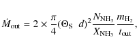
|
(1) |
where d is the distance,
Based on the previous considerations, we conclude that both infall and expansion could coexist in G10 HMC, the former involving most of the core gas, the latter being confined to narrow bipolar outflows from B1 and B2.
![\begin{figure}
\par\includegraphics[angle=0,width=8cm,clip]{12877f09.ps}
\end{figure}](/articles/aa/full_html/2010/01/aa12877-09/img72.png)
|
Figure 9: Spectra of the NH3(4,4) line towards G10.47+0.03. From top to bottom: mean (source averaged) spectrum over the HMC; beam-averaged spectra towards the absorption peaks of H II regions A, B1, and B2. The dotted profiles are the best fit obtained by taking into account the hyperfine structure. The dashed vertical line indicates the systemic velocity of the core. |
| Open with DEXTER | |
Temperature and luminosity:
using Fig. 8, one can obtain the temperature profile inside the HMC by plotting the maximum![\begin{figure}
\par\includegraphics[angle=-90,width=8cm,clip]{12877f10.ps}
\end{figure}](/articles/aa/full_html/2010/01/aa12877-09/img75.png)
|
Figure 10:
The solid curve is a plot of the NH3(4,4) line synthesised beam brightness
temperature as a function of core radius in G10; the error in this curve
equals the |
| Open with DEXTER | |
Clearly, the temperature increases outside-in.
This increase appears to be inconsistent
with the high optical depth of the NH3(4,4) line: if the core is optically
thick, only the surface should be visible and the observed
![]() should be
more or less the same at all radii. The reason why we observe a temperature
variation is probably because of clumpiness and large velocity gradients in the gas,
which allow us to glimpse beneath the HMC surface. However, this effect is diminished
to some extent at the highest column densities,
which explains why
should be
more or less the same at all radii. The reason why we observe a temperature
variation is probably because of clumpiness and large velocity gradients in the gas,
which allow us to glimpse beneath the HMC surface. However, this effect is diminished
to some extent at the highest column densities,
which explains why
![]() tends to flatten at small radii. This flattening
is also caused by beam dilution and to some emission being ``eaten''
by the absorption towards B1.
tends to flatten at small radii. This flattening
is also caused by beam dilution and to some emission being ``eaten''
by the absorption towards B1.
With this in mind, we may consider the
![]() profile in Fig. 10 as
a lower limit to the effective kinetic temperature inside the HMC.
As shown in Paper II, we now calculate the luminosity of the HMC
and compare this with other estimates. We use the approximation of a
spherical black body, whose luminosity equals
profile in Fig. 10 as
a lower limit to the effective kinetic temperature inside the HMC.
As shown in Paper II, we now calculate the luminosity of the HMC
and compare this with other estimates. We use the approximation of a
spherical black body, whose luminosity equals
![]() .
As we have seen,
.
As we have seen,
![]() is a reasonable approximation for T.
The problem is to establish which radius can be used as the ``photosphere''
of the black body. As noted in Paper I, this depends on the dust opacity in the
mid-IR, where the bulk of the black-body luminosity is emitted (the SED of a
is a reasonable approximation for T.
The problem is to establish which radius can be used as the ``photosphere''
of the black body. As noted in Paper I, this depends on the dust opacity in the
mid-IR, where the bulk of the black-body luminosity is emitted (the SED of a
![]() 100 K black body peaks at 30
100 K black body peaks at 30 ![]() m). Since a priori this radius
is unknown, we calculate
m). Since a priori this radius
is unknown, we calculate
![]() at all radii at which
at all radii at which
![]() has
been measured (dashed line in Fig. 10). To constrain the
value of R, we use the lower and upper limits to the luminosity of G10
given, respectively, by the sum of the luminosities of the embedded stars (of
spectral types O7 and O7.5,
corresponding to
has
been measured (dashed line in Fig. 10). To constrain the
value of R, we use the lower and upper limits to the luminosity of G10
given, respectively, by the sum of the luminosities of the embedded stars (of
spectral types O7 and O7.5,
corresponding to ![]()
![]()
![]() )
and the luminosity of the
associated IRAS point source (
)
and the luminosity of the
associated IRAS point source (
![]()
![]() ). The corresponding range
spanned by R is 0
). The corresponding range
spanned by R is 0
![]() 9-1.3
9-1.3
![]() .
.
We conclude that the luminosity of the HMC is very likely to be a few times
105 ![]() corresponding to an effective radius of 0.05-0.07 pc.
corresponding to an effective radius of 0.05-0.07 pc.
4.2 G31.41+0.31
4.2.1 Nature of the continuum sources
We now investigate the nature of the previously undetected continuum
sources A and B in the G31 HMC. Figure 11 shows their spectra,
which one can attempt to fit with the model already used in Sect. 4.1.1.
However, unlike the case of G10, the angular diameters obtained from the fit to the
SEDs are ![]() 0
0
![]() 5, an order of magnitude larger than those measured in
the continuum map (
5, an order of magnitude larger than those measured in
the continuum map (![]() 0
0
![]() 07; see Table 3). This strongly
suggests that the hypothesis that A and B are H II regions is wrong and
we decided not to use this model fit.
An alternative possibility is that the observed
emission originates in thermal jets. It is well known that such jets have
SEDs resembling power laws with slopes up to 1.5 (see e.g. Anglada 1996),
i.e., similar to those in Fig. 11. Moreover, jet
models predict that the angular size should decrease with increasing
frequency as a power law with an index that is found to vary with the jet
opening angle. Anglada's values range from -1.9 to -0.3.
Using the 1.3 cm and 7 mm data in
Table 3 (the resolution at 3.6 cm is insufficient to
estimate the source size), we obtain indices of -0.46 and -0.87,
respectively, for A and B, which further support the jet model.
07; see Table 3). This strongly
suggests that the hypothesis that A and B are H II regions is wrong and
we decided not to use this model fit.
An alternative possibility is that the observed
emission originates in thermal jets. It is well known that such jets have
SEDs resembling power laws with slopes up to 1.5 (see e.g. Anglada 1996),
i.e., similar to those in Fig. 11. Moreover, jet
models predict that the angular size should decrease with increasing
frequency as a power law with an index that is found to vary with the jet
opening angle. Anglada's values range from -1.9 to -0.3.
Using the 1.3 cm and 7 mm data in
Table 3 (the resolution at 3.6 cm is insufficient to
estimate the source size), we obtain indices of -0.46 and -0.87,
respectively, for A and B, which further support the jet model.
![\begin{figure}
\par\includegraphics[angle=-90,width=8cm,clip]{12877f11.ps}
\end{figure}](/articles/aa/full_html/2010/01/aa12877-09/img83.png)
|
Figure 11:
Spectral energy distributions of the continuum sources detected in the G31 HMC.
The errorbars represent a 15% calibration uncertainty.
The straight lines are least square fits to the data of the type
|
| Open with DEXTER | |
If the jet interpretation is correct, what are the masses of the powering
stars? To answer this question one can use the parameter ![]() ,
which is an estimate of the emission strength of the jet used to relate
the observed jet properties to the relevant physical parameters
of the powering source.
For G31 A and B, we have
,
which is an estimate of the emission strength of the jet used to relate
the observed jet properties to the relevant physical parameters
of the powering source.
For G31 A and B, we have
![]() mJy kpc2, which is much higher than
the values found by Anglada (1996) in their sources, namely
mJy kpc2, which is much higher than
the values found by Anglada (1996) in their sources, namely
![]() mJy kpc2. Since the latter sample comprises mostly
low- and intermediate-mass YSOs, we conclude that our objects are
high-mass YSOs.
mJy kpc2. Since the latter sample comprises mostly
low- and intermediate-mass YSOs, we conclude that our objects are
high-mass YSOs.
Extrapolating the trend in Fig. 4 of Anglada (1996), we can
derive a rough estimate of the momentum rate of the jets: this is
![]() 0.03-0.06
0.03-0.06 ![]() km s-1 yr-1, typical of high-mass YSOs (see Wu et al. 2004 and López-Sepulcre et al. 2009). Values that high
are consistent with the HMC luminosity obtained in Sect. 4.2.2
(
km s-1 yr-1, typical of high-mass YSOs (see Wu et al. 2004 and López-Sepulcre et al. 2009). Values that high
are consistent with the HMC luminosity obtained in Sect. 4.2.2
(![]()
![]() ).
).
4.2.2 Structure of the HMC
Velocity field:
as already noted in Sect. 3.2, the shape of the ammonia core in Fig. 6 is significantly elongated in the NE-SW direction. The existence of a velocity gradient in this direction was established by several authors (Cesaroni et al. 1994b; Paper II; Maxia et al. 2001; Beltrán et al. 2004, 2005; Gibb et al. 2004; Araya et al. 2008), who observed the G31 HMC at lower angular resolution than ourselves. To verify their results, in Fig. 12 we show a map of the first moment of the NH3(4,4) main line. Clearly, the velocity is increasing from NE to SW, approximately from 92 to 102 km s-1 over 1Comparing results obtained for different tracers and with different angular and spectral resolutions may lead to erroneous conclusions, and indeed the spread among the previous estimates is quite large. However, one should note that the velocity gradient obtained from our A-array measurements is by far the largest: this suggests that additional improvement in angular resolution might detect an even greater velocity spread over a smaller region. A velocity increasing with decreasing radius is indicative of conservation of angular momentum (or centrifugal equilibrium) in a rotating core. This interpretation was proposed by Beltrán et al. (2004, 2005), who modeled the CH3CN(12-11) line emission with a rotating, infalling toroid. An alternative scenario was presented by Araya et al. (2008), who interpreted their CH3OH observations as a bipolar outflow powered by a source lying between G31 A and B. We note that the argument of velocity increasing with decreasing radius is insufficient to discard the outflow interpretation, as the highest expansion speed is likely to occur close to the powering source.
Is it possible to discriminate between these two hypotheses (rotation versus expansion) on the basis of our new ammonia data?
To provide a more quantitative description of the velocity field in the
G31 HMC, in Fig. 13 we show the position-velocity plot of the
NH3(4,4) line emission along a direction with
![]() .
To
increase the signal-to-noise ratio, we averaged the emission of the HMC
along the perpendicular direction, i.e., along
.
To
increase the signal-to-noise ratio, we averaged the emission of the HMC
along the perpendicular direction, i.e., along
![]() .
The velocity
change with offset is also seen in this plot, most clearly in the main line
emission, because the satellite emission is affected by blending between the
two strongest hyperfine components inside each pair of satellites. Focusing
our attention on the main line, the shape of the plot is clearly
asymmetric along the velocity axis, with the blue-shifted emission being more
prominent than the red-shifted one.
.
The velocity
change with offset is also seen in this plot, most clearly in the main line
emission, because the satellite emission is affected by blending between the
two strongest hyperfine components inside each pair of satellites. Focusing
our attention on the main line, the shape of the plot is clearly
asymmetric along the velocity axis, with the blue-shifted emission being more
prominent than the red-shifted one.
This is also consistent with the blue-shifted velocities observed towards the centre of Fig. 12, because the first moment of the line is affected by the lack of red-shifted emission. This can be understood by looking at the NH3(4,4) spectrum obtained by averaging the emission over the HMC (Fig. 14). Here the main line peak is skewed to the blue side, as expected in collapsing optically thick envelopes. Red-shifted self-absorption can explain this asymmetry (see e.g., Myers et al. 1996 and references therein) thus suggesting that the HMC is undergoing infall (and rotation), as hypothesised by Beltrán et al. (2005).
![\begin{figure}
\par\includegraphics[angle=-90,width=8.5cm,clip]{12877f12.ps}
\end{figure}](/articles/aa/full_html/2010/01/aa12877-09/img89.png)
|
Figure 12: Map of the first moment of the NH3(4,4) main line in G31. The contour levels range from 92 (blue) to 101.8 (red) in steps of 1.4 km s-1. The two black dots mark the positions of the continuum sources A and B. The ellipse at the bottom left denotes the synthesised HPBW. |
| Open with DEXTER | |
![\begin{figure}
\par\includegraphics[angle=0,width=8.5cm,clip]{12877f13.ps}
\end{figure}](/articles/aa/full_html/2010/01/aa12877-09/img90.png)
|
Figure 13:
Plot of the NH3(4,4) line intensity as a function of LSR velocity and distance
measured along the direction with
|
| Open with DEXTER | |
![\begin{figure}
\par\includegraphics[angle=0,width=8.5cm,clip]{12877f14.ps}
\end{figure}](/articles/aa/full_html/2010/01/aa12877-09/img91.png)
|
Figure 14:
Mean spectrum of the G31 HMC, obtained by averaging the NH3(4,4) line
emission inside the |
| Open with DEXTER | |
This effect is most evident when studying the shapes of NH3(4,4)
spectra across the core. To enhance self-absorption to the
detriment of the NE-SW velocity gradient, we computed mean spectra at
radius multiples of 0
![]() 1 by averaging the emission over circular annuli
centered on the position of B1. These are shown in Fig. 15.
One can see that towards the HMC centre the ammonia main line becomes
heavily self-absorbed, becoming even weaker than the (optically thinner)
satellites. Moving outward, the main line to satellite ratio increases,
and the red-shifted self absorption in the main line disappears.
1 by averaging the emission over circular annuli
centered on the position of B1. These are shown in Fig. 15.
One can see that towards the HMC centre the ammonia main line becomes
heavily self-absorbed, becoming even weaker than the (optically thinner)
satellites. Moving outward, the main line to satellite ratio increases,
and the red-shifted self absorption in the main line disappears.
![\begin{figure}
\par\includegraphics[angle=0,width=8.5cm,clip]{12877f15.ps}
\end{figure}](/articles/aa/full_html/2010/01/aa12877-09/img92.png)
|
Figure 15: Mean spectra of the NH3(4,4) line in G31. Each spectrum refers to the angular distance from the core centre indicated in the top right of the corresponding panel. The dashed vertical line marks the systemic velocity. Note how the main line is heavily self-absorbed towards the HMC centre. |
| Open with DEXTER | |
As demonstrated in the Appendix,
a ring of molecular gas undergoing infall and rotation is described by the
expression
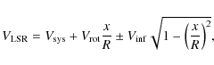
|
(2) |
where
One can estimate the mass infall rate using the mean density estimate from
Paper I (
![]() cm-3) and the values of the
infall velocity and corresponding radius obtained from the fit to the
position-velocity plot. We have
cm-3) and the values of the
infall velocity and corresponding radius obtained from the fit to the
position-velocity plot. We have
![]() yr-1. This value lies in the range
yr-1. This value lies in the range
![]() yr-1 derived by Girart et al.
(2009) from the inverse P-Cygni profile of the C34S(7-6) line, but is
an order of magnitude greater than the value of
yr-1 derived by Girart et al.
(2009) from the inverse P-Cygni profile of the C34S(7-6) line, but is
an order of magnitude greater than the value of
![]() yr-1 obtained by Osorio et al. (2009).
The latter is likely to be more reliable, as it was obtained by a model fitting
to the NH3(4,4) line profiles and the SED of the G31 region, whereas in our
calculation of
yr-1 obtained by Osorio et al. (2009).
The latter is likely to be more reliable, as it was obtained by a model fitting
to the NH3(4,4) line profiles and the SED of the G31 region, whereas in our
calculation of ![]() we used only approximate values of the radius
and density at which the infall velocity is measured. In any case, we note
that accretion rates
we used only approximate values of the radius
and density at which the infall velocity is measured. In any case, we note
that accretion rates ![]()
![]() yr-1 are not
unusual in high-mass star-forming regions (see e.g., Fontani et al.
2002; Zhang et al. 2005; Beltrán et al. 2006).
yr-1 are not
unusual in high-mass star-forming regions (see e.g., Fontani et al.
2002; Zhang et al. 2005; Beltrán et al. 2006).
In this picture, part of the infalling material accretes onto the two continuum sources, A and B, which are aligned along the plane of rotation because they form a loose binary system formed at the centre of the HMC, rotating about the same axis as the core. This finding would be consistent with the prediction of Krumholz et al. (2009). According to their numerical simulations, high-mass stars form by means of disk accretion and fragmentation of the disk yields a massive stellar companion to the primary star.
Albeit appealing, this explanation cannot exclude the outflow hypothesis. Expansion does not exclude infall, if the outflowing NH3 gas is ejected by a star that is at the same time accreting material from a compact NH3 core. In this scenario, the self-absorbed NH3 profile is caused by the infalling core, whereas the velocity gradient is caused by the expanding gas in the outflow. Other lines of evidence support the existence of an outflow in the region (see Araya et al. 2008 for a detailed discussion), such as the similar velocity gradients being measured in the SiO(2-1) and HCO+(1-0) lines (Maxia et al. 2001), which are well known jet/outflow tracers.
In this context, the two continuum sources A and B could be seen as the (unresolved) bow shocks at the two opposite ends of a thermal jet emanating from a star lying between them. The remarkable alignment between the A-B axis and the direction of the velocity gradient supports this hypothesis.
Assuming that we indeed observe a bipolar outflow lying close to the
plane of the sky, it is possible to estimate the main outflow parameters
from the gas mass associated with the NH3 high-velocity emission,
the separation between the blue- and red-shifted gas, and the corresponding
velocities. As one can see in Fig. 14, only ![]() 20% of the
NH3(4,4) emission is contained in the line wings. Assuming that the
temperature of the gas traced by the NH3(4,4) line is approximately
the same at all velocities, this implies that only
20% of the
NH3(4,4) emission is contained in the line wings. Assuming that the
temperature of the gas traced by the NH3(4,4) line is approximately
the same at all velocities, this implies that only ![]() 20% of the
core mass is undergoing expansion. The most reliable HMC mass estimate
is probably one obtained from the millimeter dust continuum (see
Beltrán et al. 2004) i.e.
20% of the
core mass is undergoing expansion. The most reliable HMC mass estimate
is probably one obtained from the millimeter dust continuum (see
Beltrán et al. 2004) i.e. ![]()
![]() .
From Fig. 13,
one can estimate an outflow size and an expansion speed, respectively,
of
.
From Fig. 13,
one can estimate an outflow size and an expansion speed, respectively,
of ![]() 0
0
![]() 8 (or 0.03 pc) and
8 (or 0.03 pc) and ![]() 4 km s-1, corresponding to a
timescale of
4 km s-1, corresponding to a
timescale of ![]() 7300 yr. This is likely to be an upper limit because of the
outflow inclination with respect to the line of sight. The mass and momentum
rates are hence >
7300 yr. This is likely to be an upper limit because of the
outflow inclination with respect to the line of sight. The mass and momentum
rates are hence >
![]() yr-1 and
>
yr-1 and
>
![]() km s-1 yr-1. Albeit large, values such as these
can be attained in the most luminous star-forming regions (see e.g.,
López-Sepulcre et al. 2009).
km s-1 yr-1. Albeit large, values such as these
can be attained in the most luminous star-forming regions (see e.g.,
López-Sepulcre et al. 2009).
In conclusion, on the basis of our new data we cannot decide whether the velocity gradient observed in G31 is due to rotation or expansion, and the debate is bound to remain open until complementary information becomes available. The polarization study by Girart et al. (2009) indicates that the magnetic field lines describe a hour-glass-shaped structure aligned SE-NW, which is consistent with the rotating toroid interpretation. Future proper motion measurements of the maser spots associated with the HMC will help us to reconstruct the 3-D velocity field of the gas, thus helping to resolve this controversy.
Temperature and luminosity:
we now proceed as for G10 to estimate the temperature profile and the luminosity of G31. Figure 16 shows the brightness temperature and the corresponding![\begin{figure}
\par\includegraphics[angle=-90,width=8.8cm,clip]{12877f16.ps}
\vspace*{4mm}
\end{figure}](/articles/aa/full_html/2010/01/aa12877-09/img106.png)
|
Figure 16:
Same as Fig. 10 for G31. The error in
|
| Open with DEXTER | |
It is not worth repeating the considerations made in Sect. 4.1.2,
which apply to G31 as well as to G10. Here, we note only that the temperature
in the outer regions is similar for the two HMCs, but the increase towards
the centre is apparently steeper in G31 than in G10, probably due to the lack
of
absorption in G31 against bright embedded continuum sources.
The luminosity of the IRAS point source associated with G31 is
![]() ,
which also includes the O6 star ionising the UC
H II to the NE of the HMC, namely
,
which also includes the O6 star ionising the UC
H II to the NE of the HMC, namely
![]() (see Table 5 and
Fig. 3d of Paper II). Hence, the HMC luminosity must be
(see Table 5 and
Fig. 3d of Paper II). Hence, the HMC luminosity must be ![]()
![]() .
This value is similar to the estimate obtained by Osorio et al.
(2009) by model fitting the SED of the HMC
and the NH3(4,4) line profiles observed in Papers I and II.
Using the same argument as for G10, we conclude that the radius of the
photosphere emitting the bulk of the HMC luminosity is of order 1
.
This value is similar to the estimate obtained by Osorio et al.
(2009) by model fitting the SED of the HMC
and the NH3(4,4) line profiles observed in Papers I and II.
Using the same argument as for G10, we conclude that the radius of the
photosphere emitting the bulk of the HMC luminosity is of order 1
![]() or
0.038 pc.
or
0.038 pc.
5 Summary and conclusions
VLA A-array observations of the NH3(4,4) line and continuum emission at various wavelengths have made it possible to shed light on the nature of the HMCs G10 and G31. Our main results are that G10 contains two deeply embedded HC H II regions (B1 and B2) associated with O9 ZAMS stars and an UC H II region (A) ionised by a B0 star located close to the HMC surface. Two weak continuum sources (A and B) have been detected inside the G31 HMC. The SEDs and the dependences of size on frequency are consistent with these sources being thermal radio jets powered by high-mass stars, rather than H II regions.
We obtain evidence of infall in both HMCs, but only in G10 do we detect expansion, possibly in two narrow bipolar outflows oriented along the line of sight. Nonetheless, we cannot exclude that the radio jets in G31 are associated with larger scale bipolar outflows, undetected in our ammonia observations.
The morphology and kinematics differ significantly from one HMC to the other. G10 appears to be spherical and to have no velocity gradient in the plane of the sky. In contrast, G31 is elongated NE-SW and the gas velocity increases systematically from SW to NE, while the NH3(4,4) main line presents red-shifted self absorption. While two competing models have been proposed to interpret this feature (rotation versus outflow), we conclude that on the basis of our data neither hypothesis can be ruled out.
The temperature structure of the two cores indicates that the total
luminosity of the embedded stars is of the order of
![]() ,
emitted mostly at a radius of 0.04-0.07 pc.
,
emitted mostly at a radius of 0.04-0.07 pc.
Table 5: Summary of the characteristics of the HMCs in G10.47+0.03 and G31.41+0.31. A ``-'' indicates that we do not have evidence in favour or against the corresponding issue.
In Table 5, we summarize and compare the main properties of the two HMCs. Despite the similarities, one can see a few noticeable differences. Here, we attempt to elaborate a simple scenario accounting for them. In particular, one striking difference is that no detectable H II region is present in G31, although the luminosity (and the HMC mass; see Paper I) of the latter is only a few times less than that of the former. Why is this so? We can imagine two possible explanations:
- (i)
- G10 is older than G31. In this case, the embedded early-type stars in the latter object are in a pre-H II region phase, which is why we detect only faint radio emission from them.
- (ii)
- The most massive stars in G31 are less massive than those in G10. This may occur if, for purely statistical reasons, the initial mass function (IMF) in G31 is biased towards low stellar masses.
The former hypothesis, instead, is consistent with our findings. In
particular, the lack of a HC H II region can be justified by the presence of
accretion at a rate sufficiently high to trap the ionised gas
(Keto 2002) or even inhibit its formation (Yorke 1985).
We note that the rate of ![]() 0.019
0.019 ![]() yr-1 estimated in
Sect. 4.2.2 is enough to quench an H II region around any early-type
star, provided that the accretion has spherical symmetry.
yr-1 estimated in
Sect. 4.2.2 is enough to quench an H II region around any early-type
star, provided that the accretion has spherical symmetry.
If our interpretation is correct, one can speculate that G31 is in an earlier evolutionary phase than G10, when heavy accretion from a rotating/collapsing envelope onto a newly formed high-mass (proto)star is going on. At this stage, a thermal jet develops before the star is capable of ionising its molecular surroundings.
G10 could instead represent a later evolutionary phase, when the accreting material is partly diverted into a dense collimated jet digging its way through the parental core. Following Keto (2007), the presence of lower density channels and the increased stellar mass could allow the development of an untrapped HC H II region, which is bound to expand and eventually destroy the HMC.
Although highly speculative, the scenario depicted above is consistent with all of our findings. We believe that answering the questions concerning the nature and age of HMCs will not take too long. With the advent of ALMA, the number of observable tracers will increase enormously, as well as the angular and spectral resolution attainable. These dramatic improvements will provide us with suitable tools to solve the problem of high-mass star formation.
AcknowledgementsIt is a pleasure to thank Maite Beltrán for critically reading the manuscript. P.H. acknowledges partial support from NSF grant AST-0908901.
Appendix A: Line-of-sight velocity of rotating ring
The purpose of this Appendix is to derive the expression of the velocity
along the line of sight of a rotating and infalling ring seen edge-on.
In Fig. A.1, a sketch of the ring of radius Rand associated rotation (
![]() )
and
infall (
)
and
infall (
![]() )
velocities is shown. The velocity measured by an observer
located at
)
velocities is shown. The velocity measured by an observer
located at ![]() is the sum of the components along z of
is the sum of the components along z of
![]() and
and
![]() ,
plus the systemic velocity of the whole ring
with respect to the local standard of rest (
,
plus the systemic velocity of the whole ring
with respect to the local standard of rest (
![]() ):
):
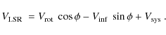
|
(A.1) |
Using the expressions
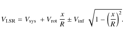
![\begin{figure}
\par\includegraphics[angle=0,width=8.8cm]{12877f17.ps}
\end{figure}](/articles/aa/full_html/2010/01/aa12877-09/img114.png)
|
Figure A.1:
Sketch of a rotating and infalling ring of radius R seen edge on by an
observer located at |
| Open with DEXTER | |
References
- Anglada, G. 1996, ASP Conf. Ser., 93, 3 [NASA ADS] [Google Scholar]
- Araya, E., Hofner, P., Kurtz, S., Olmi, L., & Linz, H. 2008, ApJ, 675, 420 [NASA ADS] [CrossRef] [Google Scholar]
- Beltrán, M. T., Cesaroni, R., Neri, R., et al. 2004, ApJ, 601, L187 [NASA ADS] [CrossRef] [Google Scholar]
- Beltrán, M. T., Cesaroni, R., Neri, R., et al. 2005, A&A, 435, 901 [Google Scholar]
- Beltrán, M. T., Cesaroni, R., Codella, C., et al. 2006, Nature, 443, 427 [NASA ADS] [CrossRef] [PubMed] [Google Scholar]
- Beuther, H., Churchwell, E. B., McKee, C. F., & Tan, J. C. 2007, in Protostars and Planets V, ed. B. Reipurth, D. Jewitt, & K. Keil (Tucson: Univ. of Arizona Press), 165 [Google Scholar]
- Cesaroni, R. 2005, in Massive Star Birth: a Crossroads of Astrophysics, ed. R. Cesaroni, M. Felli, E. Churchwell, & M. Walmsley (Cambridge University Press), IAU Symp., 227, 59 [Google Scholar]
- Cesaroni, R., Churchwell, E., Hofner, P., Walmsley, C. M., & Kurtz, S. 1994a, A&A, 288, 903 (Paper I) [Google Scholar]
- Cesaroni, R., Olmi, L., Walmsley, C. M., Churchwell, E., & Hofner, P. 1994b, ApJ, 435, L137 [NASA ADS] [CrossRef] [Google Scholar]
- Cesaroni, R., Hofner, P., Walmsley, C. M., & Churchwell, E. 1998, A&A, 331, 709 (Paper II) [Google Scholar]
- Cesaroni, R., Galli, D., Lodato, G., Walmsley, C. M., & Zhang, Q. 2007, in Protostars and Planets V, ed. B. Reipurth, D. Jewitt, & K. Keil (Tucson: Univ. of Arizona Press), 197 [Google Scholar]
- Churchwell, E., Walmsley, C. M., & Cesaroni, R. 1990, A&AS, 83, 119 [Google Scholar]
- Franco, J., Tenorio-Tagle, G., & Bodenheimer, P. 1990, ApJ, 349, 126 [NASA ADS] [CrossRef] [Google Scholar]
- Furuya, R. S., Cesaroni, R., Takahashi, S., et al. 2005, ApJ, 624, 827 [NASA ADS] [CrossRef] [Google Scholar]
- Fontani, F., Cesaroni, R., Caselli, P., & Olmi, L. 2002, A&A, 389, 603 [Google Scholar]
- Gibb, A. G., Wyrowski, F., & Mundy, L. G. 2004, ApJ, 616, 301 [NASA ADS] [CrossRef] [Google Scholar]
- Girart, J. M., Beltrán, M. T., Zhang, Q., Rao, R., & Estalella, R. 2009, Science, 324, 1408 [NASA ADS] [CrossRef] [PubMed] [Google Scholar]
- Hoare, M. G., Kurtz, S., Lizano, S., Keto, E., & Hofner, P. 2007, in Protostars and Planets V, ed. B. Reipurth, D. Jewitt, & K. Keil (Tucson: Univ. of Arizona Press), 181 [Google Scholar]
- Keto, E. H. 2002, ApJ, 580, 980 [NASA ADS] [CrossRef] [Google Scholar]
- Keto, E. H. 2003, ApJ, 599, 1196 [NASA ADS] [CrossRef] [Google Scholar]
- Keto, E. H. 2007, ApJ, 666, 976 [NASA ADS] [CrossRef] [Google Scholar]
- Keto, E. H., & Wood, K. 2006, ApJ, 637, 850 [NASA ADS] [CrossRef] [Google Scholar]
- Krumholz, M. R., Klein, R. I., McKee, C. F., Offner, S. S. R., & Cunningham, A. J. 2009, Science, 323, 754 [NASA ADS] [CrossRef] [PubMed] [Google Scholar]
- Kurtz, S., Cesaroni, R., Churchwell, E., Hofner, P., & Walmsley, C. M. 2000, in Protostars and Planets IV, ed. V. Mannings, A. Boss, & S. Russel (Tucson: Univ. of Arizona Press), 299 [Google Scholar]
- López-Sepulcre, A., Codella, C., Cesaroni, R., Marcelino, N., & Walmsley, C. M. 2009, A&A, 499, 811 [Google Scholar]
- Martins, F., Schaerer, D., & Hillier, D. J. 2002, A&A, 382, 999 [Google Scholar]
- Maxia, C., Testi, L., Cesaroni, R., & Walmsley, C. M. 2001, A&A, 371, 287 [Google Scholar]
- Myers, P. C., Mardones, D., Tafalla, M., Williams, J. P., & Wilner, D. J. 1996, ApJ, 465, L133 [NASA ADS] [CrossRef] [Google Scholar]
- Olmi, L., Cesaroni, R., & Walmsley, C. M. 1996a, A&A, 307, 599 [Google Scholar]
- Olmi, L., Cesaroni, R., Neri, R., & Walmsley, C. M. 1996b, A&A, 315, 565 [Google Scholar]
- Osorio, M., Anglada, G., Lizano, S., & D'Alessio, P. 2009, ApJ, 694, 29 [NASA ADS] [CrossRef] [Google Scholar]
- Panagia, N. 1973, AJ, 78, 929 [NASA ADS] [CrossRef] [Google Scholar]
- Panagia, N., & Felli, M. 1975, A&A, 39, 1 [Google Scholar]
- Pandian, J. D., Momjian, E., & Goldsmith, P. F. 2008, A&A, 486, 191 [Google Scholar]
- Poynter, R. L., & Kakar, R. K. 1975, ApJS, 29, 87 [NASA ADS] [CrossRef] [Google Scholar]
- Sewilo, M., Watson, C., Araya, E., et al. 2004, ApJ, 154, 553 [Google Scholar]
- Ungerechts, H., Walmsley, C. M., & Winnewisser, G. 1986, A&A, 157, 207 [Google Scholar]
- Van Dishoeck, E. F., Blake, G. A., Draine, B. T., & Lunine, J. I. 1993, Protostars and Planets III, ed. E. H. Levy, & J. I. Lunine (Tucson: Univ. of Arizona Press), 163 [Google Scholar]
- Wilner, D. J., De Pree, C. G., Welch, W. J., & Goss, W. M. 2001, ApJ, 550, L81 [NASA ADS] [CrossRef] [Google Scholar]
- Wood, D. O. S., & Churchwell, E. 1989, ApJ, 69, 831 [NASA ADS] [Google Scholar]
- Wu, Y., Wei, Y., & Zhao, M. 2004, A&A, 426, 503 [Google Scholar]
- Yorke, H. W. 1985, in Birth and Infancy of Stars, 645 [Google Scholar]
- Zhang, Q. 2005, in Massive Star Birth: a Crossroads of Astrophysics, ed. R. Cesaroni, M. Felli, E. Churchwell, & M. Walmsley (Cambridge University Press), IAU Symp., 227, 135 [Google Scholar]
Footnotes
- ... 1000 AU
- Based on observations carried out with the NRAO Very Large Array. The National Radio Astronomy Observatory is operated by Associated Universities, Inc., under cooperative agreement with the National Science Foundation.
- ... quantities
- Note that in Papers I and II a distance of 5.8 kpc was adopted for G10.
- ...1973)
- We prefer to use Panagia's estimates rather than more recent ones for the sake of consistency with Paper II. Note that the variation in the estimated spectral type would not be significant: e.g., using the results of Martins et al. (2002) would affect only the spectral type of G10 B2, which would change from O7.5 to O8.
All Tables
Table 1: Parameters of VLA observations.
Table 2: Observed parameters of the continuum sources in G10.47+0.03.
Table 3: Observed parameters of the continuum sources in G31.41+0.31.
Table 4: Parameters of the H II regions and corresponding ionising stars in G10.47+0.03. A distance of 10.8 kpc is adopted.
Table 5: Summary of the characteristics of the HMCs in G10.47+0.03 and G31.41+0.31. A ``-'' indicates that we do not have evidence in favour or against the corresponding issue.
All Figures
|
|
Figure 1: Images of the continuum emission towards G10.47+0.03. In the bottom left of each panel, the observing wavelength is indicated. Letters A, B1, B2, and D denote the different sources detected in the region. Contour levels range from 1.1 to 14.96 in steps of 1.98 mJy/beam at 6 cm, from 0.3 to 1.5 in steps of 0.6 mJy/beam and from 3.3 to 15.9 in steps of 1.8 mJy/beam at 3.6 cm, from 3.45 to 46.92 in steps of 6.21 mJy/beam at 2 cm, and from 1.25 to 10.25 in steps of 2.25 mJy/beam at 1.3 cm. |
| Open with DEXTER | |
| In the text | |
|
|
Figure 2: Top: overlay of the 1.3 cm continuum map (contours) on the image of the 7 mm continuum emission (colour scale). The contour levels range from 0.126 to 0.432 in steps of 0.102 mJy/beam. The ellipses to the bottom left and right represent the synthesised beams at 1.3 cm and 7 mm, respectively. Bottom: same as top, where the 1.3 cm emission is replaced by that at 3.6 cm. The contour levels range from 0.033 to 0.297 in steps of 0.066 mJy/beam. The ellipse represents the synthesised beam at 3.6 cm. |
| Open with DEXTER | |
| In the text | |
|
|
Figure 3: Top: overlay of the 1.3 cm continuum map (contours, as in Fig. 1) on the image of the NH3(4,4) emission averaged under the main line in G10. Bottom: same as above for the NH3(4,4) emission averaged under the four satellites. Note that both colour scales have been clipped at -0.4 mJy/beam to enhance the contrast of the images. The ellipse at the bottom right denotes the synthesised beam of the ammonia maps. |
| Open with DEXTER | |
| In the text | |
|
|
Figure 4: Top: overlay of the 1.3 cm continuum map (contours, as in Fig. 2) in the image of the NH3(4,4) emission averaged over the main line in G31. Bottom: same as above for the NH3(4,4) emission averaged under the four satellites. The ellipse at the bottom right denotes the synthesised beam of the ammonia maps. |
| Open with DEXTER | |
| In the text | |
|
|
Figure 5: Top: map of the NH3(4,4) emission averaged under the main line in G10. Middle: map of the NH3(4,4) emission averaged under the four satellites. Bottom: map of the ratio between the main line and satellite maps. A ratio <37 implies that the main line is optically thick, <1.6 that also the satellite emission is thick. Note that the maximum ratio is 5.8, but the colour scale has been clipped at 3 to enhance the contrast of the image. The two circles mark the positions of the HC H II regions B1 and B2. The values of the contours are marked in the colour-scale wedges to the right of each panel. The ellipse at the bottom right denotes the synthesised beam of the ammonia maps. |
| Open with DEXTER | |
| In the text | |
|
|
Figure 6: Top: map of the NH3(4,4) emission averaged under the main line in G31. Middle: map of the NH3(4,4) emission averaged under the four satellites. Bottom: map of the ratio between the main line and satellite maps. A ratio <37 implies that the main line is optically thick, <1.6 that also the satellite emission is thick. The values of the contours are marked in the colour-scale wedges to the right of each panel. The ellipse at the bottom right denotes the synthesised beam of the ammonia maps. |
| Open with DEXTER | |
| In the text | |
|
|
Figure 7: Spectral energy distributions of the continuum sources detected in the G10 HMC. Note that the 1.3 cm flux is not the one given in Table 2 (where most of the emission is resolved out) but that obtained from our old B-array data. The errorbars allow for 15% calibration uncertainty. The curves represent the best fit to the data using a model of an H II region with a density gradient (see text). |
| Open with DEXTER | |
| In the text | |
|
|
Figure 8: Plot of the NH3(4,4) line intensity as a function of LSR velocity and distance from the centre of the HMC in G10, assumed to coincide with the HC H II region B1. Contour levels range from -10.9 to -0.4 in steps of 1.5 mJy/beam and from 0.4 to 1.6 in steps of 0.3 mJy/beam. The dashed horizontal lines mark the positions of the main line and strongest satellites. The cross at the bottom right indicates the angular and spectral resolutions. |
| Open with DEXTER | |
| In the text | |
|
|
Figure 9: Spectra of the NH3(4,4) line towards G10.47+0.03. From top to bottom: mean (source averaged) spectrum over the HMC; beam-averaged spectra towards the absorption peaks of H II regions A, B1, and B2. The dotted profiles are the best fit obtained by taking into account the hyperfine structure. The dashed vertical line indicates the systemic velocity of the core. |
| Open with DEXTER | |
| In the text | |
|
|
Figure 10:
The solid curve is a plot of the NH3(4,4) line synthesised beam brightness
temperature as a function of core radius in G10; the error in this curve
equals the |
| Open with DEXTER | |
| In the text | |
|
|
Figure 11:
Spectral energy distributions of the continuum sources detected in the G31 HMC.
The errorbars represent a 15% calibration uncertainty.
The straight lines are least square fits to the data of the type
|
| Open with DEXTER | |
| In the text | |
|
|
Figure 12: Map of the first moment of the NH3(4,4) main line in G31. The contour levels range from 92 (blue) to 101.8 (red) in steps of 1.4 km s-1. The two black dots mark the positions of the continuum sources A and B. The ellipse at the bottom left denotes the synthesised HPBW. |
| Open with DEXTER | |
| In the text | |
|
|
Figure 13:
Plot of the NH3(4,4) line intensity as a function of LSR velocity and distance
measured along the direction with
|
| Open with DEXTER | |
| In the text | |
|
|
Figure 14:
Mean spectrum of the G31 HMC, obtained by averaging the NH3(4,4) line
emission inside the |
| Open with DEXTER | |
| In the text | |
|
|
Figure 15: Mean spectra of the NH3(4,4) line in G31. Each spectrum refers to the angular distance from the core centre indicated in the top right of the corresponding panel. The dashed vertical line marks the systemic velocity. Note how the main line is heavily self-absorbed towards the HMC centre. |
| Open with DEXTER | |
| In the text | |
|
|
Figure 16:
Same as Fig. 10 for G31. The error in
|
| Open with DEXTER | |
| In the text | |
|
|
Figure A.1:
Sketch of a rotating and infalling ring of radius R seen edge on by an
observer located at |
| Open with DEXTER | |
| In the text | |
Copyright ESO 2010
Current usage metrics show cumulative count of Article Views (full-text article views including HTML views, PDF and ePub downloads, according to the available data) and Abstracts Views on Vision4Press platform.
Data correspond to usage on the plateform after 2015. The current usage metrics is available 48-96 hours after online publication and is updated daily on week days.
Initial download of the metrics may take a while.