| Issue |
A&A
Volume 509, January 2010
|
|
|---|---|---|
| Article Number | A37 | |
| Number of page(s) | 8 | |
| Section | Celestial mechanics and astrometry | |
| DOI | https://doi.org/10.1051/0004-6361/200912691 | |
| Published online | 14 January 2010 | |
Gaia relativistic astrometric models
I. Proper stellar direction and aberration
M. Crosta - A. Vecchiato
INAF - Astronomical Observatory of Torino, via Osservatorio 20, 10025 Pino Torinese (TO), Italy
Received 12 June 2009 / Accepted 5 October 2009
Abstract
The high accuracy achievable by modern space astrometry requires
the use of General Relativity to model the stellar light propagation
through the gravitational field encountered from a source to a given
observer inside the Solar System. The general relativistic definition
of an astrometric measurement needs an appropriate use of the concept
of reference frame, which should then be linked to the conventions of
the IAU resolutions. On the other hand, a definition of the astrometric
observables in the context of General Relativity is also essential for
finding the stellar coordinates and proper
motion uniquely, this being the main physical task of the inverse
ray-tracing problem. The aim of this work is to set the level of
reciprocal consistency
of two relativistic models, GREM and RAMOD (Gaia, ESA mission), in
order to guarantee a physically correct definition of
the light's local direction to a star and deduce the star coordinates
and proper motions at the level of accuracy required by these models
consistently with the IAU's adopted reference systems.
Key words: relativity - astrometry - gravitation - reference systems - methods: data analysis - techniques: high angular resolution
1 Introduction
The correct definition of a physical measurement requires identification of an appropriate reference frame. This also applies to determining the position and motion of a star from astrometric observations made from within our Solar System. Moreover, modern instruments housed in space-borne astrometric probes like Gaia (Turon et al. 2005) and SIM (Unwin et al. 2008) aim to be accurate at the micro-arcsecond level, or higher as in the case of bright stars observed by SIM (0.2 micro-arcsecond), thus requiring that any astrometric measurement be modeled in a way that both light propagation and detection should be conceived in a general relativistic framework. One needs, in fact, to solve the relativistic equations of the null geodesic that describe the trajectory of a photon emitted by a star and detected by an observer with an assigned state of motion. The whole process takes place in a geometrical environment generated by an N-body distribution such as for our Solar System. Essential to the solution of the above astrometric problem (inverse ray tracing from observational data) is the identification, as boundary conditions, of the local observer's line-of-sight defined in a suitable reference frame (Bini et al. 2003; de Felice & Preti 2006; de Felice et al. 2006).
Summarizing from the quoted references, the astrometric problem consists of determining the astrometric parameters of a star (its coordinates, parallax, and proper motion) from a prescribed set of observational data (hereafter observables). However, while these quantities are well defined in classical (non relativistic) astrometry, in General Relativity (GR) they must be interpreted consistently with the relativistic framework of the model. Similarly, the parameters describing the attitude and the center-of-mass motion of the satellite need to be defined consistently with the chosen relativistic model.
As far as Gaia is concerned, at present two conceptual
frameworks are able to treat the astrometric problem at the
micro-arcsecond level within a relativistic context. The first model,
named GREM (Gaia RElativistic Model) and described in Klioner (2003), is an extension of a seminal study by Klioner & Kopeikin (1992)
conducted in the framework of the
post-Newtonian (pN) approximation of GR. GREM has been formulated
according to a parametrized post-Newtonian scheme accurate to
1 micro-arcsecond. In this model finite dimensions and angular
momentum
of the bodies of the Solar System are included and linked to the motion
of the observer in order to consider the effects of parallax,
aberration,
and proper motion, and the light path is solved using a matching
technique that links the perturbed internal solution inside the near
zone![]() of the Solar System with the (assumed) flat external one.
of the Solar System with the (assumed) flat external one.
Basically, the pN approach (and post-Minkowskian one, pM, as in Kopeikin & Mashhoon 2002) solves the light trajectory as a straight line (Euclidean geometry) plus integrals, containing the perturbations encountered, from a gravitating source at an arbitrary distance from an observer located within the Solar System. This allows one to transform the observed light ray in a suitable coordinate direction and to read off the aberrational terms and light deflections effects, evaluated at the point of observation. This model is considered as baseline for the Gaia data reduction.
The second model, RAMOD, is an astrometric model conceived
to solve the inverse ray-tracing problem in a general relativistic
framework not constrained by a priori approximations. RAMOD is actually
a family of models of increasing intrinsic accuracy, all based on the
geometry of curved manifolds (de Felice et al. 2004,2006).
As in Kopeikin & Mashhoon (2002),
the full development to the micro-arcsecond level imposes consideration
of the retarded distance effects by the motion of the bodies of the
Solar System. At present, the RAMOD full solution requires numerical
integration of a set of coupled nonlinear differential
equations (also called ``master equations''![]() ),
which allows the light trajectory to be traced back to the initial
position
of the star and which naturally entangles the contributions by the
aberration and those by the curvature of the background geometry. RAMOD
is formulated with a completely different methodology. This makes its
comparison with the former one a difficult
task.
),
which allows the light trajectory to be traced back to the initial
position
of the star and which naturally entangles the contributions by the
aberration and those by the curvature of the background geometry. RAMOD
is formulated with a completely different methodology. This makes its
comparison with the former one a difficult
task.
Despite its difficulty, this comparison is a necessity, beacuse GREM and RAMOD will be used for the Gaia data reduction with the purpose of creating a catalog of one billion positions and proper motions based on measurements of absolute astrometry, so any inconsistency in the relativistic model(s) would invalidate the quality and reliability of the estimates, hence all related scientific output.
In this paper we present the first step in the theoretical comparison, showing how it is possible to isolate the aberration terms from the global RAMOD construct (which are normally entangled together with other terms such as those of the deflection) and recasting them in a GREM-like formula.
In Sect. 2 we review all the building steps of the RAMOD astrometric set-up. In Sect. 3 we show the procedures used in RAMOD to define the observables and compare the quantities of GREM-like formulations by making the aberration part in the RAMOD framework explicit. Sect. 4 will comment on the results of the comparison and on what has to be addressed to proceed with the theoretical comparison of the two models. Finally, Appendix B reports the calculations of the pN/pM approaches recovering the stellar aberration.
Throughout the paper, regular bold indicates four-vector (e.g. ![]() )
and italic bold indicates three-vector (e.g.
)
and italic bold indicates three-vector (e.g. ![]() );
the components of vectorial quantities are indicated with indexes (no
bold symbols), where the Latin index stands for 1, 2, 3 and the
Greek ones for 0, 1, 2, 3. A repeated index means Einstein
summation convention and indexes are raised and lowered with the metric
);
the components of vectorial quantities are indicated with indexes (no
bold symbols), where the Latin index stands for 1, 2, 3 and the
Greek ones for 0, 1, 2, 3. A repeated index means Einstein
summation convention and indexes are raised and lowered with the metric
![]() (in particular, ni ni stands for the scalar product with respect to the Euclidean metric
(in particular, ni ni stands for the scalar product with respect to the Euclidean metric
![]() ,
whereas
,
whereas
![]() with respect to the metric
with respect to the metric
![]() ). The speed of light is symbolized by c, notations like
). The speed of light is symbolized by c, notations like ![]() indicate a set of quantities (e.g.
indicate a set of quantities (e.g.
![]() ), and
), and
![]() or
or
![]() an operator projecting with respect to the observer
an operator projecting with respect to the observer ![]() .
.
2 The RAMOD frames
In order to bring out the different methodologies and mathematical constructs applied in RAMOD, this section summarizes the set-up of RAMOD by focusing on the reference frames needed to define the measurements.
The set-up of any astrometric model primarily implies the
identification
of the gravitational sources and of the background geometry. Then
one needs to label the space-time points with a coordinate system.
These steps allow us to fix a reference frame with respect to
which one describes the light trajectory, the motion of the stars,
and that of the observer. The RAMOD framework is based on the
weak-field requirement for the background geometry, which in turn have
to be
specialized to the particular case one wants to model. For example,
keeping in mind a Gaia-like mission, we can assume the Solar System
is the only source of gravity, i.e. a physical system gravitationally
bound, in the weak field and slow motion regime. Then, only first-order
terms in the metric perturbation h (or equivalently in the constant G as in the pM approximation) are retained. These terms already include all of the possible (v/c)n-order expansions of the pN approach, but just those up to (v/c)3
are needed to reach the micro-arcsecond accuracy required for the next
generation astrometric missions, like e.g. Gaia and SIM. With these
assumptions the background geometry is given by the following
line element
where
where
2.1 The BCRS
In RAMOD, a Barycentric Celestial Reference System
(BCRS, Soffel et al. 2003) is identified requiring that a smooth family of space-like hyper-surfaces exists with the equation
![]() (see de Felice et al. 2004). The function t can be taken as a time coordinate. On each of these
(see de Felice et al. 2004). The function t can be taken as a time coordinate. On each of these
![]() hypersurfaces, one can choose a set of Cartesian-like coordinates centered
at the barycenter of the Solar System (B) and running smoothly as
parameters along space-like curves that point to distant cosmic sources.
The latter are chosen to assure that the system is kinematically
nonrotating, i.e. nonrotating with respect to the reference distant sources as recommended by the IAU (Soffel et al. 2003).
The parameters x, y, z, together with the time
coordinate t, provide a basic coordinate representation of the
space-time according to the IAU resolutions
hypersurfaces, one can choose a set of Cartesian-like coordinates centered
at the barycenter of the Solar System (B) and running smoothly as
parameters along space-like curves that point to distant cosmic sources.
The latter are chosen to assure that the system is kinematically
nonrotating, i.e. nonrotating with respect to the reference distant sources as recommended by the IAU (Soffel et al. 2003).
The parameters x, y, z, together with the time
coordinate t, provide a basic coordinate representation of the
space-time according to the IAU resolutions![]() .
.
Any tensorial quantity will be expressed in terms of coordinate components relative to coordinate bases induced by the BCRS.
2.2 The local BCRS
As shown in detail in (de Felice et al. 2004,2006), in RAMOD at any space-time point a unitary four-vector exists
![]() that is tangent to the world line of a physical observer at rest with respect to the spatial grid of the BCRS defined as
that is tangent to the world line of a physical observer at rest with respect to the spatial grid of the BCRS defined as
The totality of these four vectors over the space-time forms a vector field that is proportional to a time-like and asymptotically Killing vector field
![\begin{figure}
\par\includegraphics[width=7.5cm,clip]{12691fg1.eps}
\end{figure}](/articles/aa/full_html/2010/01/aa12691-09/img30.png)
|
Figure 1:
The local observer |
| Open with DEXTER | |
The tetrad associated to the local BCRS has spatial axes (the triad) coinciding with the local coordinate
axes, but its origin is the barycenter of the satellite. At the
![]() ,
this triad is (Bini et al. 2003)
,
this triad is (Bini et al. 2003)
Let us stress that
2.3 The proper reference frame for the satellite
The proper reference frame of a satellite consists of its rest-space
and a clock that measures the satellite proper time. The tensorial quantity that expresses a proper reference frame of
a given observer is a tetrad adapted to that observer, namely
a set of four unitary, mutually orthogonal four-vectors
![]() ,
one of which, i.e.
,
one of which, i.e.
![]() ,
is the
observer's four-velocity, while the other
,
is the
observer's four-velocity, while the other
![]() s
form a spatial triad of space-like four-vectors (Misner et al. 1973). The physical measurements made by the observer (satellite) represented
by such a tetrad are obtained by projecting the appropriate tensorial
quantities on the tetrad axes.
s
form a spatial triad of space-like four-vectors (Misner et al. 1973). The physical measurements made by the observer (satellite) represented
by such a tetrad are obtained by projecting the appropriate tensorial
quantities on the tetrad axes.
The same measurements can also be defined by splitting the space-time
into two subspaces, as sketched in Appendix A.
Essentially, this last method is useful when we do not know the
solution of a tetrad, which depends on the metric, and we only need
to know the moduli of the physical quantities. As far
as RAMOD is concerned, given the metric (1) and
in the case of a Gaia-like mission, an explicit analytic expression
for a tetrad adapted to the satellite four-velocity exists and can
be found in Bini et al. (2003). The spatial axes of this
tetrad, named
![]() ,
are used to
model the attitude of the satellite.
,
are used to
model the attitude of the satellite.
2.3.1 Satellite proper reference frame and IAU conventions
In RAMOD the satellite reference frame is obtained by successive transformations of the local BCRS tetrad
![]() as defined in Eq. (3).
In particular, the vectors of the triad
as defined in Eq. (3).
In particular, the vectors of the triad
![]() are boosted to the satellite rest-frame by means of an instantaneous Lorentz transformation (Bini et al. 2003, and reference therein),
which depends on the relative spatial velocity
are boosted to the satellite rest-frame by means of an instantaneous Lorentz transformation (Bini et al. 2003, and reference therein),
which depends on the relative spatial velocity
![]() of the satellite
of the satellite
identified by the four-velocity
The boosted tetrad
![]() obtained in this way represents a CoMRS (Center-of-Mass Reference System, comoving with the satellite), similar to what is defined for Gaia (Klioner 2004; Bastian 2004). In
addition to the definition in the cited works, one of the axes is Sun-locked,
i.e. one axis points toward the Sun at any point of its Lissajous
orbit around L2. The Gaia attitude frame is finally obtained by applying the following rotations to the
Sun-locked frame: (i) by an angle
obtained in this way represents a CoMRS (Center-of-Mass Reference System, comoving with the satellite), similar to what is defined for Gaia (Klioner 2004; Bastian 2004). In
addition to the definition in the cited works, one of the axes is Sun-locked,
i.e. one axis points toward the Sun at any point of its Lissajous
orbit around L2. The Gaia attitude frame is finally obtained by applying the following rotations to the
Sun-locked frame: (i) by an angle
![]() about the four-vector
about the four-vector
![]() which constantly points towards the Sun (where
which constantly points towards the Sun (where
![]() is the
angular velocity of precession); (ii) by a fixed angle
is the
angular velocity of precession); (ii) by a fixed angle ![]() about the image of the four-vector
about the image of the four-vector
![]() after the previous rotation; and (iii) by an angle
after the previous rotation; and (iii) by an angle
![]() about the image of the four-vector
about the image of the four-vector
![]() after the previous two rotations (where
after the previous two rotations (where
![]() is now the spin angular velocity). The triad resulting from these transformations establishes the satellite attitude triad, given by
is now the spin angular velocity). The triad resulting from these transformations establishes the satellite attitude triad, given by
The final triad
To complete the process one has to include the transformations between
the observer's proper time and the barycentric coordinate time. This can be
done using the subspace splitting technique cited in Appendix A. Let us consider the satellite's world-line in the space-time geometry as
where
Then, by inserting the last expression (6) in Eq. (A.3), we obtain the formula which ties the running between the clock on board up to the order (v/c)4and that for the origin of the BCRS:
![$\displaystyle -u_{s}^{0}\left[\left(g_{00}+\frac{v^{i}}{c}g_{i0}\right)+\frac{1}{c}g_{i0}{\rm d}x^{i}+g_{ij}\frac{v^{i}}{c}{\rm d}x^{j}\right]$](/articles/aa/full_html/2010/01/aa12691-09/img61.png)
![$\displaystyle {\rm d}t-c^{-2}\left[\left(\frac{v^{2}}{2}+w\right)+v^{i}{\rm d}R^{i}\right]$](/articles/aa/full_html/2010/01/aa12691-09/img62.png)
![$\displaystyle \left.+4w^{i}{\rm d}R^{i}-\left(3w+\frac{v^{2}}{2}\right)v^{i}{\rm d}R^{i}\right],$](/articles/aa/full_html/2010/01/aa12691-09/img64.png)
where xi is any spatial location inside or in the neighborhood of the satellite and Rsi=xi - xsi. It is trivial to check that, when we make a first-order Taylor series expansion around the satellite barycenter location
|
Equation (7) can be transformed (Crosta 2003) in the relationships between the proper time on board the satellite and the barycentric coordinate time interval as reported in IAU resolutions B1.5. This finally completes the definition of the proper reference frame for the Gaia-like satellite in the RAMOD framework and, moreover, gives proof of the compatibility of the RAMOD formalism with the IAU conventions (hence with a GREM-like approach).
3 Multi-step application of the observable e in RAMOD to the aberration
The classical (non relativistic) approach of astrometry has traditionally privileged a ``multi-step'' definition of the observable; i.e., the quantities that ultimately enter the ``final'' catalog and are referred to a global inertial reference system, are obtained taking into account effects such as aberration and parallax, one by one and independent from each other.
GREM reproduces this approach of classical astrometry in a relativistic framework. For this model the BCRS is the equivalent of the inertial reference system of the classical approach, while the final expression of the star direction in the BCRS is obtained after converting the observed direction into coordinate ones in several steps that divide the effects of the aberration, the gravitational deflection, the parallax, and proper motion (Klioner 2003) (see Appendix B). As is well known, stellar aberration arises from the motion of the observer relative to the BCRS origin, assumed to coincide with the center of mass of the Solar System.
In the previous section we mentioned that RAMOD relies on the
tetrad formalism for the definition of the observable. In general,
the three direction cosines that identify the local line-of-sight
to the observed object are relative to a spatial triad
![]() associated with a given observer
associated with a given observer ![]() ;
the direction cosines
with respect to the axes of this triad are defined as
;
the direction cosines
with respect to the axes of this triad are defined as
where the final
3.1 Attitude-free tetrad for the aberration
Whatever tetrad we consider, the expression of Eq. (8) for the
relativistic observable in the RAMOD model can also be written as (de Felice et al. 2006)
where
where
To retrieve the aberration effect given by the motion of the satellite
with respect to the BCRS in RAMOD, one needs to specialize Eq. (9)
to the case of a tetrad
![]() adapted to the center of mass of the satellite assumed with no attitude
parameters. In this case, in fact, the observation equation will give
a relation between the ``aberrated'' direction represented by
the direction cosines ea, as measured by the satellite
and the ``aberration-free'' direction given by the quantity
adapted to the center of mass of the satellite assumed with no attitude
parameters. In this case, in fact, the observation equation will give
a relation between the ``aberrated'' direction represented by
the direction cosines ea, as measured by the satellite
and the ``aberration-free'' direction given by the quantity
![]() referring to the local BCRS frame
referring to the local BCRS frame
![]() .
The
vectors of the triad
.
The
vectors of the triad
![]() differ from the local BCRS's
differ from the local BCRS's
![]() for a boost transformation with four-velocity
for a boost transformation with four-velocity
![]() .
This
means that it can be derived from Eq. (3)
using the relation (Jantzen et al. 1992)
.
This
means that it can be derived from Eq. (3)
using the relation (Jantzen et al. 1992)
![$\displaystyle \tilde{\lambda}_{\hat{a}}^{\alpha}=P\left(\vec{u_{s}}\right)_{\si...
...amma}{\gamma+1}\nu^{\sigma}\left(\nu^{\rho}\lambda_{\rho\hat{a}}\right)\right],$](/articles/aa/full_html/2010/01/aa12691-09/img82.png)
where
3.2 Aberration at the
 order as function of the local line-of-sight
To recover a GREM-like aberration relativistic effect in RAMOD, we have to expand Eq. (9) with respect to the (v/c) small pN parameter. From de Felice et al. (2006) and Bini et al. (2003)
it is
where vi are the same as was defined in the previous sections. Now, when considering Eq. (4) one deduces that
Expanding Eq. (11) with relations (10) and (4), one gets
Then, using Eqs. (3), (12), and (13) and expanding the scalar products to the right order, we obtain

so that the expression for the boosted tetrad finally becomes
Given Eq. (18) one can consistently recast Eq. (9) as
where
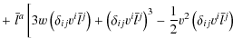
After long calculations and considering the IAU metric, the first term
on the righthand-side of this formula can be written as
![$\displaystyle \frac{\left(\bar{l}-\nu\right)_{\beta}\lambda_{\hat{a}}^{\beta}}{...
...ac{1}{c}\left[-v^{a}+\left(\delta_{ij}v^{i}\bar{l}^{j}\right)\bar{l}^{a}\right]$](/articles/aa/full_html/2010/01/aa12691-09/img105.png)
![$\displaystyle +\frac{1}{c^{2}}\left\{ w\bar{l}^{a}-\left(\delta_{ij}v^{i}\bar{l...
...elta_{ij}v^{i}\bar{l}^{j}\right)^{2}-\frac{1}{2}v^{2}\right]\bar{l}^{a}\right\}$](/articles/aa/full_html/2010/01/aa12691-09/img106.png)
![$\displaystyle \left.\left.+\left(\delta_{ij}v^{i}\bar{l}^{j}\right)^{3}-\frac{1...
...r{l}^{j}\right)\right]\right\}+\mathcal{O}\left(\frac{v^{4}}{c^{4}}\right)\cdot$](/articles/aa/full_html/2010/01/aa12691-09/img108.png)
The second term is zero since both
![$\displaystyle \frac{1}{2}\frac{\left(\bar{l}-\nu\right)_{i}\left(v^{i}/c\right)...
...}{c^{2}}\right]\frac{v^{a}}{c}+\mathcal{O}\left(\frac{v^{4}}{c^{4}}\right)\cdot$](/articles/aa/full_html/2010/01/aa12691-09/img111.png)
Finally, collecting all terms, we get
![$\displaystyle +\frac{1}{c^{2}}\left\{ w\bar{l}^{a}-\frac{1}{2}\left(\delta_{ij}...
...elta_{ij}v^{i}\bar{l}^{j}\right)^{2}-\frac{1}{2}v^{2}\right]\bar{l}^{a}\right\}$](/articles/aa/full_html/2010/01/aa12691-09/img113.png)
![$\displaystyle \left.\left.+w\left(\delta_{ij}v^{i}\bar{l}^{j}\right)\right]\right\} +\mathcal{O}\left(\frac{v^{4}}{c^{4}}\right)\cdot$](/articles/aa/full_html/2010/01/aa12691-09/img116.png)
3.3 Recasting to the GREM-like aberration
Expression (22) relates the observed direction cosines with
![]() .
The equivalent relation for the GREM observable is Eq. (B.6) where the aberration is expressed in terms of a vector
.
The equivalent relation for the GREM observable is Eq. (B.6) where the aberration is expressed in terms of a vector ![]() .
At first glance, it comes out that we cannot simply identify
.
At first glance, it comes out that we cannot simply identify
![]() with
with ![]() ,
since the last expression shows differences in terms up to the
,
since the last expression shows differences in terms up to the
![]() order! In particular, the appearance of the term
order! In particular, the appearance of the term
![]() and of different factors at the
and of different factors at the
![]() order cannot allow a straightforward comparison, as expected, of Eq. (22)
to the GREM vectorial one of Eq. (B.6).
Therefore, to compare formula (22) with GREM's formula (B.6) and find a relationship between
order cannot allow a straightforward comparison, as expected, of Eq. (22)
to the GREM vectorial one of Eq. (B.6).
Therefore, to compare formula (22) with GREM's formula (B.6) and find a relationship between ![]() and
and
![]() ,
we need to reduce the
,
we need to reduce the
![]() s to their coordinate Euclidean expressions.
s to their coordinate Euclidean expressions.
In GREM, ![]() represents the ``aberration-free'' coordinate
line of sight of the observed star at the position of the satellite
momentarily at rest. In RAMOD, as said,
represents the ``aberration-free'' coordinate
line of sight of the observed star at the position of the satellite
momentarily at rest. In RAMOD, as said,
![]() represents
the normalized local line-of-sight of the observed star
as seen by the local barycentric observer
represents
the normalized local line-of-sight of the observed star
as seen by the local barycentric observer ![]() .
In other words,
.
In other words,
![]() is a four-vector that fixes the
line of sight of an object with respect to the local BCRS. Do
is a four-vector that fixes the
line of sight of an object with respect to the local BCRS. Do ![]() and
and
![]() have a similar role in the
two approaches? From the physical point of view they have the same
meaning, as the observed ``aberration free'' direction
to the star. Let us start from the definition of
have a similar role in the
two approaches? From the physical point of view they have the same
meaning, as the observed ``aberration free'' direction
to the star. Let us start from the definition of ![]() in
GREM:
in
GREM:

|
where
On the other hand, using the definition of
|
and, from
Finally, from Eqs. (23) and (24) one has
namely, the spatial light direction, expressed in terms of its Euclidean counterpart at the satellite location in the gravitational field of the solar system. It is worth noticing that no terms of the order of
Combining Eq. (22) with (25) and
setting
![]() to ease the notation, we obtained
to ease the notation, we obtained
![$\displaystyle +\frac{1}{c^{2}}\left\{ -\frac{1}{2}\left(\vec{v}\cdot\vec{n}\rig...
...eft[\left(\vec{v}\cdot\vec{n}\right)^{2}-\frac{1}{2}v^{2}\right]n^{a}\right\} +$](/articles/aa/full_html/2010/01/aa12691-09/img136.png)
![$\displaystyle \left.+\left(\vec{v}\cdot\vec{n}\right)n^{a}\left[2w+\left(\vec{v...
...}-\frac{1}{2}v^{2}\right]\right\} +\mathcal{O}\left(\frac{v^{4}}{c^{4}}\right),$](/articles/aa/full_html/2010/01/aa12691-09/img138.png)
i.e. the righthand side of the aberration expression of RAMOD rewritten as in GREM.
Now we have to be certain that the lefthand side of
Eq. (26) can also be directly compared with GREM's
formula (B.6). Let us apply the tetrad property
![]() to the definition of
to the definition of
![]() and get
and get
Is there a relation between the direction cosines of this equation with the spatial components of the observed vector
In RAMOD, at the milli-arcsecond level, i.e. at (v/c)2, the rest-space of the local barycentric observer coincides globally with the spatial hyper-surfaces
that foliate the space-time and define the BCRS (de Felice et al. 2004).
At micro-arcsecond accuracy, instead, the vorticity cannot be neglected
and the geometry is affected by nondiagonal terms of the metric, meaning that
the
![]() hyper-surfaces do not coincide with the
rest-space of the local barycentric observer (de Felice et al. 2006).
Then, to be consistent, at each point of observation
we can only define a spatial direction measured by the local barycentric observer and
then associate it to the satellite measurements via the direction
cosines relative to the boosted attitude frame.
hyper-surfaces do not coincide with the
rest-space of the local barycentric observer (de Felice et al. 2006).
Then, to be consistent, at each point of observation
we can only define a spatial direction measured by the local barycentric observer and
then associate it to the satellite measurements via the direction
cosines relative to the boosted attitude frame.
The equivalence of the two coordinate systems thus holds if the origins of the
two reference systems coincide and only locally, i.e. in a sufficiently small
neighborhood, since the tetrads are not necessarily holonomic. Under
these hypotheses and from (B.1), one can state that
|
and it follows that
Therefore, using the local validity of Eq. (28) and considering that
![$\displaystyle \left.\frac{1}{2}\left[n^{a}\left(\vec{v}\cdot\vec{v}\right)-v^{a}\left(\vec{v}\cdot\vec{n}\right)\right]\right\} +$](/articles/aa/full_html/2010/01/aa12691-09/img152.png)
![$\displaystyle \left.\frac{1}{2}\left(\vec{v}\cdot\vec{n}\right)\left[n^{a}\left...
...cdot\vec{n}\right)\right]\right\} +\mathcal{O}\left(\frac{v^{4}}{c^{4}}\right).$](/articles/aa/full_html/2010/01/aa12691-09/img155.png)
Finally, from the relation
![$\displaystyle \left.+\frac{1}{2}\left[\vec{v}\times\left(\vec{n}\times\vec{v}\r...
...w\right]\left[\vec{n}\times\left(\vec{v}\times\vec{n}\right)\right]^{a} \right.$](/articles/aa/full_html/2010/01/aa12691-09/img158.png)
![$\displaystyle \left.+\frac{1}{2}\left(\vec{v}\cdot\vec{n}\right)\left[\vec{v}\t...
...s\vec{v}\right)\right]^{a}\right\} +\mathcal{O}\left(\frac{v^{4}}{c^{4}}\right)$](/articles/aa/full_html/2010/01/aa12691-09/img159.png)
which is formula (B.6) for the aberration in GREM-like model if we consider that
4 Conclusions
This paper compares two approaches within the context of relativistic astrometry, GREM and RAMOD, both suitable for modeling modern astrometric observations at micro-arcsecond accuracy. Because of the structure of GREM, the earliest stage of a theoretical comparison starts with the evaluation of the aberration ``effect'' in RAMOD.
This work presents a first analysis between two different methods in applying general relativity, the only theory of gravitation up to now, to astrometry. Understanding any difference and/or equivalence represents a valuable help to exploit the Gaia observations to their full extent and to validate data analysis in the new era of relativistic astrometry.
Indeed, the different mathematical structures of GREM and RAMOD hinder a straightforward comparison and call for a more in-depth analysis of the two models. While GREM favors the direct application of the coordinate approach since the beginning, RAMOD prefers, instead, to keep the meaning of the physical quantity as far as possible, i.e. to move to the coordinates once the condition equations are solved (namely the equations linking the measurements and astrometric unknowns). This implies a certain number of differences between the two derivations that have to be taken into account to avoid misinterpretations of parallel but different quantities. Up to now, we can distinguish the following differences in how the two models use: (i) the boundary conditions; (ii) the astrometric measurements; (iii) the attitude implementation; (iv) and the definition of the proper light direction.
Of crucial importance is point (i). The light signal arriving at the local BCRS along the spatial direction
![]() satisfies the RAMOD master equations, a set of nonlinear coupled
differential equations (de Felice et al. 2006). Therefore the
cosines (i.e. the astrometric measurements) taken as a function of
the local line of sight (the physical one), at the time of
observation, allow fixing the boundary conditions
needed to solve the master equations and determining
the star coordinates uniquely. However, since the direction cosines are expressed
in terms of the attitude, the mathematical characterization of the
attitude frame is essential for completing the boundary value
problem in the process of reconstructing the light trajectory. The
vector
satisfies the RAMOD master equations, a set of nonlinear coupled
differential equations (de Felice et al. 2006). Therefore the
cosines (i.e. the astrometric measurements) taken as a function of
the local line of sight (the physical one), at the time of
observation, allow fixing the boundary conditions
needed to solve the master equations and determining
the star coordinates uniquely. However, since the direction cosines are expressed
in terms of the attitude, the mathematical characterization of the
attitude frame is essential for completing the boundary value
problem in the process of reconstructing the light trajectory. The
vector ![]() in GREM, i.e. the ``aberration-free'' counterpart
of
in GREM, i.e. the ``aberration-free'' counterpart
of
![]() of RAMOD, is instead used to derive the aberration
effect (in a coordinate language), and there is no need to connect
it with a RAMOD-like boundary value problem.
of RAMOD, is instead used to derive the aberration
effect (in a coordinate language), and there is no need to connect
it with a RAMOD-like boundary value problem.
In RAMOD the direction cosines link the attitude of the satellite to the measurements, combining several reference frames useful to determine, as final task, the stellar coordinates: the BCRS (kinematically non-rotating global reference frame), the CoMRS (a local reference frame comoving with the satellite centre of mass), and the SRS (the attitude triad of the satellite). The coordinate transformations between BCRS/CoMRS/SRS come out naturally once the IAU conventions are adopted. A proof of this is given when we apply proper time formula (A.3) to get the relationship between the running time on board and the barycentric coordinate time (7). This is inside the conceptual framework of RAMOD, where the astrometric set-up allows one to trace the light ray back to the emitting star in a curved geometry, and it is not natural to disentangle each single effect. As for the solution of the geodesic equation, RAMOD defines a complete procedure to derive the satellite attitude that as input depends only on the specific terms of the metric that describes the addressed physical problem. GREM, instead, embeds the definition of its main reference system (BCRS) within the metric, consequently each further step depends on this choice. This includes all the subsequent transformations among the reference systems that are essential for extracting the GREM observable as a function of the astrometric unknowns. On the other side, the RAMOD directly implements in the solution of the astrometric problem the relativistic algorithms of the attitude frame, assuring its consistency with GR, since by definition the origin of the tetrad system follows the observer's world-line (i.e. the center of mass of the satellite in this case). The last comment explains items (ii) and (iii) and introduces item (iv).
Because physical quantities do not depend on the coordinates, the direction cosines are a powerful tool for comparing the astrometric relativistic models: their physical meaning allows us to correctly interpret the astrometric parameters in terms of coordinate quantities. This justified the conversion of the physical stellar proper direction of RAMOD into its analogous Euclidean coordinate counterpart, which ultimately leads to the derivation of a GREM-style aberration formula. Another point arises when the observables of RAMOD have to be identified with si, i.e. the components of the observed vector of GREM. This matching is admitted only if the origins of the boosted local BCRS tetrad in RAMOD and of the CoMRS in GREM coincide.
In conclusion, to what extent, then, is the process of star coordinate ``reconstruction'' consistent with General Relativity&Theory of Measurements? Solving the astrometric problem in practice means to compile an astrometric catalog with the same order of accuracy as the measurements. This paper shows not only that the two models give the same results, but also that particular care is needed in the interpretation of the observables and of the quantities that constitute the final catalog in order to avoid differences that already exist at the level of the aberration effect.
AcknowledgementsThe authors wish to thank Prof. Fernando de Felice and Dr. Mario G. Lattanzi for constant support and useful discussions. In particular, we thank the referee for his valuable comments and suggestions. This work is supported by the ASI grants COFIS and I/037/08/0.
Appendix A: Length and time measurements due to a space-time splitting
An observer ![]() carrying its laboratory is usually
represented as a world tube; in the case of a non-extended body, the world
tube can be restricted to a world line tracing the history of the observer's
barycenter in the given space-time. At any point P along the world line of
carrying its laboratory is usually
represented as a world tube; in the case of a non-extended body, the world
tube can be restricted to a world line tracing the history of the observer's
barycenter in the given space-time. At any point P along the world line of
![]() ,
and within a sufficiently small neighborhood, it is possible to
split the space-time into a one-dimensional space and a three-dimensional
one (de Felice & Clarke 1990), each space being endowed with its
own metric, respectively
,
and within a sufficiently small neighborhood, it is possible to
split the space-time into a one-dimensional space and a three-dimensional
one (de Felice & Clarke 1990), each space being endowed with its
own metric, respectively
![]() and
and
![]() .
Clearly,
.
Clearly,
The subspace with metric
As a consequence of Eq. (A.1), the invariant interval
between two events in space-time can be written as
![]() ,
from which we are able to extract the measurements of infinitesimal
spatial distances and time intervals taken by
,
from which we are able to extract the measurements of infinitesimal
spatial distances and time intervals taken by ![]() as, respectively,
as, respectively,
| (A.2) |
and
Appendix B: Stellar observed direction and stellar aberration in GREM-like approaches
The pN/pM approaches (Klioner 2003; Kopeikin & Mashhoon 2002; Kopeikin & Schäfer 1999)
transform the observed direction to the source (![]() )
into
the BCRS spatial coordinate direction of the light ray at the point
of observation with coordinates
)
into
the BCRS spatial coordinate direction of the light ray at the point
of observation with coordinates
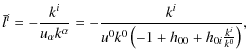
![]() (see Fig. B.1). Now, paraphrasing Klioner (2003),
the coordinate direction to the light source at
(see Fig. B.1). Now, paraphrasing Klioner (2003),
the coordinate direction to the light source at
![]() is defined by the four-vector
is defined by the four-vector
![]() ,
where
,
where
![]() ,
xi, and t are the BCRS coordinates. But the coordinate components
pi are not directly observable quantities; the observed vector
towards the light source is the four-vector
,
xi, and t are the BCRS coordinates. But the coordinate components
pi are not directly observable quantities; the observed vector
towards the light source is the four-vector
![]() ,
defined with respect to the local inertial frame of the observer.
In the local frame:
,
defined with respect to the local inertial frame of the observer.
In the local frame:

where
![\begin{figure}
\par\includegraphics[width=8cm]{12691fg2}
\end{figure}](/articles/aa/full_html/2010/01/aa12691-09/img179.png)
|
Figure B.1: The vectors representing the light direction in the pM/pN approaches inside the near-zone of the solar system. |
| Open with DEXTER | |
One can make Eq. (B.3) explicit by following the procedure reported in (Klioner & Kopeikin 1992) and adopting the IAU resolution B1.3 (Soffel et al. 2003). From the BCRS
and between the spatial coordinates as
![$\displaystyle \left[\delta_{j}^{i}+c^{-2}\left(\frac{1}{2}v^{i}v_{j}+qF_{j}^{i}(t)+D_{j}^{i}(t)\right)\right]R_{{\rm s}}^{j}$](/articles/aa/full_html/2010/01/aa12691-09/img188.png)
All the functions A, B, C, D are defined in Klioner & Kopeikin (1992) or in IAU resolutions, and
As reported in Klioner (2004), the attitude in GREM
(SRS) is obtained by applying an orthogonal rotation matrix
![]() to
to
![]() in Eq. (B.5). At this stage the role of the SRS is equivalent to that of the
in Eq. (B.5). At this stage the role of the SRS is equivalent to that of the
![]() s in Eq. (8).
s in Eq. (8).
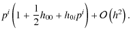
If one keeps all the terms up to the order of 1 micro-arcsecond,
the observed stellar direction si is transformed (in the CoMRS) into the unitary
``aberration-free'' direction
ni=pi/p (where
![]() ):
):
![$\displaystyle +c^{-2}\left\{ (\vec{n}\cdot\vec{v})\left[\vec{n}\times\left(\vec...
...ac{1}{2}\left[\vec{v}\times\left(\vec{n}\times\vec{v}\right)\right]^{i}\right\}$](/articles/aa/full_html/2010/01/aa12691-09/img198.png)
![$\displaystyle \left.+\frac{1}{2}\left(\vec{n}\cdot\vec{v}\right)\left[\vec{v}\t...
...left(\vec{n}\times\vec{v}\right)\right]^{i}\right\} +\mathcal{O}\left(4\right).$](/articles/aa/full_html/2010/01/aa12691-09/img200.png)
References
- Bastian, U. 2004, Reference System, Conventions and Notations for Gaia, Research Note GAIA-ARI-BAS-003, GAIA livelink [Google Scholar]
- Bini, D., Crosta, M. T., & de Felice, F. 2003, Class. Quantum Grav., 20, 4695 [Google Scholar]
- Crosta, M. T. 2003, Methods of Relativistic Astrometry for the analysis of astrometric data in the Solar System gravitational field, Ph.D. Thesis, Università di Padova, Centro Interdipartimentale di Studi e Attività Spaziali (CISAS) ``G. Colombo'' [Google Scholar]
- de Felice, F., & Clarke, C. J. S. 1990, Relativity on curved manifolds (Cambridge University Press) [Google Scholar]
- de Felice, F., & Preti, G. 2006, Class. Quantum Grav., 23, 5467 [Google Scholar]
- de Felice, F., Crosta, M. T., Vecchiato, A., Lattanzi, M. G., & Bucciarelli, B. 2004, ApJ, 607, 580 [NASA ADS] [CrossRef] [Google Scholar]
- de Felice, F., Vecchiato, A., Crosta, M. T., Bucciarelli, B., & Lattanzi, M. G. 2006, ApJ, 653, 1552 [NASA ADS] [CrossRef] [Google Scholar]
- Jantzen, R. T., Carini, P., & Bini, D. 1992, Ann. Phys., 215, 1 [Google Scholar]
- Klioner, S. A. 2003, AJ, 125, 1580 [Google Scholar]
- Klioner, S. A. 2004, Phys. Rev. D, 69, 124001 [NASA ADS] [CrossRef] [Google Scholar]
- Klioner, S. A., & Kopeikin, S. M. 1992, AJ, 104, 897 [NASA ADS] [CrossRef] [Google Scholar]
- Kopeikin, S. M., & Mashhoon, B. 2002, Phys. Rev. D, 65, 64025 [Google Scholar]
- Kopeikin, S. M., & Schäfer, G. 1999, Phys. Rev. D, 60, 124002 [NASA ADS] [CrossRef] [MathSciNet] [Google Scholar]
- Lattanzi, M. G., Drimmel, R., Gai, M., et al. 2006, Astrometric Verification Unit, Tech. rep., GAIA-C3-TN-INAF-ML-001-2 [Google Scholar]
- Misner, C. W., Thorne, K. S., & Wheeler, J. A. 1973, Gravitation, (San Francisco: W.H. Freeman and Co) [Google Scholar]
- Soffel, M., Klioner, S. A., Petit, G., et al. 2003, AJ, 126, 2687 [NASA ADS] [CrossRef] [Google Scholar]
- Turon, C., O'Flaherty, K. S., & Perryman, M. A. C. 2005, The Three-Dimensional Universe with Gaia [Google Scholar]
- Unwin, S. C., Shao, M., Tanner, A. M., et al. 2008, Publ. Astron. Soc. Pac., 120, 38 [Google Scholar]
Footnotes
- ... zone
![[*]](/icons/foot_motif.png)
- The near zone of a system of bound sources, which generates no stationary gravitational field, is defined as the region of space with a size comparable to the wavelength of the gravitational radiation emitted by that system.
- ... equations''
- These equations derive from the null geodesic with the appropriate projection onto the rest-space of the local barycentric observer (de Felice et al. 2004,2006).
- ... resolutions
- These resolutions are based on the pN approximation, which
is still
compatible with RAMOD, since the perturbation
 to
the Minkowskian metric in (1) can
be calculated
at any desired order of approximations in
to
the Minkowskian metric in (1) can
be calculated
at any desired order of approximations in  inside
the Solar System.
inside
the Solar System.
- ...
observation
- Also, each Eq. (8) is essential in RAMOD as it represents a boundary condition needed to uniquely solve the master equations.
All Figures
|
|
Figure 1:
The local observer |
| Open with DEXTER | |
| In the text | |
|
|
Figure B.1: The vectors representing the light direction in the pM/pN approaches inside the near-zone of the solar system. |
| Open with DEXTER | |
| In the text | |
Copyright ESO 2010
Current usage metrics show cumulative count of Article Views (full-text article views including HTML views, PDF and ePub downloads, according to the available data) and Abstracts Views on Vision4Press platform.
Data correspond to usage on the plateform after 2015. The current usage metrics is available 48-96 hours after online publication and is updated daily on week days.
Initial download of the metrics may take a while.