| Issue |
A&A
Volume 509, January 2010
|
|
|---|---|---|
| Article Number | A44 | |
| Number of page(s) | 13 | |
| Section | Interstellar and circumstellar matter | |
| DOI | https://doi.org/10.1051/0004-6361/200912594 | |
| Published online | 15 January 2010 | |
A method to determine distances to molecular clouds using near-IR photometry
G. Maheswar1,2 - C. W. Lee1 - H. C. Bhatt3 - S. V. Mallik3 - S. Dib4,5
1 - Korea Astronomy and Space Science Institute, 61-1, Hwaam-dong, Yuseong-gu, Daejeon 305-348, Republic of Korea
2 -
Aryabhatta Research Institute of Observational Sciences, Manora Peak, Nainital 263 129, India
3 -
Indian Institute of Astrophysics, Koramangala, Bangalore 560 034, India
4 -
Service d'Astrophysique, DSM/Irfu, CEA/Saclay, 91191 Gif-sur-Yvette Cedex, France
5 -
Lebanese University, Faculty of Sciences, Department of Physics, El-Hadath, Beirut, Lebanon
Received 29 May 2009 / Accepted 23 September 2009
Abstract
Aims. We aim to develop a method to determine distances to molecular clouds using JHK near-infrared photometry.
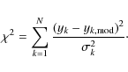
Methods. The method is based on a technique that aids spectral
classification of stars lying towards the fields containing the clouds
into main sequence and giants. In this technique, the observed (J-H) and (
![]() )
colours are dereddened simultaneously using trial values of AV
and a normal interstellar extinction law. The best fit of the
dereddened colours to the intrinsic colours giving a minimum value of
)
colours are dereddened simultaneously using trial values of AV
and a normal interstellar extinction law. The best fit of the
dereddened colours to the intrinsic colours giving a minimum value of ![]() then yields the corresponding spectral type and AV for the star. The main sequence stars, thus classified, are then utilized in an AV versus distance plot to bracket the cloud distances.
then yields the corresponding spectral type and AV for the star. The main sequence stars, thus classified, are then utilized in an AV versus distance plot to bracket the cloud distances.
Results. We applied the method to four clouds, L1517, Chamaeleon I, Lupus 3 and NGC 7023 and estimated their distances as ![]() ,
,
![]() ,
,
![]() and
and ![]() pc respectively, which are in good agreement with the previous distance estimations available in the literature.
pc respectively, which are in good agreement with the previous distance estimations available in the literature.
Key words: dust, extinction - ISM: clouds - stars: distances - infrared: ISM
1 Introduction
The knowledge of the distance to interstellar clouds which are either isolated or associated with large complexes, star forming or starless, is important to provide observational constraints to the properties of clouds and pre-main sequence (PMS) stars (e.g., Yun & Clemens 1990; Clemens et al. 1991; Kauffmann et al. 2008). However, distances to many of these clouds, especially those that are isolated, are highly uncertain (in some cases, by a factor of 2, see Hilton & Lahulla 1995).
In recent years, successful efforts have been made to estimate distances to large complexes using a number of methods. For example, combining extinction maps from the Two Micron All Sky Survey (2MASS) with Hipparcos and Tycho parallaxes, Lombardi et al. (2008) estimated accurate distances to the Ophiuchus and Lupus dark cloud complexes; the Hipparcos parallax measurements and B-band polarimetry were utilized by Alves & Franco (2007) to estimate the distance of the Pipe nebula. Using multi-epoch very long baseline array (VLBA) observations of a number of young stellar objects (YSOs), Loinard et al. (2007) measured the trigonometric parallaxes and hence distances with a precision of about 1-4% (Loinard et al. 2007, 2008). The distances to the parent clouds that harbour these YSOs are also constrained with similar precision.
However, it is difficult to establish distances to isolated clouds devoid of low-mass YSOs and primary indicators such as ionizing stars or reflection nebulae. Distances to these clouds can be assigned through their association (in position-velocity space) with nearby larger molecular clouds (e.g., Kauffmann et al. 2008) which have their distances determined through the abovementioned methods. The traditional ways of determining distances to isolated clouds utilize the star count method (Bok & Bok 1941) or Wolf diagrams (Wolf 1923), which is limited due to its dependence on the questionable extrapolation of luminosity functions. Additional methods of assigning distances to small dark clouds have involved bracketing the cloud distance by using spectroscopic distances to stars (Hobbs et al. 1986) and using the equivalent widths of interstellar Ca II H and K lines of stars close in front of and behind the cloud (Megier et al. 2005). However, spectroscopy of a large number of stars projected on a cloud is extremely demanding in terms of telescope time. Because of the absence of nearby associated large molecular clouds or stellar spectroscopic data, distances of most of the isolated small clouds remain unknown.
Distances to clouds can be determined by bracketing them using
spectral classification of stars projected on to the cloud purely by
photometry carried out in the Vilnius photometric system (Straizys 1991; Straizys et al. 1992). The distance and reddening for individual stars can also be obtained using the very well calibrated Stromgren
![]() intermediate-narrow- band photometric system. The physical parameters
of stars thus obtained are utilized to bracket the cloud distances
(e.g., Nielsen et al. 2000; Franco 2002). Another innovative method was developed by Peterson & Clemens (1998)
by identifying M dwarfs lying both in front of and behind the cloud.
The reddening and spectral types of these M dwarfs were determined from
photometry alone due to their conspicuous position in the (V-I) versus (B-V) colour-colour (CC) diagram. The optical V, R, I and near-IR (NIR) J, H and K 2MASS colours were utilized by Maheswar et al. (2004, 2006) to bracket cloud distances, again by spectral classification of stars projected on to them from photometry alone.
intermediate-narrow- band photometric system. The physical parameters
of stars thus obtained are utilized to bracket the cloud distances
(e.g., Nielsen et al. 2000; Franco 2002). Another innovative method was developed by Peterson & Clemens (1998)
by identifying M dwarfs lying both in front of and behind the cloud.
The reddening and spectral types of these M dwarfs were determined from
photometry alone due to their conspicuous position in the (V-I) versus (B-V) colour-colour (CC) diagram. The optical V, R, I and near-IR (NIR) J, H and K 2MASS colours were utilized by Maheswar et al. (2004, 2006) to bracket cloud distances, again by spectral classification of stars projected on to them from photometry alone.
The enormous NIR dataset provided by the 2MASS (Kleinmann et al. 1994)
was extensively used by several authors, mainly (a) to discriminate
between normal stars and stars with significant NIR emission from
circumstellar material (e.g., Itoh et al. 1996) and (b) to map the extinction in dense molecular clouds (Cambrésy et al. 2002; Lombardi et al. 2006). Dutra et al. (2003) built an AK extinction map of a
![]() field towards the Galactic centre using 2MASS J and
field towards the Galactic centre using 2MASS J and ![]() magnitudes. They utilized the upper giant branch of colour-magnitude
diagrams and their dereddened mean locus built from previous studies of
bulge fields to estimate the extinction. In this work, we present a
method by which distances to molecular clouds are estimated using (J-H), (
magnitudes. They utilized the upper giant branch of colour-magnitude
diagrams and their dereddened mean locus built from previous studies of
bulge fields to estimate the extinction. In this work, we present a
method by which distances to molecular clouds are estimated using (J-H), (
![]() )
colour indices of the main sequence stars in the spectral range from A0
to K7. The technique is based on a methodology that provides spectral
classification of stars projected on to the fields containing the cloud
into main sequence and giants by simultaneously dereddening the (J-H) and (
)
colour indices of the main sequence stars in the spectral range from A0
to K7. The technique is based on a methodology that provides spectral
classification of stars projected on to the fields containing the cloud
into main sequence and giants by simultaneously dereddening the (J-H) and (
![]() )
observed colours using trial values of AV and a normal interstellar extinction law. The main sequence stars are then utilized in an AV vs.
distance (d) plot to bracket the cloud distances. In Sect. 2 we describe the method for finding the spectral type, AV, and distances to the molecular clouds using NIR data from the 2MASS. The uncertainties involved in the determination of the AV values and the distances from the method are also discussed in this section. In Sect. 3 we describe the criteria used to extract the data from the 2MASS database. In Sect. 4
we apply our technique to four clouds, L1517, Chamaeleon I, Lupus and
NGC 7023. We discuss the method in determining distances to dark
molecular clouds in Sect. 5. Finally, we conclude the paper by summarizing the results obtained in Sect. 6.
)
observed colours using trial values of AV and a normal interstellar extinction law. The main sequence stars are then utilized in an AV vs.
distance (d) plot to bracket the cloud distances. In Sect. 2 we describe the method for finding the spectral type, AV, and distances to the molecular clouds using NIR data from the 2MASS. The uncertainties involved in the determination of the AV values and the distances from the method are also discussed in this section. In Sect. 3 we describe the criteria used to extract the data from the 2MASS database. In Sect. 4
we apply our technique to four clouds, L1517, Chamaeleon I, Lupus and
NGC 7023. We discuss the method in determining distances to dark
molecular clouds in Sect. 5. Finally, we conclude the paper by summarizing the results obtained in Sect. 6.
2 The method
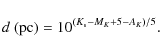
The photometric distance d to a star is estimated using the distance equation
where V, MV, AV, K, MK, and AK are the apparent magnitude, absolute magnitude and extinction in V and K filters respectively. Spectral type and luminosity class information are needed to determine both absolute magnitude of a star and the extinction suffered by it due to interstellar dust in the line of sight. Spectral type and luminosity class also determine the various colours of a star. Therefore, in principle, one could determine the spectral type and the luminosity of a star from its observed colours provided the extinction is zero. In practice, observed colours are reddened due to interstellar extinction, which is wavelength-dependent. By assuming a value for AV and an extinction law one could estimate the colour excesses and correct the observed colours to find the intrinsic colours of the stars and hence their spectral types.
2.1 The (J - H), (H - K )
intrinsic colours
)
intrinsic colours
In Fig. 1, we present the (J-H), (
![]() )
CC diagram. The solid line represents locations of unreddened main
sequence stars. Usually the unreddened colours of different spectral
types and luminosity classes in the 2MASS system are obtained from
Koornneef (1983) or Bessell & Brett (1988) using the transformation equations given by Carpenter (2001).
We produced the intrinsic colours of the main sequence stars in the
spectral range from A0 to K7 in the 2MASS system directly from the
observations by selecting stars from the All-sky Compiled Catalogue of 2.5 million stars
(Kharchenko 2001) catalogue with known spectral types and which lie
within 100 pc (estimated from their Hipparcos parallax measurements)
from us. The mean values of (J-H) and (
)
CC diagram. The solid line represents locations of unreddened main
sequence stars. Usually the unreddened colours of different spectral
types and luminosity classes in the 2MASS system are obtained from
Koornneef (1983) or Bessell & Brett (1988) using the transformation equations given by Carpenter (2001).
We produced the intrinsic colours of the main sequence stars in the
spectral range from A0 to K7 in the 2MASS system directly from the
observations by selecting stars from the All-sky Compiled Catalogue of 2.5 million stars
(Kharchenko 2001) catalogue with known spectral types and which lie
within 100 pc (estimated from their Hipparcos parallax measurements)
from us. The mean values of (J-H) and (
![]() )
colours produced are listed in Cols. 3 and 4 of Table 1,
respectively. The standard deviations and the number of stars used to
evaluate the colours are given in Cols. 5, 6 and 7. The MK values obtained from MV and (V-K) from Cox (2000)
are listed in Col. 2. The intrinsic colors of the main sequence
stars and giants in the spectral range K8 to M6 were converted from
Bessell & Brett (1988) to the 2MASS system using the transformation equations given by Carpenter (2001).
We interpolated the intrinsic colour indices of normal main sequence
stars and giants to generate values with a 0.5 spectral sub-type
interval.
)
colours produced are listed in Cols. 3 and 4 of Table 1,
respectively. The standard deviations and the number of stars used to
evaluate the colours are given in Cols. 5, 6 and 7. The MK values obtained from MV and (V-K) from Cox (2000)
are listed in Col. 2. The intrinsic colors of the main sequence
stars and giants in the spectral range K8 to M6 were converted from
Bessell & Brett (1988) to the 2MASS system using the transformation equations given by Carpenter (2001).
We interpolated the intrinsic colour indices of normal main sequence
stars and giants to generate values with a 0.5 spectral sub-type
interval.
![\begin{figure}
\par\includegraphics[height=8.1cm,width=8.3cm,clip]{12594fg1.ps}
\end{figure}](/articles/aa/full_html/2010/01/aa12594-09/img33.png)
|
Figure 1:
The (J-H) vs. (
|
| Open with DEXTER | |
Table 1:
The estimated
![]() and
and
![]() intrinsic colours for main sequence stars.
intrinsic colours for main sequence stars.
The locations of stars with various spectral types are identified and marked in Fig. 1. The dashed line is drawn parallel to the Rieke & Lebofsky (1985) interstellar reddening vector. An unreddened main sequence normal star would move parallel to the reddening vector because of the extinction due to the interstellar dust along the line of sight. But as stars of spectral range A0 to K7 move parallel to the reddening vector, it would be difficult to differentiate between reddened stars in the spectral range A0 to K7 from unreddened M-type normal stars because the M-type stars lie across these vectors. However, for the stars lying below M-type stars loci, it is certain that they are reddened or unreddened normal stars in the spectral range A0 to K7. The stars that occupy the region enclosed by the main sequence star loci (i.e., from A0-K7), reddening vector for an A0 type star and below M-type loci were utilized in this work to determine distances to the dark clouds.
2.2 Spectral types and A from near-IR colours
We used a procedure known as ``photometric quantification'', which
is the procedure of inferring spectral type, and hence absolute
magnitude and intrinsic colours of normal main sequence stars and
giants from NIR photometry. In this method, stars with their
![]()
![]() were chosen from the fields containing the cloud. Then a set of dereddened colours [
were chosen from the fields containing the cloud. Then a set of dereddened colours [
![]() and
and
![]() ]
was produced for each star from their observed colours [(J-H) and (
]
was produced for each star from their observed colours [(J-H) and (
![]() )] by using trial values of AV and the Rieke & Lebofsky (1985)
)] by using trial values of AV and the Rieke & Lebofsky (1985)![]() extinction law in the equations
extinction law in the equations
the trial values of AV were chosen in the range 0-10 mag with an interval of 0.01 mag, though it is evident from Fig. 1 that the maximum extinction that could be traced by this method is limited to
But while the uncertainties in the magnitudes in J, H and
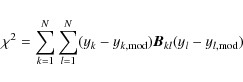
where
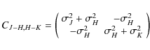
|
(6) |
with the off-diagonal elements having non-zero values unlike in the case of uncorrelated uncertainties. The expected value of
![\begin{figure}
\par\includegraphics[height=8.3cm,width=8.8cm,clip]{12594fg2.ps}
\end{figure}](/articles/aa/full_html/2010/01/aa12594-09/img54.png)
|
Figure 2:
The relation between the uncertainties in (J-H) and (
|
| Open with DEXTER | |
The whole procedure is illustrated in Fig. 1
where we plot the NIR-CC diagram for stars chosen from an arbitrary
location on the sky. The arrows are drawn from the observed data points
to the corresponding dereddened colours estimated using our method. The
maximum extinction values that can be measured using the method are
those for A0V type stars (![]() 4 mag). The extinction traced by stars falls as we move towards more late type stars.
4 mag). The extinction traced by stars falls as we move towards more late type stars.
2.3 Distances to dark molecular clouds
Once the spectral type and the AV of the stars are known, we calculate their distances using the equation
|
(7) |
We excluded the stars classified as giants because of the large uncertainty in their absolute magnitudes. The distance at which the extinction of the stars showed a sudden increase in an AV vs. d plot was considered as the distance to the cloud.
2.4 Limitations and uncertainties
The uncertainty in the determination of distances to the clouds depends
on the uncertainty in the estimation of distances to the individual
stars which is given by
![\begin{displaymath}\sigma_{d} =\sqrt[]{(\sigma_{K_{\rm s}}^2+\sigma_{M_{K}}^2+\sigma_{A_{K}}^2)\times(d/2.17)^2}~~~~~~~~~({\rm pc})\\
\end{displaymath}](/articles/aa/full_html/2010/01/aa12594-09/img56.png)
where
We allowed a maximum photometric uncertainty![]() of 0.035 mag for the sources in the J, H, and
of 0.035 mag for the sources in the J, H, and ![]() bands.
The uncertainty in the absolute magnitudes or the spectral types
determined from our method was evaluated by applying it to stars with
known distances from Hipparcos taken from the catalogue by Kharchenko
(2001). We used stars located within 100 pc of the Sun so that the
effect of the extinction could be neglected. Then, Eq. (8) applied to the Hipparcos stars becomes
bands.
The uncertainty in the absolute magnitudes or the spectral types
determined from our method was evaluated by applying it to stars with
known distances from Hipparcos taken from the catalogue by Kharchenko
(2001). We used stars located within 100 pc of the Sun so that the
effect of the extinction could be neglected. Then, Eq. (8) applied to the Hipparcos stars becomes
![\begin{displaymath}\sigma_{d_{\rm H}}=\sqrt[]{(\sigma_{K_{\rm s}}^2+\sigma_{M_{K}}^2)\times(d/2.17)^2}
.
\end{displaymath}](/articles/aa/full_html/2010/01/aa12594-09/img61.png)
In Fig. 3, we show histograms of the difference (
![\begin{figure}
\par\includegraphics[width=8cm,clip]{12594fg3.ps}\vspace*{-2mm}
\end{figure}](/articles/aa/full_html/2010/01/aa12594-09/img71.png)
|
Figure 3:
a) Histogram of the difference between the distances of the
main sequence stars from our method and those from the Hipparcos
parallax measurements with
|
| Open with DEXTER | |
The AV values obtained for the stars from our method are those which when used to deredden the observed colours (in Eqs. (2) and (3)) gave minimum values of ![]() .
Therefore the AV values obtained are equivalent to the average value of AV calculated using the individual colours, i.e.,
.
Therefore the AV values obtained are equivalent to the average value of AV calculated using the individual colours, i.e.,
![]() .
Since the colours are found to be correlated, the expression for evaluating the uncertainty in AV is
.
Since the colours are found to be correlated, the expression for evaluating the uncertainty in AV is
![\begin{displaymath}\sigma(A_{V}) \!=\!\sqrt[]{4.7^2 \cdot \sigma_{JH}^2+7.9^2 \c...
..._{HK_{\rm s}}^2\!+\!2\times37\!\times\! {\rm cov}(JH, HK)}
\\
\end{displaymath}](/articles/aa/full_html/2010/01/aa12594-09/img73.png)
where
The true spectral type and the AV of the stars evaluated from our method directly depend on the reddening or extinction law that we adopt. Unlike in visual and UV wavelengths where the extinction law is known to vary along different sight lines in the Galaxy (Mathis 1990), the similarity in the wavelength dependence of extinction for very different line of sights passing through different environments like the giant H II region (RCW 49) and the ``field'' region (Indebetouw et al. 2005) suggests that the extinction law is almost universal in the near-IR regime considered here. Consequently, the observed colours can be corrected for the reddening to determine the spectral type of the stars using a standard extinction law. But any deviation of the reddening law from the standard extinction law towards the region containing the clouds could introduce a systematic error in the distances estimated using our method.
3.4 Determination of cloud distance from A-distance plot
![\begin{figure}
\par\includegraphics[height=7cm,width=8.5cm,clip]{12594fg4.ps}
\end{figure}](/articles/aa/full_html/2010/01/aa12594-09/img77.png)
|
Figure 4: Procedure used to determine distances to the clouds from an AV vs. d as described in Sect. 2.5. The extinction of stars in situations with and without the presence of a cloud in the field-of-view of a region is represented by open and closed circles. The mean value of extinction in each distance bin in case of with and without cloud is shown by red and blue solid lines, respectively. |
| Open with DEXTER | |
The presence of an interstellar cloud should reveal itself by a sudden onset of extinction at a certain distance. If the cloud is isolated and is the first interstellar feature encountered, the excess should almost equal to zero in front of the cloud (e.g., Straizys et al. 1992; Whittet et al. 1997; Knude & Høg 1998; Alves & Franco 2006; Lombardi et al. 2008). In this technique, the distance to the cloud is typically estimated from the first star that shows a significant reddening. The estimated distance is thus regarded as an upper limit due to the lack of information on the closeness of this background star to the cloud. In our method, because we used a relatively large number of stars projected towards the cloud, we often found an almost continuous distribution of stars with high extinction beyond a certain distance.
In Fig. 4 we show a schematic figure of an AV vs. d
plot for an ideal situation along a line of sight through the Galactic
plane. The extinction suffered by the stars increases as a function of
their distance (typically, ![]() 1.8 mag kpc-1 is the value considered for the standard mean rate of diffuse-ISM extinction in the Galactic plane near the Sun, Whittet 1992) is represented by filled circles. If we group the stars in distance bins and calculate the mean AV of the stars for each bin, they would follow the blue curve as shown in Fig. 4.
The open circles represent the situation when a cloud of constant
extinction is introduced at a certain distance in the field-of-view.
Now, the mean AV of the stars in the bins
behind the cloud would show a jump equal to the extinction introduced
by the cloud (red curve). The distance at which the first sudden
increase in the mean AV occurs could be considered as the distance to the cloud (marked by the vertical dashed line in Fig. 4).
1.8 mag kpc-1 is the value considered for the standard mean rate of diffuse-ISM extinction in the Galactic plane near the Sun, Whittet 1992) is represented by filled circles. If we group the stars in distance bins and calculate the mean AV of the stars for each bin, they would follow the blue curve as shown in Fig. 4.
The open circles represent the situation when a cloud of constant
extinction is introduced at a certain distance in the field-of-view.
Now, the mean AV of the stars in the bins
behind the cloud would show a jump equal to the extinction introduced
by the cloud (red curve). The distance at which the first sudden
increase in the mean AV occurs could be considered as the distance to the cloud (marked by the vertical dashed line in Fig. 4).
In real cases, we grouped the stars into distance bins of
![]() .
The centers of each bin were separated by the half of the bin width.
Because there exist very few stars at smaller distances, the mean of
the distances and the AV
of the stars in each bin were calculated by taking 1000 pc as the
initial point and proceeding towards smaller distances (see Fig. 17).
The mean distance of the stars in the bin at which a significant drop
in the mean of the extinction occurred was taken as the distance to the
cloud and the average of the uncertainty in the distances of the stars
in that bin was taken as the final uncertainty in our distance
determination for the clouds. For all the clouds studied in this work,
the vertical dashed lines in AV vs. d plots, used to mark the cloud distances, were drawn at distances deduced from the above procedure (see Fig. 17). The error in the mean values of AV were calculated using the expression
.
The centers of each bin were separated by the half of the bin width.
Because there exist very few stars at smaller distances, the mean of
the distances and the AV
of the stars in each bin were calculated by taking 1000 pc as the
initial point and proceeding towards smaller distances (see Fig. 17).
The mean distance of the stars in the bin at which a significant drop
in the mean of the extinction occurred was taken as the distance to the
cloud and the average of the uncertainty in the distances of the stars
in that bin was taken as the final uncertainty in our distance
determination for the clouds. For all the clouds studied in this work,
the vertical dashed lines in AV vs. d plots, used to mark the cloud distances, were drawn at distances deduced from the above procedure (see Fig. 17). The error in the mean values of AV were calculated using the expression
![]() where N is the number of stars in each bin.
where N is the number of stars in each bin.
3 The data
We extracted J, H and ![]() magnitudes of stars from the 2MASS All-Sky Catalog of Point Sources
(Cutri et al. 2003) that satisfied the following criteria,
magnitudes of stars from the 2MASS All-Sky Catalog of Point Sources
(Cutri et al. 2003) that satisfied the following criteria,
- 1.
- photometric uncertainty
 in all the three filters;
- 2.
- photometric quality flag of ``AAA'' in all the three filters, i.e., signal-to-noise ratio (SNR) >10.
4 Distances to the molecular clouds L1517, Chamaeleon I, Lupus 3 and NGC 7023
We applied our method to four clouds, L1517, Chamaeleon I (Cha I), Lupus 3 (Lup 3) and NGC 7023, to determine distances to them. We preferred these four regions as they are structurally less complex and have had their distances estimated previously. Also, these clouds harbour stars (inferred from the associated nebulosity) for which distances from the Hipparcos parallax measurements are available (van den Ancker et al. 1998; Bertout et al. 1999), which would help constrain the parent cloud distances better. In Table 2, we list the distances to them compiled from the literature. The central coordinates, total number of stars selected and the number of stars classified as dwarfs and that were used to determine distances to the individual clouds are listed in Cols. 2-5 of Table 3 respectively.
Table 2: Distances to the clouds L1517, Cha I, Lup 3 and NGC 7023 compiled from the literature.
Table 3: The central coordinates, the number of stars selected from each field and the stars classified as dwarfs.
4.1 L 1517
![\begin{figure}
\par\includegraphics[width=8.7cm,clip]{12594fg5.ps}
\end{figure}](/articles/aa/full_html/2010/01/aa12594-09/img91.png)
|
Figure 5:
The
|
| Open with DEXTER | |
![\begin{figure}
\par\includegraphics[height=8.8cm,width=8.8cm,clip]{12594fg6.ps}
\end{figure}](/articles/aa/full_html/2010/01/aa12594-09/img92.png)
|
Figure 6:
The NIR-CC diagrams for the stars selected from the four fields
containing L1517 are shown. The dots represent all the stars in a given
field with photometric errors |
| Open with DEXTER | |
![\begin{figure}
\par\includegraphics[width=9cm,clip]{12594fg7.ps}
\end{figure}](/articles/aa/full_html/2010/01/aa12594-09/img93.png)
|
Figure 7:
The AV vs. d
plot for all the stars obtained from the fields F1-F4 combined towards
L1517. The dashed vertical line is drawn at 167 pc inferred from the
procedure described in the Sect. 2.5. The solid curve represents the increase in the extinction towards the Galactic latitude of
|
| Open with DEXTER | |
![\begin{figure}
\par\includegraphics[width=8.5cm,clip]{12594fg8.ps}
\end{figure}](/articles/aa/full_html/2010/01/aa12594-09/img94.png)
|
Figure 8:
The AV vs. d
plots for the stars from the fields F1-F4 towards L1517. The dashed
vertical line is drawn at 167 pc inferred from the procedure described
in Sect. 2.5. The solid curve represents the increase in the extinction towards the Galactic latitude of
|
| Open with DEXTER | |
In Fig. 5 we present the
![]() high resolution extinction map
high resolution extinction map![]() produced by Dobashi et al. (2005) of the region containing L1517.
The contours are drawn at 0.5, 1.0, 1.5 and 2 mag levels. The
Herbig Ae star, AB Aur (Herbig 1960; The et al. 1994), associated
with the reflection nebulosity, GN 04.52.5.02 (Magakian 2003), is
identified in Fig. 5.
produced by Dobashi et al. (2005) of the region containing L1517.
The contours are drawn at 0.5, 1.0, 1.5 and 2 mag levels. The
Herbig Ae star, AB Aur (Herbig 1960; The et al. 1994), associated
with the reflection nebulosity, GN 04.52.5.02 (Magakian 2003), is
identified in Fig. 5.
Some of the stars classified as main sequence by our method could
actually be giants. Such erroneous classifications could lead to an
underestimation of their distances which could create confusion with
the real increase in the extinction due to the presence of a cloud.
This problem could be circumvented if we divide a large field,
containing the cloud, into small sub-fields. While the rise in the
extinction due to the presence of a cloud should occur almost at the
same distance in all the fields, if the whole cloud is located at the
same distance, the wrongly classified stars in the sub-fields would
show high extinction not at the same but at random distances. We
divided the region containing L1517 into four fields as shown in Fig. 5. Each field is of
![]() in area. The central coordinates, the number of stars selected after applying all the selection criteria (
in area. The central coordinates, the number of stars selected after applying all the selection criteria (
![]() ,
SNR>10, and
,
SNR>10, and
![]() )
and the number of stars classified as dwarfs by our method from each field are listed in Table 3. In Fig. 6 we show the NIR-CC diagrams for the stars selected from F1-F4. The stars with their photometric errors
)
and the number of stars classified as dwarfs by our method from each field are listed in Table 3. In Fig. 6 we show the NIR-CC diagrams for the stars selected from F1-F4. The stars with their photometric errors ![]() 0.035 mag in J, H, and
0.035 mag in J, H, and ![]() bands are shown as dots and among them the stars with
bands are shown as dots and among them the stars with
![]() are identified by open circles. The stars classified as dwarfs using
our method are identified by filled circles (in white) in Fig. 5.
It can be noticed that very few sources are selected towards the high
extinction regions due to our data selection criteria discussed in
Sect. 3.
are identified by open circles. The stars classified as dwarfs using
our method are identified by filled circles (in white) in Fig. 5.
It can be noticed that very few sources are selected towards the high
extinction regions due to our data selection criteria discussed in
Sect. 3.
In Fig. 7 we show the AV vs. d
plot for the stars from all the fields combined. The solid curve shows
the increase in the extinction towards the Galactic latitude
![]() as a function of distance, produced using the expressions given by Bahcall & Soneira (1980,
BS80, hereafter). Clearly, the stars with high extinction located
beyond 167 pc, marked by the vertical dashed line (drawn using the
procedure described in the Sect. 2.5, see Fig. 17), are distributed almost continuously. There exists one star with AV>1 mag at a distance closer than 167 pc. The AV vs. d plots for the stars from the individual fields F1-F4 are shown in Fig. 8.
The stars showing high extinction at 167 pc are located in the fields
F1 and F4, which contain the major parts of the cloud. The high
extinction star closer than 167 pc in the field F4 is identified using
filled star symbol in Fig. 5. Because the star is projected within the cloud boundary, it is likely to be a misclassified source located behind the cloud.
as a function of distance, produced using the expressions given by Bahcall & Soneira (1980,
BS80, hereafter). Clearly, the stars with high extinction located
beyond 167 pc, marked by the vertical dashed line (drawn using the
procedure described in the Sect. 2.5, see Fig. 17), are distributed almost continuously. There exists one star with AV>1 mag at a distance closer than 167 pc. The AV vs. d plots for the stars from the individual fields F1-F4 are shown in Fig. 8.
The stars showing high extinction at 167 pc are located in the fields
F1 and F4, which contain the major parts of the cloud. The high
extinction star closer than 167 pc in the field F4 is identified using
filled star symbol in Fig. 5. Because the star is projected within the cloud boundary, it is likely to be a misclassified source located behind the cloud.
The distances to the molecular clouds in the Taurus-Auriga complex is
considered as 140 pc based on the star count, photometric distances of
reflecting nebulae and reddening versus distance diagrams of the field
stars towards the entire complex. But the most reliable estimation of
the distance to L1517 is based on the Hipparcos parallax measurements
of the two stars, AB Aur and SU Aur, found associated with the cloud.
The Hipparcos distances to these stars are
144 +23-17 and
152+63-34 respectively. The distance of ![]() pc to L1517 determined from our method are found to be in good
agreement with the distances of AB Aur and SU Aur within the
uncertainties.
pc to L1517 determined from our method are found to be in good
agreement with the distances of AB Aur and SU Aur within the
uncertainties.
4.2 Chamaeleon 1
![\begin{figure}
\par\includegraphics[width=8.5cm,clip]{12594fg9.ps}
\end{figure}](/articles/aa/full_html/2010/01/aa12594-09/img100.png)
|
Figure 9:
The
|
| Open with DEXTER | |
![\begin{figure}
\par\includegraphics[height=7cm,width=8.5cm,clip]{12594f10.ps}
\end{figure}](/articles/aa/full_html/2010/01/aa12594-09/img101.png)
|
Figure 10:
The AV vs. d
plot for the stars from all the fields (F1-F6) of Cha I combined. The
vertical dashed line is drawn at 151 pc inferred from the procedure
described in Sect. 2.5. The vertical dotted line indicates the distance of a possible foreground dust layer at |
| Open with DEXTER | |
![\begin{figure}
\par\includegraphics[width=7.8cm,clip]{12594f11.ps}
\end{figure}](/articles/aa/full_html/2010/01/aa12594-09/img102.png)
|
Figure 11:
The AV vs. d
plot for stars in the fields F1-F6 selected towards Cha I. The dashed
vertical line is at 151 pc inferred from the procedure described in
Sect. 2.5. The dotted
vertical line is drawn at 128 pc. The solid curve represents the
increase in the extinction towards the Galactic latitude of
|
| Open with DEXTER | |
The region containing the cloud Cha I is shown in the
![]() extinction map produced by Dobashi et al. (2005) in Fig. 9. The contours are drawn at 0.5, 1.0, 1.5 and 2.0 mag levels. Since the cloud is extended over a region of about
extinction map produced by Dobashi et al. (2005) in Fig. 9. The contours are drawn at 0.5, 1.0, 1.5 and 2.0 mag levels. Since the cloud is extended over a region of about
![]() area, we divided the whole region into six sub-fields of
area, we divided the whole region into six sub-fields of
![]() each as identified in Fig. 9. The central coordinates, total number of stars selected after applying all the selection criteria (
each as identified in Fig. 9. The central coordinates, total number of stars selected after applying all the selection criteria (
![]() ,
SNR>10, and (
,
SNR>10, and (
![]() )
and the number of stars classified as dwarfs using our method in each field are listed in Table 3. Stars classified as dwarfs are identified in Fig. 9 using filled circles. Here too we find very few sources towards the high extinction regions.
)
and the number of stars classified as dwarfs using our method in each field are listed in Table 3. Stars classified as dwarfs are identified in Fig. 9 using filled circles. Here too we find very few sources towards the high extinction regions.
In Fig. 10, we show the AV vs. d
plot for stars from all the fields combined. The solid curve represents
the increase in the extinction towards the Galactic latitude of
![]() as a function of distance produced using the expressions given by BS80. Using the procedure described in Sect. 2.5, we found a drop in the extinction at 151 pc (marked by the vertical dashed line in Fig. 10) as shown in Fig. 17. But the drop in the extinction at 151 pc was not as conspicuous as was observed towards L1517. Three stars with
as a function of distance produced using the expressions given by BS80. Using the procedure described in Sect. 2.5, we found a drop in the extinction at 151 pc (marked by the vertical dashed line in Fig. 10) as shown in Fig. 17. But the drop in the extinction at 151 pc was not as conspicuous as was observed towards L1517. Three stars with
![]() were found to be located closer than 151 pc (identified in Fig. 9 using filled star symbols). We noticed another drop in the extinction at 128 pc (see Fig. 17). In Fig. 11, we show the AV vs. d
plot for stars in the individual fields. The dotted line is drawn at
128 pc. The stars with extinction significantly above the values
expected from the BS80 model seem to be present in all the fields at or
beyond 151 pc, unlike the distribution of the stars closer than
151 pc, implying that the foreground dust layer at 128 pc is
very patchy in distribution.
were found to be located closer than 151 pc (identified in Fig. 9 using filled star symbols). We noticed another drop in the extinction at 128 pc (see Fig. 17). In Fig. 11, we show the AV vs. d
plot for stars in the individual fields. The dotted line is drawn at
128 pc. The stars with extinction significantly above the values
expected from the BS80 model seem to be present in all the fields at or
beyond 151 pc, unlike the distribution of the stars closer than
151 pc, implying that the foreground dust layer at 128 pc is
very patchy in distribution.
Earlier attempts to determine distances to Cha I were made by Whittet et al. (1987), Franco (1991), Schwartz (1991) and Whittet et al. (1997). Schwartz (1991) reported a value of 115-215 pc, Franco (1991) assigned 158 pc while Whittet et al. (1997) deduced a most probable distance of ![]() pc
based on the reddening vs. distance plot for stars towards Cha I.
Independent distance estimates based on parallax measurements made by
the Hipparcos satellite are available for two stars,
HD 97 048 and HD 97 300 (van den Ancker et al.
1998; Bertout et al. 1999),
which illuminate prominent reflection nebulae, Ced 111 and Ced 112
respectively. The parallax distances of HD 97 048 and HD
97 300 were estimated to be
175 +27-20 and
188+44-30 respectively (Bertout et al. 1999). But the spectrophotometric distances to these stars were estimated to be
pc
based on the reddening vs. distance plot for stars towards Cha I.
Independent distance estimates based on parallax measurements made by
the Hipparcos satellite are available for two stars,
HD 97 048 and HD 97 300 (van den Ancker et al.
1998; Bertout et al. 1999),
which illuminate prominent reflection nebulae, Ced 111 and Ced 112
respectively. The parallax distances of HD 97 048 and HD
97 300 were estimated to be
175 +27-20 and
188+44-30 respectively (Bertout et al. 1999). But the spectrophotometric distances to these stars were estimated to be ![]() and
and ![]() (Whittet et al. 1997). These stars are located in F3 and F1 as identified in Fig. 9. Based on
(Whittet et al. 1997). These stars are located in F3 and F1 as identified in Fig. 9. Based on ![]() photometry of 1017 stars, Corradi et al. (1997)
showed the presence of a dust layer which is a part of a large scale
distribution extended over a large area covering Chamaeleon, Musca and
Coalsack at a distance of
photometry of 1017 stars, Corradi et al. (1997)
showed the presence of a dust layer which is a part of a large scale
distribution extended over a large area covering Chamaeleon, Musca and
Coalsack at a distance of ![]() 150 pc. In a subsequent work (Corradi et al. 2004)
they showed the presence of gas as close as 60 pc from the Sun using
interstellar Na I D absorption lines towards 63 B-type stars. The dust
layer found in Figs. 10 and 11 at 128 pc could be a part of the forground dust layer shown by Corradi et al. (1997, 2004). The onset of extinction in AV vs. d plots for both F1 and F3 are found to occur consistently at
150 pc. In a subsequent work (Corradi et al. 2004)
they showed the presence of gas as close as 60 pc from the Sun using
interstellar Na I D absorption lines towards 63 B-type stars. The dust
layer found in Figs. 10 and 11 at 128 pc could be a part of the forground dust layer shown by Corradi et al. (1997, 2004). The onset of extinction in AV vs. d plots for both F1 and F3 are found to occur consistently at ![]() 151 pc (Fig. 11). Based on our method, the present determination of
151 pc (Fig. 11). Based on our method, the present determination of ![]() pc for Cha 1 is found to be in good agreement with the most probable distance estimated for the cloud by Whittet et al. (1997) and Corradi et al. (1997, 2004).
pc for Cha 1 is found to be in good agreement with the most probable distance estimated for the cloud by Whittet et al. (1997) and Corradi et al. (1997, 2004).
4.3 Lupus 3
![\begin{figure}
\par\includegraphics[width=8cm,clip]{12594f12.ps}
\end{figure}](/articles/aa/full_html/2010/01/aa12594-09/img109.png)
|
Figure 12:
The
|
| Open with DEXTER | |
![\begin{figure}
\par\includegraphics[width=8.5cm,clip]{12594f13.ps}\vspace*{-2mm}
\end{figure}](/articles/aa/full_html/2010/01/aa12594-09/img110.png)
|
Figure 13: The AV vs. d plot for the stars from all the fields F1-F3 of Lup 3 combined. The dashed at 157 pc inferred from the procedure described in Sect. 2.5. The error bars are not shown on all the stars for clarity. |
| Open with DEXTER | |
![\begin{figure}
\par\includegraphics[width=8cm,clip]{12594f14.ps}
\end{figure}](/articles/aa/full_html/2010/01/aa12594-09/img111.png)
|
Figure 14:
The AV vs. d
plots for stars from the individual fields F1-F3 of Lup 3. The dashed
line is at 157 pc inferred from the procedure described in the
Sect. 2.5. The dot-dashed line shows the increase in extinction towards the Galactic latitude of
|
| Open with DEXTER | |
The region containing the Lup 3 cloud is shown in the
![]() extinction map produced by Dobashi et al. (2005) in Fig. 12.
The contours are drawn at 0.5 to 3.0 with an interval of 0.5 mag.
The three fields containing the cloud are identified with square boxes.
The field, F1, contains the Herbig Ae star, HR 5999 (The
et al. 1994). The central coordinates, total number of stars selected after applying all the selection criteria (
extinction map produced by Dobashi et al. (2005) in Fig. 12.
The contours are drawn at 0.5 to 3.0 with an interval of 0.5 mag.
The three fields containing the cloud are identified with square boxes.
The field, F1, contains the Herbig Ae star, HR 5999 (The
et al. 1994). The central coordinates, total number of stars selected after applying all the selection criteria (
![]() ,
SNR>10, and (
,
SNR>10, and (
![]() )
and the number of stars classified as dwarfs (identified in Fig. 12 with filled circles) are listed in Table 3. As seen in the cases of L1517 and Cha I, towards Lupus 3 too, we found very few stars towards the dense parts of the cloud.
)
and the number of stars classified as dwarfs (identified in Fig. 12 with filled circles) are listed in Table 3. As seen in the cases of L1517 and Cha I, towards Lupus 3 too, we found very few stars towards the dense parts of the cloud.
In Fig. 13, we show the AV vs. d
plot for the stars from all three fields combined. The solid curve
represents the increase in the extinction towards the Galactic latitude
of
![]() as a function of distance produced using the expressions given by BS80.
We found a sharp drop in the extinction at 157 pc, as shown in
Fig. 17, estimated using the procedure described in Sect. 2.5 (marked with the vertical dashed line in Fig. 13). There are three stars with
as a function of distance produced using the expressions given by BS80.
We found a sharp drop in the extinction at 157 pc, as shown in
Fig. 17, estimated using the procedure described in Sect. 2.5 (marked with the vertical dashed line in Fig. 13). There are three stars with
![]() at distances closer than 157 pc in Fig. 13. In Fig. 14, we show the AV vs. d plot for the individual fields towards Lup 3. The source located at 49 pc and AV=0.5 in F2 is identified as HD 143 261, a giant, classified as K1/K2III (Simbad database). Of the two stars with
at distances closer than 157 pc in Fig. 13. In Fig. 14, we show the AV vs. d plot for the individual fields towards Lup 3. The source located at 49 pc and AV=0.5 in F2 is identified as HD 143 261, a giant, classified as K1/K2III (Simbad database). Of the two stars with
![]() in F3, the one located at 110 pc and AV=1.9 is identified as HD 145 355 classified as A1III (Simbad database).
in F3, the one located at 110 pc and AV=1.9 is identified as HD 145 355 classified as A1III (Simbad database).
Most of the earlier studies have determined or assumed distances in the
range 130-170 pc either by considering Lupus to be associated with
the Scorpius-Centaurus association (Murphy et al. 1986;
Krautter 1991) or from spectroscopic parallaxes of early-type stars
thought to be members of Scorpius-Centaurus association (Hughes
et al. 1993). But Knude
& Høg (1998) based on extinction of stars located in the foreground
and the background of Lupus complex with their distances estimated from
Hipparcos parallaxes, determined a closer distance of 100 pc to Lup 3.
However, the Hipparcos parallax distance of HR 5999, illuminating the
nebula GN 16.05.2 (Magakian 2003), is estimated to be
208+46-32 pc (van den Ancker et al. 1998)
farther than most of the distance estimates. The best distance
estimation currently available for the Centaurus-Lupus subgroup of the
Scorpius-Centaurus association is ![]() pc derived by de Zeeuw et al. (1999) based on Hipparcos parallaxes. Using our method, we determined a distance of
pc derived by de Zeeuw et al. (1999) based on Hipparcos parallaxes. Using our method, we determined a distance of ![]() pc to the Lup 3 cloud.
pc to the Lup 3 cloud.
4.4 NGC 7023
![\begin{figure}
\par\includegraphics[width=8.85cm,clip]{12594f15.ps}\vspace*{0.2mm}
\end{figure}](/articles/aa/full_html/2010/01/aa12594-09/img113.png)
|
Figure 15:
The
|
| Open with DEXTER | |
![\begin{figure}
\par\includegraphics[width=8cm,clip]{12594f16.ps}
\end{figure}](/articles/aa/full_html/2010/01/aa12594-09/img114.png)
|
Figure 16:
The AV vs. d plots for the stars in F1 and F2 towards NGC 7023. The dashed lines is drawn at 408 pc inferred from the
the procedure discussed in Sect. 2.5. The dotted lines indicate the locations of two additional dust layers possibly present at |
| Open with DEXTER | |
![\begin{figure}
\par\includegraphics[width=8.5cm,clip]{12594f17.ps}\vspace*{2mm}
\end{figure}](/articles/aa/full_html/2010/01/aa12594-09/img115.png)
|
Figure 17:
The mean values of AV
vs. the mean values of distance plot for L1517, Cha I, Lupus 3 and NGC
7023 produced using the the procedure discussed in the Sect. 2.5 to determine distances to the clouds. The error bars on the mean AV values were calculated using the expression,
|
| Open with DEXTER | |
The reflection nebula NGC 7023 is illuminated by the Herbig Be star HD 200 775 (The et al. 1994). The
![]() extinction map of the region containing NGC 7023 is shown in Fig. 15. The contours are drawn at 0.6, 1.0, 1.5, 2.0, 2.5 and 3.0 mag. Two fields of
extinction map of the region containing NGC 7023 is shown in Fig. 15. The contours are drawn at 0.6, 1.0, 1.5, 2.0, 2.5 and 3.0 mag. Two fields of
![]() were chosen towards the region. The central coordinates, total number
of stars selected after applying all the selection criteria (
were chosen towards the region. The central coordinates, total number
of stars selected after applying all the selection criteria (
![]() ,
SNR>10, and
,
SNR>10, and
![]() and the number of stars classified as dwarfs are listed in Table 3. These stars are identified with filled circles in Fig. 15.
and the number of stars classified as dwarfs are listed in Table 3. These stars are identified with filled circles in Fig. 15.
In Fig. 16, we present the AV vs. d
plot for stars from the fields F1 and F2. The solid curve shows the
increase in the extinction towards the Galactic latitude of
![]() as a function of distance produced using the expressions given by BS80.
Clearly, a drop in the extinction is noticeable at two distances for
F1, at
as a function of distance produced using the expressions given by BS80.
Clearly, a drop in the extinction is noticeable at two distances for
F1, at ![]() 310 pc and at
310 pc and at ![]() 410 pc. In F2, though there exists a step-like appearance again at distances
410 pc. In F2, though there exists a step-like appearance again at distances ![]() 310 and
310 and ![]() 410 pc, a number of stars show relatively high extinction at a much closer distance of
410 pc, a number of stars show relatively high extinction at a much closer distance of ![]() 200 pc, a distance where an increase in the AV of
200 pc, a distance where an increase in the AV of ![]() 1.5 mag also seen in F1 but for only two stars. From the AV vs. d
plot for stars in F1 and F2, we infer the presence of at least three
layers of dust grains along the line of sight towards NGC 7023. While
the dust components at
1.5 mag also seen in F1 but for only two stars. From the AV vs. d
plot for stars in F1 and F2, we infer the presence of at least three
layers of dust grains along the line of sight towards NGC 7023. While
the dust components at ![]() 310 pc and
310 pc and ![]() 410 pc are dominant towards F1, the components at
410 pc are dominant towards F1, the components at ![]() 200 pc and
200 pc and ![]() 310 pc are dominant towards F2. Using the procedure discussed in Sect. 2.5, we found a significant drop in the mean value of AV
at 408 pc (the distance marked by the vertical dashed line). We
used the stars from F1 alone as the situation is much more complex
towards F2.
310 pc are dominant towards F2. Using the procedure discussed in Sect. 2.5, we found a significant drop in the mean value of AV
at 408 pc (the distance marked by the vertical dashed line). We
used the stars from F1 alone as the situation is much more complex
towards F2.
The most widely quoted distances to LDN 1167/1174 or the NGC 7023 and LDN 1147/1158 (clouds located
![]() west of NGC 7023) groups are
west of NGC 7023) groups are ![]() and
and ![]() pc respectively (Straizys et al. 1992).
They used the Vilnius photometric system to classify the stars and also
to get the interstellar reddening. They obtained a distance of
pc respectively (Straizys et al. 1992).
They used the Vilnius photometric system to classify the stars and also
to get the interstellar reddening. They obtained a distance of ![]() pc to LDN 1147/1158 by taking an average of 10 stars showing
pc to LDN 1147/1158 by taking an average of 10 stars showing
![]() which were distributed in the range 240-380 pc. For LDN 1167/1174 or NGC 7023 group, they assigned a distance of
which were distributed in the range 240-380 pc. For LDN 1167/1174 or NGC 7023 group, they assigned a distance of ![]() pc again by taking the average distance of 4 considerably reddened
stars. They preferred a distance of 275 pc to HD 200 775 by
assuming it to be a B3Ve star.
pc again by taking the average distance of 4 considerably reddened
stars. They preferred a distance of 275 pc to HD 200 775 by
assuming it to be a B3Ve star.
The Hipparcos parallax distance to HD 200775 is estimated to be
429+156-90 pc (van den Ancker at al. 1998; Bertout et al. 1999). The sharp rise in the extinction in Fig. 16 at 408 pc could be due to the association of the cloud with HD 200 775 and the sharp rise in AV at 305 pc could be due to a foreground dust component. Kun (1998)
showed the presence of dust components at three characteristic
distances: 200, 300, and 450 pc, based on a cumulative distribution of
field star distance moduli in Wolf diagrams. We found an additional
component of dust at 170 pc towards the western parts of NGC 7023,
especially towards the LDN 1171 and LDN 1147/1158 groups. The results
will be presented in a forthcoming paper. Using a total of 230 stars
classified as dwarfs, we determined a distance of ![]() pc to the NGC 7023 cloud.
pc to the NGC 7023 cloud.
5 Discussion
The current determination of distances to L1517, Cha I, Lupus 3 and NGC 7023 is based on the NIR photometry of a relatively large number of stars, 1184, 1873, 1204 and 230, respectively (Table 3), projected onto them. Distances to these clouds estimated using our method are found to be in good agreement with most of the previous estimations within the error (see Table 2).
Based on our method and the NIR data from 2MASS, one could determine distances to any cloud located within ![]() 500 pc
from the Sun (depending upon the Galactic latitude of the clouds).
However, the complex nature of the interstellar medium is clearly
evident in the AV vs. d plots of Cha 1 and NGC 7023, as shown in Figs. 10 and 16,
respectively. There exist, clearly, at least two layers of dust
components in the direction towards these two regions. If the first
layer of the dust component happens to be denser but uniform in
distribution, it would reduce the probability of finding the second
dust layer. However, if the first layer is denser but patchy in
distribution, we would find sources with high extinction at shorter
distances before we would notice a wall of stars with high extinction
due to the second layer of dust component. In that case,
differentiating stars with spurious spectral classification from the
actual rise in extinction due to the presence of dust components would
become difficult. Dividing a larger field into sub-fields could help us
decipher the AV vs. d plots of a cloud. It is indeed noted that the presence of dominant dust components is revealed in AV vs. d plots for different fields towards Cha 1 (Fig. 10) and NGC 7023 (Fig. 16) where the effects are most conspicuous.
500 pc
from the Sun (depending upon the Galactic latitude of the clouds).
However, the complex nature of the interstellar medium is clearly
evident in the AV vs. d plots of Cha 1 and NGC 7023, as shown in Figs. 10 and 16,
respectively. There exist, clearly, at least two layers of dust
components in the direction towards these two regions. If the first
layer of the dust component happens to be denser but uniform in
distribution, it would reduce the probability of finding the second
dust layer. However, if the first layer is denser but patchy in
distribution, we would find sources with high extinction at shorter
distances before we would notice a wall of stars with high extinction
due to the second layer of dust component. In that case,
differentiating stars with spurious spectral classification from the
actual rise in extinction due to the presence of dust components would
become difficult. Dividing a larger field into sub-fields could help us
decipher the AV vs. d plots of a cloud. It is indeed noted that the presence of dominant dust components is revealed in AV vs. d plots for different fields towards Cha 1 (Fig. 10) and NGC 7023 (Fig. 16) where the effects are most conspicuous.
The size of the sub-fields required towards a cloud should be decided
on the basis of its galactic location. We noticed that in a given
field, our method consistently assigns ![]() 70% of the total selected stars as dwarfs, after applying all the selection criteria (
70% of the total selected stars as dwarfs, after applying all the selection criteria (
![]() ,
SNR>10, and
,
SNR>10, and
![]() .
Our experience from the application of the method to the four clouds in
the previous sections showed that we require at least
100-200 dwarfs to discern the presence of a sudden rise (or drop)
in the extinction in the AV vs. d
plot of a field. The number of stars decreases with Galactic latitude,
thus requiring a larger field as we go towards relatively high galactic
latitudes. At higher galactic latitudes, however, the confusion due to
multiple dust components in the line of sight would be reduced as the
majority of the clouds tend to occupy regions closer to the Galactic
plane.
.
Our experience from the application of the method to the four clouds in
the previous sections showed that we require at least
100-200 dwarfs to discern the presence of a sudden rise (or drop)
in the extinction in the AV vs. d
plot of a field. The number of stars decreases with Galactic latitude,
thus requiring a larger field as we go towards relatively high galactic
latitudes. At higher galactic latitudes, however, the confusion due to
multiple dust components in the line of sight would be reduced as the
majority of the clouds tend to occupy regions closer to the Galactic
plane.
For small and isolated clouds, it would be difficult to divide the field containing the cloud into sub-fields with a sufficient number of stars projected on to them and therefore the determination of distance is made correspondingly hard. In such cases, clouds that are spatially closer and show similar radial velocities should be chosen. Clouds located in the close proximity and with similar radial velocities are believed to be at similar distances.
6 Conclusions
We present a method to determine distances to molecular clouds using the prodigious amount of NIR data provided by the 2MASS. The method involves the following steps:
- 1.
- Extract J, H,
 magnitudes with photometric uncertainty
  0.035 and SNR>10 of stars projected onto the fields containing the cloud from the 2MASS database.
- 2.
- Select stars with their
 to
eliminate M-type stars from the analysis, as unreddened M-type stars
located across the reddening vectors of A0-K7 dwarfs make it difficult
to differentiate the reddened A0-K7 dwarfs from the unreddened M-type
stars.
to
eliminate M-type stars from the analysis, as unreddened M-type stars
located across the reddening vectors of A0-K7 dwarfs make it difficult
to differentiate the reddened A0-K7 dwarfs from the unreddened M-type
stars.
- 3.
- A set of dereddened colours for each star is produced from their observed colours by using a range of trial values of AV (0-10 mag) and the Rieke & Lebofsky (1985) extinction law in Eqs. (2) and (3).
- 4.
- Computed sets of dereddened colours of a star are then
compared with the intrinsic colours of the normal main sequence stars.
The intrinsic colours of the main sequence stars in the spectral range
A0-K7 are produced from the 2MASS data of stars with known spectral
types and those located within 100 pc, calculated from the Hipparcos
parallaxes. The best match giving a minimum value of
 as defined in Eq. (5) then yields the spectral type and AV corresponding to that intrinsic colour.
- 5.
- Once the spectral types and AV values of the stars are known, their distances are estimated using the distance Eq. (1). Only those stars that are classified as dwarfs are considered for the determination of distances, as the absolute magnitudes of giants are highly uncertain.
We thank the referee, Dr. Franco, G.A.P, for his useful comments on the work. This publication makes use of data products from the Two Micron All Sky Survey, which is a joint project of the University of Massachusetts and the Infrared Processing and Analysis Center/California Institute of Technology, funded by the National Aeronautics and Space Administration and the National Science Foundation. This research has also made use of the SIMBAD database, operated at CDS, Strasbourg, France. S.D. is supported by the MAGNET project of the ANR (France).
References
- Alves, J., Lada, C. J., Lada, E. A., Kenyon, S. J., & Phelps, R. 1998, ApJ, 506, 292 [NASA ADS] [CrossRef] [Google Scholar]
- Alves, F. O., & Franco, G. A. P. 2007, A&A, 470, 597 [Google Scholar]
- Bahcall J. N., & Soneira R. M. 1980, ApJS, 44, 73 [NASA ADS] [CrossRef] [Google Scholar]
- Bertout, C., Robichon, N., & Arenou, F. 1999, A&A, 352, 574 [Google Scholar]
- Bessell, M. S., & Brett, J. M. 1988, PASP, 100, 1134 [NASA ADS] [CrossRef] [Google Scholar]
- Bok, B. J., & Bok, P. F. 1941, The Milky Way (Cambridge, MA: Harvard Univ. Press) [Google Scholar]
- Cambrésy, L., Beichman, C. A., Jarrett, T. H., & Cutri, R. M. 2002, AJ, 123, 2559 [NASA ADS] [CrossRef] [Google Scholar]
- Carpenter, J. M. 2001, AJ, 121, 2851 [NASA ADS] [CrossRef] [Google Scholar]
- Clemens, D. P., Yun, J. L., & Heyer, M. H. 1991, ApJS, 75, 877 [NASA ADS] [CrossRef] [Google Scholar]
- Corradi, W. J. B., Franco, G. A. P., & Knude, J. 1997, A&A, 326, 1215 [Google Scholar]
- Corradi, W. J. B., Franco, G. A. P., & Knude, J. 2004, MNRAS, 347, 1065 [NASA ADS] [CrossRef] [Google Scholar]
- Cox, A. N. 2000, Allen's astrophysical quantities, 4th edn. (New York: AIP Press, Springer), ed. A. N. Cox [Google Scholar]
- Cutri, R. M., et al. 2000, 2MASS All-Sky Catalog of Point Sources (NASA/IPAC Infrared Science Archive) [Google Scholar]
- Dobashi, K., Uehara, H., Kandori, R., et al. 2005, PASJ, 57S [Google Scholar]
- Dutra, C. M., Santiago, B. X., Bica, E. L. D., & Barbuy, B. 2003, MNRAS, 338, 253 [NASA ADS] [CrossRef] [Google Scholar]
- de Zeeuw, P. T., Hoogerwerf, R., de Bruijne, J. H. J., Brown, A. G. A., & Blaauw, A. 1999, AJ, 117, 354 [NASA ADS] [CrossRef] [Google Scholar]
- Franco, G. A. P. 1991, A&A, 251, 581 [Google Scholar]
- Franco, G. A. P. 2002, MNRAS, 331, 474 [NASA ADS] [CrossRef] [Google Scholar]
- Gould, A. 2003, [arXiv:astro.ph/0310577] [Google Scholar]
- Herbig, G. H. 1960, ApJS, 4, 337 [NASA ADS] [CrossRef] [Google Scholar]
- Hilton, J., & Lahulla, J. F. 1995, A&AS, 113, 325 [Google Scholar]
- Hobbs, L. M., Blitz, L., & Magnani, L. 1986, ApJ, 306, L109 [NASA ADS] [CrossRef] [Google Scholar]
- Hughes, J., Hartigan, P., & Clampitt, L. 1993, AJ, 105, 571 [NASA ADS] [CrossRef] [Google Scholar]
- Indebetouw, R., Mathis, J. S., Babler, B. L., et al. 2005, ApJ, 619, 931 [NASA ADS] [CrossRef] [Google Scholar]
- Itoh, Y., Tamura, M., & Gatley, I. 1996, ApJ, 465, L129 [NASA ADS] [CrossRef] [Google Scholar]
- Kandori, R., Dobashi, K., Uehara, H., Sato, F., & Yanagisawa, K. 2003, AJ, 126, 1888 [NASA ADS] [CrossRef] [Google Scholar]
- Kauffmann, J., Bertoldi, F., Bourke, T. L., Evans, N. J., II, & Lee, C. W. 2008, A&A, 487, 993 [Google Scholar]
- Kharchenko, N. V., Kinematika i Fizika Nebesnykh Tel, 17, 409 [Google Scholar]
- Kleinmann, S. G., Lysaght, M. G., Pughe, W. L., et al. 1994, Ap&SS, 217, 11 [Google Scholar]
- Knude, J., & Høg, E. 1998, A&A, 338, 897 [Google Scholar]
- Koornneef, J. 1983, A&A, 128, 84 [Google Scholar]
- Krautter, J. 1992, Low Mass Star Formation in Southern Molecular Clouds, ESO Scientific Report, ed. B. Reipurth, Garching: European Southern Observatory (ESO), 127 [Google Scholar]
- Kun, M. 1998, ApJS, 115, 59 [NASA ADS] [CrossRef] [Google Scholar]
- Loinard, L., Torres, R. M., Mioduszewski, A. J., et al. 2007, ApJ, 671, 546 [NASA ADS] [CrossRef] [Google Scholar]
- Loinard, L., Torres, R. M., Mioduszewski, A. J., & Rodríguez, L. F. 2008, ApJ, 675, L29 [NASA ADS] [CrossRef] [Google Scholar]
- Lombardi, M., Alves, J., & Lada, C. J. 2006, A&A, 454, 781 [Google Scholar]
- Lombardi, M., Lada, C. J., & Alves, J. 2008, A&A, 480, 785 [Google Scholar]
- Magakian, T. Y. 2003, A&A, 399, 141 [Google Scholar]
- Maheswar, G., & Bhatt, H. C. 2006, MNRAS, 369, 1822 [NASA ADS] [CrossRef] [Google Scholar]
- Maheswar, G., Manoj, P., & Bhatt, H. C. 2004, MNRAS, 355, 1272 [NASA ADS] [CrossRef] [Google Scholar]
- Maíz-Apellániz, J. 2004, PASP, 116, 859 [NASA ADS] [CrossRef] [Google Scholar]
- Mathis, J. S. 1990, ARA&A, 28, 37 [Google Scholar]
- Megier, A., Strobel, A., Bondar, A., et al. 2005, ApJ, 634, 451 [NASA ADS] [CrossRef] [Google Scholar]
- Meyer, M. R., Calvet, N., & Hillenbrand, L. A. 1997, AJ, 114, 288 [NASA ADS] [CrossRef] [Google Scholar]
- Murphy, D. C., Cohen, R., & May, J. 1986, A&A, 167, 234 [Google Scholar]
- Nielsen, A. S., Jnch-Srensen, H., & Knude, J. 2000, A&A, 358, 1077 [Google Scholar]
- Nishiyama, S., Tamura, M., Hatano, H., et al. 2009, ApJ, 696, 1407 [NASA ADS] [CrossRef] [Google Scholar]
- Peterson, D. E., & Clemens, D. P. 1998, AJ, 116, 881 [NASA ADS] [CrossRef] [Google Scholar]
- Rieke, G. H., & Lebofsky, M. J. 1985, ApJ, 288, 618 [NASA ADS] [CrossRef] [Google Scholar]
- Schwartz, R. D. 1991, in Low mass star formation in southern molecular clouds, ed. B. Reipurth, ESO Scientific Report No. 11, 93 [Google Scholar]
- Straizys, V. 1991, ppag., Proc., 341 [Google Scholar]
- Straizys, V., Wisniewski, W. Z., & Lebofsky, M. J. 1982, Ap&SS, 85, 271 [Google Scholar]
- Straizys, V., Cernis, K., Kazlauskas, A., & Meistas, E. 1992, BaltA, 1, 149 [Google Scholar]
- The, P. S., de Winter, D., & Perez, M. R. 1994, A&AS, 104, 315 [Google Scholar]
- Torres, R. M., Loinard, L., Mioduszewski, A. J., & Rodrguez, L. F. 2007, ApJ, 671, 1813 [NASA ADS] [CrossRef] [Google Scholar]
- van den Ancker, M. E., de Winter, D., & Tjin A Djie, H. R. E. 1998, A&A, 330, 145 [Google Scholar]
- Viotti, R. 1969, MmSAI, 40, 75 [Google Scholar]
- Whittet, D. C. B. 1992, Dust in the Galactic Environment (Bristol: IOP) [Google Scholar]
- Whittet, D. C. B., Kirrane, T. M., Kilkenny, D., et al. 1987, MNRAS, 224, 497 [NASA ADS] [CrossRef] [Google Scholar]
- Whittet, D. C. B., Prusti, T., Franco, G. A. P., et al. 1997, A&A, 327, 1194 [Google Scholar]
- Wolf, M. 1923, Astron. Nachr., 219, 109 [NASA ADS] [CrossRef] [Google Scholar]
- Yun, J. L., & Clemens, D. P. 1990, ApJ, 365, L73 [NASA ADS] [CrossRef] [Google Scholar]
Footnotes
- ...
![[*]](/icons/foot_motif.png)
- This criterion allows us to avoid M-type stars from the
analysis. Also, the classical T Tauri stars (CTTSs), often found to be
associated the molecular clouds, occupy a well defined locus in the
NIR-CC diagram (Meyer et al. 1997) as shown in Fig. 1 which intercepts with the main sequence loci at
 .
Thus the criterion of
would enable us to reject most of the CTTSs as well.
.
Thus the criterion of
would enable us to reject most of the CTTSs as well.
- ...1985)
- The Rieke & Lebofsky (1985)
law was derived towards the Galactic center in the Arizona-Johnson, not
2MASS, photometric system. But the extinction law derived towards the
Galactic center in 2MASS system by Nishiyama et al. (2009), though consistent with the transformed Rieke & Lebofsky (1985) values, is different from those estimated by Indebetouw et al. (2005)
derived towards massive star forming and ``field'' regions. It was
suggested that the extinction law derived towards the Galactic center
might be slightly different from those towards other sight lines. Since
the maximum extinction that can be traced by our method is limited to
 4 mag, the regions studied by us are in close resemblance to those by Indebetouw et al. (2005). However, the ratios,
AJ/AK=2.51 and
AH/AK=1.56 from the Rieke & Lebofsky (1985) values are in good agreement with the average values of
4 mag, the regions studied by us are in close resemblance to those by Indebetouw et al. (2005). However, the ratios,
AJ/AK=2.51 and
AH/AK=1.56 from the Rieke & Lebofsky (1985) values are in good agreement with the average values of
 &
&
 obtained by Indebetouw et al. (2005), suggesting that the untransformed values of the Rieke & Lebofsky (1985) represent the reddening law in the 2MASS system. A similar suggestion was made by Alves et al. (1998) for their observations in the CIT system. We used the values:
AJ/AV=0.282,
AH/AV=0.175,
obtained by Indebetouw et al. (2005), suggesting that the untransformed values of the Rieke & Lebofsky (1985) represent the reddening law in the 2MASS system. A similar suggestion was made by Alves et al. (1998) for their observations in the CIT system. We used the values:
AJ/AV=0.282,
AH/AV=0.175,
 ,
following Cambrésy et al. (2002),
who found that the slope of the reddening vector measured in the 2MASS
colour-colour diagram is in better agreement with the Rieke &
Lebofsky (1985) extinction law.
,
following Cambrésy et al. (2002),
who found that the slope of the reddening vector measured in the 2MASS
colour-colour diagram is in better agreement with the Rieke &
Lebofsky (1985) extinction law.
- ... uncertainty
- The photometric errors considered in this work in the J, H, and
magnitudes from the 2MASS database include the corrected band
photometric uncertainty, nightly photometric zero point uncertainty,
and flat-fielding residual errors (Cutri et al. 2003).
- ... subclasses
- The change in MK with respect to the spectral types in the range A0V-K7V could be fitted with a function,
 Sp. type + 0.98.
- ... map
- The extinction map, covering the entire region in the galactic latitude range
 derived
using the optical database ``Digitized Sky Survey I'' and the
traditional star-count technique, was produced in two angular
resolutions of
derived
using the optical database ``Digitized Sky Survey I'' and the
traditional star-count technique, was produced in two angular
resolutions of
 and
and
 (Dobashi et al. 2005).
All Tables
Table 1:
The estimated
![]() and
and
![]() intrinsic colours for main sequence stars.
intrinsic colours for main sequence stars.
Table 2: Distances to the clouds L1517, Cha I, Lup 3 and NGC 7023 compiled from the literature.
Table 3: The central coordinates, the number of stars selected from each field and the stars classified as dwarfs.
All Figures
|
|
Figure 1:
The (J-H) vs. (
|
| Open with DEXTER | |
| In the text | |
|
|
Figure 2:
The relation between the uncertainties in (J-H) and (
|
| Open with DEXTER | |
| In the text | |
|
|
Figure 3:
a) Histogram of the difference between the distances of the
main sequence stars from our method and those from the Hipparcos
parallax measurements with
|
| Open with DEXTER | |
| In the text | |
|
|
Figure 4: Procedure used to determine distances to the clouds from an AV vs. d as described in Sect. 2.5. The extinction of stars in situations with and without the presence of a cloud in the field-of-view of a region is represented by open and closed circles. The mean value of extinction in each distance bin in case of with and without cloud is shown by red and blue solid lines, respectively. |
| Open with DEXTER | |
| In the text | |
|
|
Figure 5:
The
|
| Open with DEXTER | |
| In the text | |
|
|
Figure 6:
The NIR-CC diagrams for the stars selected from the four fields
containing L1517 are shown. The dots represent all the stars in a given
field with photometric errors |
| Open with DEXTER | |
| In the text | |
|
|
Figure 7:
The AV vs. d
plot for all the stars obtained from the fields F1-F4 combined towards
L1517. The dashed vertical line is drawn at 167 pc inferred from the
procedure described in the Sect. 2.5. The solid curve represents the increase in the extinction towards the Galactic latitude of
|
| Open with DEXTER | |
| In the text | |
|
|
Figure 8:
The AV vs. d
plots for the stars from the fields F1-F4 towards L1517. The dashed
vertical line is drawn at 167 pc inferred from the procedure described
in Sect. 2.5. The solid curve represents the increase in the extinction towards the Galactic latitude of
|
| Open with DEXTER | |
| In the text | |
|
|
Figure 9:
The
|
| Open with DEXTER | |
| In the text | |
|
|
Figure 10:
The AV vs. d
plot for the stars from all the fields (F1-F6) of Cha I combined. The
vertical dashed line is drawn at 151 pc inferred from the procedure
described in Sect. 2.5. The vertical dotted line indicates the distance of a possible foreground dust layer at |
| Open with DEXTER | |
| In the text | |
|
|
Figure 11:
The AV vs. d
plot for stars in the fields F1-F6 selected towards Cha I. The dashed
vertical line is at 151 pc inferred from the procedure described in
Sect. 2.5. The dotted
vertical line is drawn at 128 pc. The solid curve represents the
increase in the extinction towards the Galactic latitude of
|
| Open with DEXTER | |
| In the text | |
|
|
Figure 12:
The
|
| Open with DEXTER | |
| In the text | |
|
|
Figure 13: The AV vs. d plot for the stars from all the fields F1-F3 of Lup 3 combined. The dashed at 157 pc inferred from the procedure described in Sect. 2.5. The error bars are not shown on all the stars for clarity. |
| Open with DEXTER | |
| In the text | |
|
|
Figure 14:
The AV vs. d
plots for stars from the individual fields F1-F3 of Lup 3. The dashed
line is at 157 pc inferred from the procedure described in the
Sect. 2.5. The dot-dashed line shows the increase in extinction towards the Galactic latitude of
|
| Open with DEXTER | |
| In the text | |
|
|
Figure 15:
The
|
| Open with DEXTER | |
| In the text | |
|
|
Figure 16:
The AV vs. d plots for the stars in F1 and F2 towards NGC 7023. The dashed lines is drawn at 408 pc inferred from the
the procedure discussed in Sect. 2.5. The dotted lines indicate the locations of two additional dust layers possibly present at |
| Open with DEXTER | |
| In the text | |
|
|
Figure 17:
The mean values of AV
vs. the mean values of distance plot for L1517, Cha I, Lupus 3 and NGC
7023 produced using the the procedure discussed in the Sect. 2.5 to determine distances to the clouds. The error bars on the mean AV values were calculated using the expression,
|
| Open with DEXTER | |
| In the text | |
Copyright ESO 2010
Current usage metrics show cumulative count of Article Views (full-text article views including HTML views, PDF and ePub downloads, according to the available data) and Abstracts Views on Vision4Press platform.
Data correspond to usage on the plateform after 2015. The current usage metrics is available 48-96 hours after online publication and is updated daily on week days.
Initial download of the metrics may take a while.