| Issue |
A&A
Volume 509, January 2010
|
|
|---|---|---|
| Article Number | A77 | |
| Number of page(s) | 10 | |
| Section | Stellar structure and evolution | |
| DOI | https://doi.org/10.1051/0004-6361/200811437 | |
| Published online | 22 January 2010 | |
Oscillating red giants in the CoRoT
exofield: asteroseismic mass and radius determination![[*]](/icons/foot_motif.png)
T. Kallinger1,2 - W. W. Weiss1 - C. Barban3 - F. Baudin3 - C. Cameron4 - F. Carrier5 - J. De Ridder5 - M.-J. Goupil3 - M. Gruberbauer4,1 - A. Hatzes6 - S. Hekker7,8,5 - R. Samadi3 - M. Deleuil9
1 - Institute for Astronomy, University of Vienna, Türkenschanzstrasse
17, 1180 Vienna, Austria
2 - Department of Physics and Astronomy, University of British
Columbia, 6224 Agricultural Road, Vancouver, BC V6T 1Z1, Canada
3 - Observatoire de Paris, LESIA, CNRS UMR 8109 Place Jules Janssen,
92195 Meudon, France
4 - Department of Astronomy and Physics, Saint Mary's University,
Halifax, NS, B3H 3C3, Canada
5 - Instituut voor Sterrenkunde, Katholieke Universiteit Leuven,
Celestijnenlaan 200 B, 3001 Heverlee, Belgium
6 - Thüringer Landessternwarte Tautenburg, Sternwarte 5, 07778
Tautenburg, Germany
7 - University of Birmingham, School of Physics and Astronomy,
Edgbaston, Birmingham B15 2TT, UK
8 - Royal Observatory of Belgium, Ringlaan 3, 1180 Brussels, Belgium
9 - Laboratoire dAstrophysique de Marseille (UMR 6110), Technople de
Marseille-Etoile, 13388 Marseille Cedex 13, France
Received 28 November 2008 / Accepted 17 November 2009
Abstract
Context. Observations and analysis of solar-type
oscillations in red-giant stars is an emerging aspect of asteroseismic
analysis with a number of open questions yet to be explored. Although
stochastic oscillations have previously been detected in red giants
from both radial velocity and photometric measurements, those data were
either too short or had sampling that was not complete enough to
perform a detailed data analysis of the variability. The quality and
quantity of photometric data as provided by the
CoRoT satellite is necessary to provide a breakthrough in
observing p-mode oscillations in red giants. We have analyzed
continuous photometric time-series of about 11 400
relatively faint stars obtained in the exofield
of CoRoT during the first 150 days long-run campaign from May
to October 2007. We find several hundred stars showing a clear
power excess in a frequency and amplitude range expected for red-giant
pulsators. In this paper we present first results on a sub-sample of
these stars.
Aims. Knowing reliable fundamental parameters like
mass and radius is essential for detailed asteroseismic studies of
red-giant stars. As the CoRoT exofield targets are relatively
faint (11-16 mag) there are no (or only weak)
constraints on the stars' location in the H-R diagram. We
therefore aim to extract information about such fundamental parameters
solely from the available time series.
Methods. We model the convective background noise
and the power excess hump due to pulsation with a global model fit and
deduce reliable estimates for the stellar mass and radius from scaling
relations for the frequency of maximum oscillation power and the
characteristic frequency separation.
Results. We provide a simple method to estimate
stellar masses and radii for stars exhibiting solar-type oscillations.
Our method is tested on a number of known solar-type pulsators.
Key words: stars: oscillations - stars: fundamental parameters - techniques: photometric
1 Introduction
Stars cooler than the red border of the instability strip have convective envelopes where turbulent motions act over various time scales and velocities (up to the local speed of sound), producing acoustic noise which can stochastically drive (or damp) resonant, p-mode oscillations. All cool stars with convective outer layers potentially show these solar-type oscillations typically with small amplitudes. The oscillation amplitudes are believed to scale with the luminosity and are, therefore, more easily observed in evolved red giants than in main-sequence stars, which opens up a promising potential for asteroseismic investigations of evolved stars. Their larger radii, however, adjust the pulsation periods from minutes to several hours to days. This in turn complicates ground-based detection and calls for long and uninterrupted observations from space.
It is believed that the global characteristics of solar-type oscillations, like the frequency range of pulsation or their amplitudes, are predetermined by the global properties of the star, like its mass or radius. It should therefore be possible to deduce the stellar fundamental parameters of a solar-type pulsator from the global properties of the observed oscillations. Recent investigations in this context were made by Gilliland (2008), who analyzed pulsation amplitudes and timescales in several hundred red giants in the galactic bulge observed by the Hubble Space Telescope and Stello et al. (2008), who determined asteroseismic masses for eleven bright red giants observed with the star tracker of the WIRE satellite. In this paper we measure global asteroseismic quantities for 31 red giants observed with the CoRoT satellite and use well-known scaling relations to estimate their masses and radii.
The satellite CoRoT (Baglin 2006)
is continuously collecting three-color photometry for thousands of
relatively faint (about 11-16 mag) stars in the
so-called exofield with the primary goal to
detect planetary transits. But the data are also perfectly
suited for asteroseismic investigations. And indeed, a first
processing of the CoRoT exofield data reveals a variety of
oscillating red giants. Hekker
et al. (2009) report on the clear detection of
solar-type oscillations in several hundreds of red giants among the ![]() 11 400 stars
observed during the first 150 days CoRoT long-run (LRc01)
campaign.
11 400 stars
observed during the first 150 days CoRoT long-run (LRc01)
campaign.
First results for oscillations in red giants observed in the
CoRoT exofield are presented in De
Ridder et al. (2009), who also discuss the question
of the existence of non-radial modes in red giants with moderate mode
lifetimes versus the presence of short living radial modes only.
Briefly, Barban et al. (2007)
interpreted the signal found in the MOST observations of the
red giant ![]() Oph
as radial modes with relatively broad profiles corresponding to short
mode lifetimes of
Oph
as radial modes with relatively broad profiles corresponding to short
mode lifetimes of ![]() 2.7 days.
Their result was consistent with what was found for the similar red
giant
2.7 days.
Their result was consistent with what was found for the similar red
giant ![]() Hya
(Stello et al. 2006).
On the other hand, Kallinger
et al. (2008) re-examined the same data set and
found radial and non-radial modes with
significantly longer mode lifetimes (10-20 days), which
supports the lifetimes inferred from theoretical considerations by Houdek & Gough (2002) and
only recently Dupret et al.
(2009). Additionally, the frequencies are consistent with
those of a red-giant model that matches
Hya
(Stello et al. 2006).
On the other hand, Kallinger
et al. (2008) re-examined the same data set and
found radial and non-radial modes with
significantly longer mode lifetimes (10-20 days), which
supports the lifetimes inferred from theoretical considerations by Houdek & Gough (2002) and
only recently Dupret et al.
(2009). Additionally, the frequencies are consistent with
those of a red-giant model that matches ![]() Ophs' position in the
H-R diagram. So the actual interpretation of the
available observations was unclear. It was De
Ridder et al. (2009) who first provided unambiguous
evidence for regular p-mode patterns of radial and non-radial modes
with long lifetimes.
Ophs' position in the
H-R diagram. So the actual interpretation of the
available observations was unclear. It was De
Ridder et al. (2009) who first provided unambiguous
evidence for regular p-mode patterns of radial and non-radial modes
with long lifetimes.
The low-degree, high-radial order p modes of solar-type pulsators are approximately equally spaced and are believed to follow an asymptotic relation (Tassoul 1980). For a detailed asteroseismic analysis, such as the comparison of the individual observed frequencies and/or their separations with those of stellar models, is it often important to constrain the parameter space by using reliable fundamental parameters. Apart from pulsation, solar-type pulsators also show significant power from the turbulent fluctuations in their convective envelopes opening the possibility to study convective time scales and amplitudes. Without knowing the position of the star in the H-R diagram such endeavours cannot be properly realized.
This knowledge is indeed lacking for most of the faint CoRoT exofield stars. The available broadband color-information allows at best, and only in some cases, a rough determination of the effective temperature, but is not suitable to distinguish giants from main-sequence stars. We therefore try to extract the fundamental parameters from the time series alone, which is the main topic of this paper. We model the convective background noise and the power excess due to pulsation with a global fit, which allows us to measure the so-called frequency of maximum oscillation power. With this and the large frequency separation we derive the stellar mass and radius from well-known scaling relations. As a first estimate we also obtain effective temperatures and luminosities from a comparison with evolutionary tracks.
2 Observations
Although the CoRoT satellite and the exofield data are well explained by others (De Ridder et al. 2009, and references therein), we will briefly summarize the instrument and data sets.
CoRoT houses four 1k ![]() 1k pixels CCD photometers fed by a 27-cm afocal telescope. The
satellite's low-Earth polar orbit (period
1k pixels CCD photometers fed by a 27-cm afocal telescope. The
satellite's low-Earth polar orbit (period ![]() 100 min;
100 min; ![]() 167
167 ![]() Hz) enables
uninterrupted observations of stars in its continuous viewing zones
(two cones with
Hz) enables
uninterrupted observations of stars in its continuous viewing zones
(two cones with ![]() 10
10![]() radius centered on the galactic plane at right ascension of
about 6:50 h and 18:50 h, respectively) for
up to six months. A summary of the mission is given in the
pre-launch proceedings of CoRoT published by ESA (SP-1306, 2006). The
two core science objectives, asteroseismology across the
H-R diagram and the detection of transiting extra-solar
planets, are tracked simultaneously with two of the four
detectors each. In order to check the color independency of
presumed planetary transits, the stellar light is dispersed by a prism
before it reaches the exofield detectors. In this paper we
concentrate on the white light flux measurements which are obtained by
adding the flux of the three color channels to improve the photometric
quality.
radius centered on the galactic plane at right ascension of
about 6:50 h and 18:50 h, respectively) for
up to six months. A summary of the mission is given in the
pre-launch proceedings of CoRoT published by ESA (SP-1306, 2006). The
two core science objectives, asteroseismology across the
H-R diagram and the detection of transiting extra-solar
planets, are tracked simultaneously with two of the four
detectors each. In order to check the color independency of
presumed planetary transits, the stellar light is dispersed by a prism
before it reaches the exofield detectors. In this paper we
concentrate on the white light flux measurements which are obtained by
adding the flux of the three color channels to improve the photometric
quality.
During the first 150 day long-run campaign, CoRoT pointed
toward the coordinates (
![]() ) = (19.4 h,
0.46
) = (19.4 h,
0.46![]() )
from May to October, 2007, and gathered time series of about
11 400 stars sampled with a cadence of either
512 s or 32 s, depending on the predefined status of
the star (the limited downlink capacity does not allow to
sample all stars with the short cadence). Typically, each time series
consists of about 25 000 or rather
400 000 data points with a duty cycle of more
than 90%. We use the N2 data format (Samadi et al. 2007), which
is the output of a standard data reduction procedure, and detect and
remove occasional jumps in the time series (caused by high
energy particles) and apply an outlier correction. In a next
step, we compute Fourier power spectra of all time series and extract
parameters which we believed to be characteristic for red giant
pulsators, like the 1/f2 characteristic
or the existence of a power excess hump. Based on a pre-selection with
these parameters, we use a semi-automatic routine to identify the
pulsating red giants. A more detailed description of how to
identify the red giant stars is given in Hekker
et al. (2009). The data are available at the CoRoT
download page
)
from May to October, 2007, and gathered time series of about
11 400 stars sampled with a cadence of either
512 s or 32 s, depending on the predefined status of
the star (the limited downlink capacity does not allow to
sample all stars with the short cadence). Typically, each time series
consists of about 25 000 or rather
400 000 data points with a duty cycle of more
than 90%. We use the N2 data format (Samadi et al. 2007), which
is the output of a standard data reduction procedure, and detect and
remove occasional jumps in the time series (caused by high
energy particles) and apply an outlier correction. In a next
step, we compute Fourier power spectra of all time series and extract
parameters which we believed to be characteristic for red giant
pulsators, like the 1/f2 characteristic
or the existence of a power excess hump. Based on a pre-selection with
these parameters, we use a semi-automatic routine to identify the
pulsating red giants. A more detailed description of how to
identify the red giant stars is given in Hekker
et al. (2009). The data are available at the CoRoT
download page![]() .
.
3 Power spectra modeling
The turbulent motions in the convective envelopes of cool stars act on a similar time scale as the acoustic oscillations and potentially complicate the detection and analysis of solar-type oscillations. Although the convective signal is stochastic, it follows particular characteristics. It can be shown that such quasi-stochastic variations cause correlations of consecutive measurements with the strength of the correlations exponentially decreasing for increasing time-lags. The Fourier transform of this correlated colored ``noise'' follows a power law, characterized by an amplitude and a characteristic frequency (or inverse time scale).
For the Sun, it is common practice to model the background
signal with power laws to allow accurate measurements of the
solar oscillation parameters. Power law models were first
introduced by Harvey (1985). Aigrain et al. (2004) and
only recently Michel et al.
(2009) use the sum of power laws:
![]() ,
with
,
with
![]() to fit the solar background, with
to fit the solar background, with ![]() being the frequency,
being the frequency, ![]() the
characteristic time scale, and Ci
the slope of the power law. ai serves
as normalization factor for
the
characteristic time scale, and Ci
the slope of the power law. ai serves
as normalization factor for
![]() ,
which corresponds to the variance of the stochastic variation in the
time domain. The slope of the power laws was originally fixed
to 2 in Harvey's models, but Aigrain
et al. (2004) and Michel
et al. (2009) have shown that, at least for
the Sun, the slope is closer to 4. The number of
power law components usually varies from two to five,
depending on the frequency coverage of the observations. Each
power law component is believed to represent a different class
of physical processes such as stellar activity, activity of the
photospheric/chromospheric magnetic network, or granulation
(see Aigrain et al. 2004;
or Michel et al. 2009,
and references therein) with time scales for the Sun ranging from
months for active regions to minutes for granulation.
,
which corresponds to the variance of the stochastic variation in the
time domain. The slope of the power laws was originally fixed
to 2 in Harvey's models, but Aigrain
et al. (2004) and Michel
et al. (2009) have shown that, at least for
the Sun, the slope is closer to 4. The number of
power law components usually varies from two to five,
depending on the frequency coverage of the observations. Each
power law component is believed to represent a different class
of physical processes such as stellar activity, activity of the
photospheric/chromospheric magnetic network, or granulation
(see Aigrain et al. 2004;
or Michel et al. 2009,
and references therein) with time scales for the Sun ranging from
months for active regions to minutes for granulation.
First tests with power law fits to the CoRoT photometry have
shown that the presence of an additional power due to pulsations
significantly distorts such a fit and requires an additional component
to model the entire spectrum. Since the shape of the pulsation power
excess seems to be well approximated by a Gaussian, we model the
observed power density spectra with a superposition of white noise, the
sum of power laws, and a power excess hump approximated by a Gaussian
function
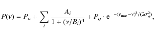
where Pn represents the white noise contribution and Ai and Bi are the amplitudes of the stellar background components and their characteristic frequencies (or inverse time scales), respectively. The frequency coverage which results from the 150 d CoRoT observations is sufficient to use three power law components. Pg,
We use a Bayesian Markov-Chain Monte Carlo (MCMC) algorithm to
fit the global model to the power density spectrum. The algorithm
samples a wide parameter space and delivers probability distributions
for all relevant quantities. The procedure is described in Gruberbauer et al. (2009)
and was originally designed to fit Lorentzian profiles to the p-mode
spectrum of a solar-type pulsator. Our problem is quite similar,
and it was trivial to adapt the code in order to fit a global
model to the power density spectra instead of a sequence of mode
profiles. The advantage of the algorithm is its stability and
insensitivity to wrong initial parameters, and also that it delivers
reliable parameters as well as realistic uncertainties in a fully
automatic way. For the frequency parameters (Bi)
we have sampled the entire frequency range of interest from 0
to 150 ![]() Hz.
For higher frequencies, the power spectra are potentially contaminated
by instrumental artifacts due to the satellites' orbital period. The
amplitude parameters (Pn, Ai,
and Pg)
were allowed to vary from zero to the highest amplitude peak in the
spectrum. Only
Hz.
For higher frequencies, the power spectra are potentially contaminated
by instrumental artifacts due to the satellites' orbital period. The
amplitude parameters (Pn, Ai,
and Pg)
were allowed to vary from zero to the highest amplitude peak in the
spectrum. Only
![]() and
and ![]() were kept within reasonable limits (0.5 to
2 times the value we inferred from a visual inspection of the
spectra). After some 500 000 iterations we calculated
the most probable value and its 1
were kept within reasonable limits (0.5 to
2 times the value we inferred from a visual inspection of the
spectra). After some 500 000 iterations we calculated
the most probable value and its 1![]() uncertainty for all
fitted parameters from their marginal distribution and constructed the
most probable global model fit.
uncertainty for all
fitted parameters from their marginal distribution and constructed the
most probable global model fit.
| Figure 1:
Marginal distributions of the Gaussian parameters (Eq. (2)) for the red
giant ``A'' as computed by the MCMC algorithm. Median
values and 1 |
|
| Open with DEXTER | |
![\begin{figure}
\par\includegraphics[width=8.5cm,clip]{11437fig2.eps}
\end{figure}](/articles/aa/full_html/2010/01/aa11437-08/img24.png)
|
Figure 2: Original (light-grey) and heavily smoothed (dark-grey) power density spectrum of the CoRoT exofield time series of the red giant A and a global model (black line) fitted to the power density spectrum. The model is a superposition of white noise (horizontal dashed line), three power law components (dashed lines) and a power excess hump approximated by a Gaussian function. The dotted line indicates the model fit plotted without the Gaussian component. |
| Open with DEXTER | |
![\begin{figure}
\par\includegraphics[width=17.5cm,clip]{11437fig3.eps}
\end{figure}](/articles/aa/full_html/2010/01/aa11437-08/img25.png)
|
Figure 3:
Fourier amplitude spectra for a sample of red giants observed by CoRoT.
Black lines indicate a global model fit, and dotted lines show the
model plotted without the Gaussian component and serve as a model for
the background signal. The center of the Gaussian is adopted to be the
frequency of maximum oscillation power,
|
| Open with DEXTER | |
As an example, we show in Fig. 1 the marginal distributions of the Gaussian parameters as computed by the MCMC algorithm for star A. The corresponding most probable global fit is given in Fig. 2 along with the original and heavily smoothed power density spectrum, the white noise, and power law components of the fit. Figure 3 shows a sequence of amplitude spectra selected from the 31 analyzed red giants with the corresponding global model fits. Note that the fits are calculated in power but are presented in amplitude for better visibility. The sequence impressively demonstrates that the frequency and amplitude range of the oscillations scale with the time scales and amplitudes of the background signal.
In a next step we use the white noise and power law components
of the global model (doted lines in Figs. 2 and 3) to correct
the power density spectra for the background signal, which should then
include only the oscillation signal. But what is more
interesting in this context, we assume the center of the Gaussian to
locate the centroid of the power excess hump, and as long as the power
excess hump is symmetric, the center of a Gaussian fit should equal the
frequency of maximum oscillation power. To test this
assumption we compute the weighted mean frequency, ![]() ,
in the frequency range of pulsations (
,
in the frequency range of pulsations (
![]()
![]()
![]() ), where we
use the residual power after correcting for the background signal as
weight. Although for seven of the eight stars shown in Fig. 3,
), where we
use the residual power after correcting for the background signal as
weight. Although for seven of the eight stars shown in Fig. 3, ![]() is
within
is
within ![]()
![]() 1
1![]() ,
,
![]() seems
to be systematically shifted towards higher frequencies. Indeed,
for 19 out of the 31 stars in our sample,
seems
to be systematically shifted towards higher frequencies. Indeed,
for 19 out of the 31 stars in our sample, ![]() is
higher than
is
higher than
![]() .
But as the average shift for the
19 stars (0.6%) is about four times smaller than the
stochastic error of
.
But as the average shift for the
19 stars (0.6%) is about four times smaller than the
stochastic error of
![]() ,
we expect the systematic error on our estimate of
,
we expect the systematic error on our estimate of
![]() to be negligible. Note that for the Sun the effect can not be
neglected. Based on SOHO/VIRGO data (Fröhlich
et al. 1997), we find
to be negligible. Note that for the Sun the effect can not be
neglected. Based on SOHO/VIRGO data (Fröhlich
et al. 1997), we find ![]() to be shifted by almost 2% towards higher frequencies.
to be shifted by almost 2% towards higher frequencies.
The second interesting parameter that can directly be
determined from the observed power spectrum is the large frequency
separation,
![]() ,
of consecutive radial overtone modes of the same spherical degree.
Since this frequency separation is, at least for the Sun (see,
e.g., Broomhall et al. 2009),
a function of the frequency itself, it is not
straightforward to identify an average value for all observed modes.
Such a value depends on the actual number and frequency range of the
observed modes and is difficult to compare for different observations.
We therefore specifically chose to define
,
of consecutive radial overtone modes of the same spherical degree.
Since this frequency separation is, at least for the Sun (see,
e.g., Broomhall et al. 2009),
a function of the frequency itself, it is not
straightforward to identify an average value for all observed modes.
Such a value depends on the actual number and frequency range of the
observed modes and is difficult to compare for different observations.
We therefore specifically chose to define
![]() as the average frequency separation in the frequency range of the
maximum oscillation power.
To identify
as the average frequency separation in the frequency range of the
maximum oscillation power.
To identify ![]() we use again the Bayesian MCMC algorithm (Gruberbauer
et al. 2009). But instead of fitting a
global model, we fit a sequence of equidistant Lorentzian profiles to
the power density spectra
we use again the Bayesian MCMC algorithm (Gruberbauer
et al. 2009). But instead of fitting a
global model, we fit a sequence of equidistant Lorentzian profiles to
the power density spectra
![\begin{displaymath}%
P(\nu) = P_n + \sum_{i=-2}^{2} \frac{a_{i}^2 \cdot \tau}{1 + 4[\nu - (\nu_0 +\Delta\nu \cdot i/2)]^2 \cdot (\pi \tau)^2},
\end{displaymath}](/articles/aa/full_html/2010/01/aa11437-08/img29.png)
where ai is the rms mode amplitude of the ith profile,
The advantage of our method compared to, e.g., the
comb-response function (Kjeldsen
et al. 1995) or an autocorrelation spectrum is that
it takes the Lorentzian-like form of the signal into account and is
therefore less sensitive to the stochastic nature of the signal.
Examples for the residual power density spectra and the most probable
fits are shown in Fig. 4.
Interestingly, the presence of additional modes which are not taken
into account in our model does not influence the fit. This can be seen
for instance from the power density spectrum of star A, where
the MCMC algorithm correctly identifies the l = 0
and 1 modes and does not consider the additional peaks at
about 72 and 79 ![]() Hz, which are most likely l = 2 modes.
We compare the marginal distributions for
Hz, which are most likely l = 2 modes.
We compare the marginal distributions for
![]() from our MCMC algorithm with the comb-response functions (both
with arbitrary ordinates) in the inserts of Fig. 3. Although for
some stars both methods give consistent results, the values can differ
by more that 0.2
from our MCMC algorithm with the comb-response functions (both
with arbitrary ordinates) in the inserts of Fig. 3. Although for
some stars both methods give consistent results, the values can differ
by more that 0.2 ![]() Hz.
Hz.
![\begin{figure}
\par\includegraphics[width=8.5cm,clip]{11437fig4.eps}
\end{figure}](/articles/aa/full_html/2010/01/aa11437-08/img32.png)
|
Figure 4:
Residual power density spectra for star A and B after
correcting for the background signal. The most probable model-fits used
to determine |
| Open with DEXTER | |
We expect this ambiguity to be due to the stochastic nature of the
signal. The observed time series represent a single realisation of a
damped and stochastically excited signal. Another realisation might
result in a different measurement for
![]() and
and
![]() .
In order to examine this we simulate different realisations of
the same solar-type oscillation signal. We use the original time series
of star A and pre-withen all significant peaks in the
frequency range of pulsation. The residual time series should now
include only the intrinsic background signal. We then generate
250 time series following the procedure in Chaplin
et al. (1997) with each data set representing a
different realisation of four radial orders of equidistant l = 0, 1,
and 2 modes with
.
In order to examine this we simulate different realisations of
the same solar-type oscillation signal. We use the original time series
of star A and pre-withen all significant peaks in the
frequency range of pulsation. The residual time series should now
include only the intrinsic background signal. We then generate
250 time series following the procedure in Chaplin
et al. (1997) with each data set representing a
different realisation of four radial orders of equidistant l = 0, 1,
and 2 modes with ![]() =
7.20
=
7.20 ![]() Hz
and an arbitrary value for
Hz
and an arbitrary value for ![]() =
=
![]() =
1
=
1 ![]() Hz.
The time domain rms amplitudes of radial and l =
1 modes are set in a way that the mode heights follow the
Gaussian shape of the original power excess hump. The rms amplitudes of
l = 2 modes are set arbitrarily to
half the value of the closest radial mode. The largest amplitude mode
is centered on 76.2
Hz.
The time domain rms amplitudes of radial and l =
1 modes are set in a way that the mode heights follow the
Gaussian shape of the original power excess hump. The rms amplitudes of
l = 2 modes are set arbitrarily to
half the value of the closest radial mode. The largest amplitude mode
is centered on 76.2 ![]() Hz,
and all modes have a lifetime of 20 days, which is a typical
value for intermediate luminous red giants (Dupret
et al. 2009) and corresponds to what we have found
for the intrinsic modes. Finally we superpose each simulated data set
with the residual time series, calculate the power density spectrum,
and apply our algorithms to determine
Hz,
and all modes have a lifetime of 20 days, which is a typical
value for intermediate luminous red giants (Dupret
et al. 2009) and corresponds to what we have found
for the intrinsic modes. Finally we superpose each simulated data set
with the residual time series, calculate the power density spectrum,
and apply our algorithms to determine
![]() and
and
![]() .
The simulations give an average value
.
The simulations give an average value
![]() =
74.42
=
74.42 ![]() Hz
with a rms scatter of 0.55
Hz
with a rms scatter of 0.55 ![]() Hz, which is
well within the 1
Hz, which is
well within the 1![]() uncertainty
of the originally determined value (74.32
uncertainty
of the originally determined value (74.32 ![]() 0.81
0.81 ![]() Hz). The
situation is different for
Hz). The
situation is different for
![]() .
If we determine
.
If we determine ![]() from the frequency of the largest peak of the comb-response function,
then the stochastic nature of the signal adds a rms scatter of about
0.21
from the frequency of the largest peak of the comb-response function,
then the stochastic nature of the signal adds a rms scatter of about
0.21 ![]() Hz
in our simulation. This is much compared to the
rms scatter of only 0.04
Hz
in our simulation. This is much compared to the
rms scatter of only 0.04 ![]() Hz if we use our Bayesian MCMC approach,
which is again compatible with the 1
Hz if we use our Bayesian MCMC approach,
which is again compatible with the 1![]() uncertainty of the
original value (0.04
uncertainty of the
original value (0.04 ![]() Hz). This assures us that the stochastic nature
of the oscillation signal adds no significant additional uncertainty in
our subsequent analysis. We list
Hz). This assures us that the stochastic nature
of the oscillation signal adds no significant additional uncertainty in
our subsequent analysis. We list
![]() ,
,
![]() and the corresponding 1
and the corresponding 1![]() uncertainties
for our sample of red giants in Table 2.
uncertainties
for our sample of red giants in Table 2.
4 Asteroseismic determination of fundamental parameters
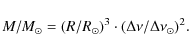
Stellar masses of field stars are usually determined by comparing the location in the H-R diagram with evolutionary tracks. But when stars evolve to become red giants, their evolutionary tracks move together and a relatively narrow range in the H-R diagram covers a large range in mass. Consequently, the mass determined from a location in the H-R diagram becomes quite uncertain. Additionally, the actual position and slope of the red-giant branch in stellar evolutionary calculations depend very much on the parameters used to compute the models. It is, however, believed that the global properties of solar-type oscillations, like the frequency range where they can be observed, depend on the fundamental parameters of the star. It should therefore be possible to determine these parameters from global properties of the observed oscillations.
The amplitudes of solar oscillations are modulated by a broad
envelope with its maximum at a frequency of about 3 mHz. The
center and the shape of the envelope is defined by the excitation and
damping where the later can be assumed to be Gaussian
(see previous section). Brown
et al. (1991) and latter on Kjeldsen
& Bedding (1995) have shown that the frequency of
maximum oscillation power, ![]() ,
of p-mode oscillations scales to good approximation with the acoustic
cutoff frequency, which sets limits on the maximum frequency for
acoustic oscillations. They predict
,
of p-mode oscillations scales to good approximation with the acoustic
cutoff frequency, which sets limits on the maximum frequency for
acoustic oscillations. They predict
![]() by scaling from the Sun as
by scaling from the Sun as
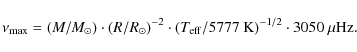
It has been shown that this simple scaling relation gives very good estimates for the frequency of maximum oscillation power for less evolved stars (e.g. Bedding & Kjeldsen 2003), but it cannot a priori be assumed that it holds also for stars of the giant branch. Stello et al. (2008), however, have demonstrated for a number of bright red giants observed by the star tracker of the WIRE satellite that the measured
Table 1: Mass and radius of stars used to test our asteroseismic mass and radius determination approach.
Our sample of red giants is far too faint to measure
parallaxes. But the CoRoT observations are significantly
better than the WIRE observations in terms of duration and
precision, which enables us to also extract the large frequency
separation. For the Sun, Toutain
& Fröhlich (1992) have determined a large frequency
separation of about 134.92 ![]() Hz at the radial order where the maximum
oscillation power is seen (n = 21).
The large frequency separation reflects essentially the global
properties of the star and is believed to scale with the dynamical time
scale and therefore with the square root of the mean density. Kjeldsen & Bedding (1995)
predicted
Hz at the radial order where the maximum
oscillation power is seen (n = 21).
The large frequency separation reflects essentially the global
properties of the star and is believed to scale with the dynamical time
scale and therefore with the square root of the mean density. Kjeldsen & Bedding (1995)
predicted ![]() by scaling from the Sun as
by scaling from the Sun as
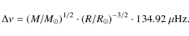
Knowing
We have tested this method for a number of well-known solar-type pulsators and compare in Table 1 the seismic masses and radii with independent measurements given in the literature (last two columns). The specific values for the latter are taken from
- Arcturus:
 and
and  are given by Tarrant et al.
(2007) and Retter
et al. (2003), respectively. The radius is based on
the Hipparcos parallax (van Leeuwen 2007)
and interferometric measurements (Lacour
et al. 2008). The mass range is estimated from the
average surface gravity listed in the VizieR
database (
are given by Tarrant et al.
(2007) and Retter
et al. (2003), respectively. The radius is based on
the Hipparcos parallax (van Leeuwen 2007)
and interferometric measurements (Lacour
et al. 2008). The mass range is estimated from the
average surface gravity listed in the VizieR
database (
 = 1.72
  0.2)
and the interferometric radius.
0.2)
and the interferometric radius.
- HD 181907: we determine
from the CoRoT observations published in Carrier
et al. (2009), who also derived
.
The mass is estimated from a comparison between the star's position in
the H-R diagram and metal-poor evolutionary tracks.
 Oph:
and
were determined from unpublished MOST photometry. The radius
is based on the Hipparcos parallax (van
Leeuwen 2007) and interferometric measurements (Richichi et al. 2005). An
upper limit for the mass is estimated from the average surface gravity
(
= 2.42 0.3)
taken from the VizieR database and the interferometric radius.
Oph:
and
were determined from unpublished MOST photometry. The radius
is based on the Hipparcos parallax (van
Leeuwen 2007) and interferometric measurements (Richichi et al. 2005). An
upper limit for the mass is estimated from the average surface gravity
(
= 2.42 0.3)
taken from the VizieR database and the interferometric radius.
 Oph:
and
are given by Kallinger et al.
(2008), who determined the mass from a detailed comparison of
observed and model frequencies. The radius is based on the Hipparcos
parallax (van Leeuwen 2007) and
interferometric measurements (Richichi
et al. 2005).
Oph:
and
are given by Kallinger et al.
(2008), who determined the mass from a detailed comparison of
observed and model frequencies. The radius is based on the Hipparcos
parallax (van Leeuwen 2007) and
interferometric measurements (Richichi
et al. 2005).
 Hya:
,
,
and the mass are taken from Frandsen
et al. (2002), where they estimate the mass from a
comparison between the star's position in the H-R diagram and
solar-calibrated evolutionary tracks. We derive
from a weighted average of the published frequencies.
Hya:
,
,
and the mass are taken from Frandsen
et al. (2002), where they estimate the mass from a
comparison between the star's position in the H-R diagram and
solar-calibrated evolutionary tracks. We derive
from a weighted average of the published frequencies.
- M 67 13:
and
are determined from the photometric time series kindly provided by
Stello. The mass is estimated from isochrone fits to the
color-magnitude diagram of M 67 (Stello
et al. 2007).
 Ind:
is given by Carrier et al.
(2007).
is taken from Bedding et al.
(2006), who also provide a mass range based on a comparison
between the star's position in the H-R diagram and
evolutionary tracks.
Ind:
is given by Carrier et al.
(2007).
is taken from Bedding et al.
(2006), who also provide a mass range based on a comparison
between the star's position in the H-R diagram and
evolutionary tracks.
 Her
A: ,
,
and the mass are taken from Martic
et al. (2001).
Her
A: ,
,
and the mass are taken from Martic
et al. (2001).
- Hyi:
and
are given by Kjeldsen et al.
(2005) and Bedding
et al. (2001), respectively. The radius is based on
interferometric measurements from North
et al. (2007), who also provide a summary of
non-seismically determined values for the mass.
- HD 49933:
and
are given by Kallinger et al.
(2009), who determined the mass from a detailed comparison of
observed and model frequencies.
 Ara:
and
were extracted from Bouchy
et al. (2005). A non-seismic estimate for
the mass can be found in Bazot
et al. (2005).
Ara:
and
were extracted from Bouchy
et al. (2005). A non-seismic estimate for
the mass can be found in Bazot
et al. (2005).
 Cen
A & B:
and
are taken from Kjeldsen et al.
(2005). Masses were determined by Guenther
& Demarque (2000) using Hipparcos parallaxes and the
binary mass ratio.
Cen
A & B:
and
are taken from Kjeldsen et al.
(2005). Masses were determined by Guenther
& Demarque (2000) using Hipparcos parallaxes and the
binary mass ratio.
Table 2: Summary for the analysed sample of red gaints.
![\begin{figure}
\par\includegraphics[width=16.5cm,clip]{11437fig5.eps}
\end{figure}](/articles/aa/full_html/2010/01/aa11437-08/img50.png)
|
Figure 5:
Theoretical H-R diagram showing the location of the stars used to test
our asteroseismic mass and radius determination approach. Grey-filled
dots (total sample) and black dots (stars presented in Fig. 3) indicate the
analyzed CoRoT pulsating red giants where the actual position in the
HR-diagram is based on a comparison with evolutionary tracks. The
errors bars correspond to the approximate uncertainties of our method
and are significantly larger than the observationally based errors.
Dashed black lines indicate isopleths for
|
| Open with DEXTER | |
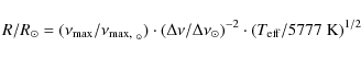
If not explicitly mentioned the radius is determined according to
![]() with the effective temperature and luminosity taken from the listed
reference (or references therein). Although
with the effective temperature and luminosity taken from the listed
reference (or references therein). Although
![]() is in some cases only a rough estimate from a published power spectrum,
our approach yields quite accurate masses and radii in a large portion
of the H-R diagram. For faint stars it often turns
out that no or only poor estimates for the effective temperature are
available. This is, however, not very critical for stars on
the giant branch, as
is in some cases only a rough estimate from a published power spectrum,
our approach yields quite accurate masses and radii in a large portion
of the H-R diagram. For faint stars it often turns
out that no or only poor estimates for the effective temperature are
available. This is, however, not very critical for stars on
the giant branch, as
![]() depends only on the square
root of
depends only on the square
root of
![]() ,
and pulsating red giants are expected to populate only a
relatively narrow temperature range (
,
and pulsating red giants are expected to populate only a
relatively narrow temperature range (![]() 4200 to 5300 K). It should
therefore be possible to get a reasonable asteroseismic mass and radius
for red giants even if an accurate
4200 to 5300 K). It should
therefore be possible to get a reasonable asteroseismic mass and radius
for red giants even if an accurate
![]() is not available. This is
shown for the red giants in Table 1 (Arcturus to
is not available. This is
shown for the red giants in Table 1 (Arcturus to ![]() Hya),
where we ignore the known values for
Hya),
where we ignore the known values for
![]() and fix the temperature to a
typical value of 4750 K.
and fix the temperature to a
typical value of 4750 K.
For our CoRoT sample of red giants we first estimate the effective temperature from 2MASS photometric colors and color-temperature calibrations (Masana et al. 2006; González Hernández & Bonifacio 2009). Unfortunately, both calibrations result in temperatures which are systematically too cool. The average temperature resulting from the Masana et al. (2006) calibration is about 3820 K, which would make our sample of red giants either extremely metal rich or would put all the stars high up on the giant branch. Both explanations are not very plausible. We expect the discrepancy to be due to severe reddening which is difficult to estimate for such faint (and therefore distant) stars. The situation is sligthly better for the González Hernández & Bonifacio (2009) calibration, but we decided to ignore the effective temperatures determined from color-temperature calibrations.
Instead, we use a different approach. We calculate an initial
guess for the mass and radius from Eqs. (5) and (6) by fixing the
effective temperature to a typical value of 4750 K.
In a next step we compare the initial mass and radius
to those of a grid of solar-calibrated red giant models. Interpolation
in the grid gives a better estimate for the temperature, which is used
as a new input for Eq. (5).
After about three iterations the procedure converges to a certain
location in the H-R diagram where the final locus in the
H-R diagram is independent from the starting value
for
![]() as long as the initial value
is kept within the temperature range of
our model grid (
as long as the initial value
is kept within the temperature range of
our model grid (![]() 4000-5500 K).
4000-5500 K).
The resulting fundamental parameters and their uncertainties
are given in Table 2.
The errors are based only on the uncertainties for
![]() and
and ![]() and range from 1.5 to 8.2% and 3.9
to 17% for the radius and mass, respectively. V magnitudes
listed in Table 2
are taken from the EXODAT database (Deleuil et al. 2006).
and range from 1.5 to 8.2% and 3.9
to 17% for the radius and mass, respectively. V magnitudes
listed in Table 2
are taken from the EXODAT database (Deleuil et al. 2006).
The red-giant models used to estimate the effective
temperatures fall along evolutionary tracks computed with the Yale
Stellar Evolution Code YREC (Demarque et al. 2007; Guenther
et al. 1992). The evolutionary tracks were computed
for an initial helium and metal mass fraction (Y, Z) =
(0.28, 0.02) with the mixing-length parameter ![]() = 1.8
set to approximately meet the Sun's position in the
H-R diagram with a one-solar-mass model at roughly the solar
age. Note, although the models are not exactly calibrated to the Sun,
we refer to them as solar-calibrated in the
following. A more detailed description of the used model
physics can be found in Kallinger
et al. (2008) or Kallinger
(2009) and references therein.
= 1.8
set to approximately meet the Sun's position in the
H-R diagram with a one-solar-mass model at roughly the solar
age. Note, although the models are not exactly calibrated to the Sun,
we refer to them as solar-calibrated in the
following. A more detailed description of the used model
physics can be found in Kallinger
et al. (2008) or Kallinger
(2009) and references therein.
In Fig. 5
we show our sample of red giants in the H-R diagram along with
the test stars (Table 1)
and contours of constant
![]() and
and
![]() .
We whish to emphasize that the actual locations of the red giants are
specific to the model grid used to estimate their effective
temperatures. We assume that all red giants are comparable to the Sun
in terms of their initial chemical composition and mixing-length
parameter. This might be correct for some of them but not for others.
The effective temperature and luminosity of a model with a given mass
and radius do not only depend on the model's age but also for instance
on the initial chemical composition of the model. Metal-poor models,
e.g., are shifted towards higher surface temperatures and luminosities
compared to solar-abundant models. On the other hand, low and
intermediate mass red giants contract rapidly after they have reached
the tip of the red giant branch (RGB) to settle on the He-core burning
main sequence at a somewhat higher temperature before they start to
climb the asymptotic giant branch (ABG). In other
words, a red giant with a given mass and radius is located at different
positions in the H-R diagram depending on, e.g., the
chemical composition and/or the evolutionary stage.
.
We whish to emphasize that the actual locations of the red giants are
specific to the model grid used to estimate their effective
temperatures. We assume that all red giants are comparable to the Sun
in terms of their initial chemical composition and mixing-length
parameter. This might be correct for some of them but not for others.
The effective temperature and luminosity of a model with a given mass
and radius do not only depend on the model's age but also for instance
on the initial chemical composition of the model. Metal-poor models,
e.g., are shifted towards higher surface temperatures and luminosities
compared to solar-abundant models. On the other hand, low and
intermediate mass red giants contract rapidly after they have reached
the tip of the red giant branch (RGB) to settle on the He-core burning
main sequence at a somewhat higher temperature before they start to
climb the asymptotic giant branch (ABG). In other
words, a red giant with a given mass and radius is located at different
positions in the H-R diagram depending on, e.g., the
chemical composition and/or the evolutionary stage.
To illustrate this ambiguity we compare stellar models for a
given mass and radius, but with different initial chemical composition
and during different evolutionary stages. The result is shown in
Fig. 6
where we illustrate that 2.5 ![]() RGB models with 10
RGB models with 10 ![]() with a initial chemical composition of (Y, Z) =
(0.25, 0.01) and (0.32, 0.04) are about
155 K hotter and 13% more luminous and about
135 K cooler and 11% less luminous, respectively,
than a solar-calibrated RGB model with the same mass
and radius. Similar results can be expected for different mixing-length
parameters. Whereas the parameterization of convection has only small
effects on the surface properties of a star during early evolution,
different mixing-length parameters result in quite different
evolutionary tracks when the star ascends the giant branch. This is
because the mixing-length parameter sets the temperature gradient in
the convective regions and thus controls how efficiently energy can be
deduced from the interior. Consequently, the mixing-length parameter
defines at what stage the star starts to climb the giant branch during
the hydrogen shell burning phase. A slightly smaller effect
can be expected for the different evolutionary stages.
Our 2.5
with a initial chemical composition of (Y, Z) =
(0.25, 0.01) and (0.32, 0.04) are about
155 K hotter and 13% more luminous and about
135 K cooler and 11% less luminous, respectively,
than a solar-calibrated RGB model with the same mass
and radius. Similar results can be expected for different mixing-length
parameters. Whereas the parameterization of convection has only small
effects on the surface properties of a star during early evolution,
different mixing-length parameters result in quite different
evolutionary tracks when the star ascends the giant branch. This is
because the mixing-length parameter sets the temperature gradient in
the convective regions and thus controls how efficiently energy can be
deduced from the interior. Consequently, the mixing-length parameter
defines at what stage the star starts to climb the giant branch during
the hydrogen shell burning phase. A slightly smaller effect
can be expected for the different evolutionary stages.
Our 2.5 ![]() and 10
and 10 ![]() is about 60 K hotter and 5% more luminous in its
AGB phase than the corresponding RGB model. Although
most of our sample red giants are expected to have a mass below
2.5
is about 60 K hotter and 5% more luminous in its
AGB phase than the corresponding RGB model. Although
most of our sample red giants are expected to have a mass below
2.5 ![]() ,
we use here the more massive models. This is because YREC,
just like other stellar evolution codes, is not able to follow the
explosive He flash in low mass stars, and we currently have no
AGB starting models available. We can follow the
He core ignition only for higher mass models and evolve models
on the AGB. We do not expect the effect to be significantly
different for lower mass models, however.
,
we use here the more massive models. This is because YREC,
just like other stellar evolution codes, is not able to follow the
explosive He flash in low mass stars, and we currently have no
AGB starting models available. We can follow the
He core ignition only for higher mass models and evolve models
on the AGB. We do not expect the effect to be significantly
different for lower mass models, however.
We have demonstrated in Fig. 6 that an
unknown chemical composition, mixing-length parameter, and evolutionary
stage adds a certain amount of uncertainty when we determine a star's
position in the H-R diagram from its mass and radius. This
ambiguity will add additional uncertainties on the asteroseismic masses
and radii. To quantify this effect we have computed additional
sets of evolutionary tracks. For the sake of simplicity and as we
expect the uncertainty to be smaller for an unknown evolutionary stage
than for an unknown initial chemical composition we concentrate here on
models with different initial chemical compositions, namely (Y,
Z) = (0.25, 0.01) and
(0.32, 0.04). In Table 3 we compare the
fundamental parameters as they result from using the different model
grids to estimate the effective temperature for Eq. (5). We list here only
three stars (A, E, and H from Table 2) which are,
however, selected to cover the range of interest in the
H-R diagram. The spread in chemical composition adds an
additional uncertainty of not more than about 1.8
and 5.5% on the radius and mass, respectively,
which is smaller or at most comparable to the observationally
based errors. The situation is different for the effective temperature
and luminosity where the additional uncertainties are significantly
larger than the observational errors. To account for this we
have extended the error bars in Fig. 5 to ![]() 150 K
and
150 K
and ![]() 17%
for the effective temperature and luminosity, respectively. Note that
these are still quite accurate fundamental parameters for such faint
stars.
17%
for the effective temperature and luminosity, respectively. Note that
these are still quite accurate fundamental parameters for such faint
stars.
![\begin{figure}
\par\includegraphics[width=8.8cm,clip]{11437fig6.eps}
\end{figure}](/articles/aa/full_html/2010/01/aa11437-08/img52.png)
|
Figure 6:
YREC evolutionary tracks for 2.5 |
| Open with DEXTER | |
From Eqs. (3)
and (4)
and the isopleths for ![]() and
and ![]() in Fig. 5
it is obvious that the two parameters are correlated to some extent.
Both parameters depend on the stellar mass and radius. Stello et al. (2009) indeed
found a tight relation between
in Fig. 5
it is obvious that the two parameters are correlated to some extent.
Both parameters depend on the stellar mass and radius. Stello et al. (2009) indeed
found a tight relation between
![]() and
and ![]() for main-sequence and red-giant stars, which was confirmed by Hekker et al. (2009) for
CoRoT red giants. Although the relation seems to be very tight,
no exact relation can be explained from a
theoretical point of view. It even turns out that the relation
between
for main-sequence and red-giant stars, which was confirmed by Hekker et al. (2009) for
CoRoT red giants. Although the relation seems to be very tight,
no exact relation can be explained from a
theoretical point of view. It even turns out that the relation
between ![]() and
and ![]() strongly depends on the stellar mass. This can be seen from
Fig. 7,
where we compare the ratio between
strongly depends on the stellar mass. This can be seen from
Fig. 7,
where we compare the ratio between
![]() and
and ![]() as a function of
as a function of ![]() for models of different evolutionary tracks with the sample of red
giants. The ordinate basically represents the inverse radial order
where the maximum oscillation power is seen (Kjeldsen
& Bedding 1995). We introduce this diagram as a sort
of diagnostic asteroseismic diagram similar to a diagram which is
usually used to estimate the mass and central hydrogen abundance for
solar-type pulsators close to or on the main sequence from the measured
large and small frequency separations (see e.g., Roxburgh
& Vorontsov 2003). Our diagnostic asteroseismic
diagram is particularly useful on the giant branch and relies on an
observational quantity, namely
for models of different evolutionary tracks with the sample of red
giants. The ordinate basically represents the inverse radial order
where the maximum oscillation power is seen (Kjeldsen
& Bedding 1995). We introduce this diagram as a sort
of diagnostic asteroseismic diagram similar to a diagram which is
usually used to estimate the mass and central hydrogen abundance for
solar-type pulsators close to or on the main sequence from the measured
large and small frequency separations (see e.g., Roxburgh
& Vorontsov 2003). Our diagnostic asteroseismic
diagram is particularly useful on the giant branch and relies on an
observational quantity, namely
![]() ,
which is easier to determine than the small frequency separation. Other
parameters like the helium core abundance can easily be added to this
diagram. The diagram also demonstrates the relative robustness of our
method to determine an asteroseismic mass and radius. Models of a given
mass and radius (large dots) are only slightly shifted in the diagram
if e.g. their initial chemical composition is significantly
changed.
,
which is easier to determine than the small frequency separation. Other
parameters like the helium core abundance can easily be added to this
diagram. The diagram also demonstrates the relative robustness of our
method to determine an asteroseismic mass and radius. Models of a given
mass and radius (large dots) are only slightly shifted in the diagram
if e.g. their initial chemical composition is significantly
changed.
We have illustrated to some extent what uncertainty can be
expected for a red giant's position in the H-R diagram if the
star's initial chemical composition and/or mixing-length parameter
and/or evolutionary stage is unknown. But there are also other effects
in stellar evolution which carry a similar type of uncertainty.
Examples are the overshoot parameter or a better description of
convection than the MLT which change the
![]() relations.
These effects are difficult to estimate and are not on the scope of the
current analysis.
relations.
These effects are difficult to estimate and are not on the scope of the
current analysis.
Table 3: Fundamental parameters as they follow from a metal-poor (MP), solar-calibrated (SC), or metal rich (MR) grid.
![\begin{figure}
\par\includegraphics[width=8.8cm,clip]{11437fig7.eps}
\end{figure}](/articles/aa/full_html/2010/01/aa11437-08/img55.png)
|
Figure 7:
Diagnostic asteroseismic diagram for stars on the red-giant branch.
Solid lines correspond to solar-calibrated evolutionary tracks. The
dotted lines indicate models with 1.5 |
| Open with DEXTER | |
5 Conclusions and prospects
We have shown that global properties of solar-type pulsations can be used to derive estimates for the stellar mass and radius by employing well-established and often used scaling relations. We have tested this approach on various prominent solar-type pulsators and applied it to a first sample of red giant pulsators observed by CoRoT. Despite the mentioned approximations the derived fundamental parameters can serve to constrain the starting values for a more detailed analysis.
We note that we do not stop at this point. In a next step we will use the integral of the Gaussian part of our global power density model to deduce the total spectral power of solar-type pulsations, which we expect to scale with the luminosity-mass ratio. This, however, needs extensive calibration for solar-type pulsators with independently determined fundamental parameters, which we are currently carrying out. We believe that we can, for the first time, derive all basic fundamental parameters (mass, radius, luminosity, and consequently also the effective temperature) of a solar-type pulsator by simply measuring global properties of its oscillations in the power density spectrum. This will have influence on various astrophysical applications. One can use it as a distance indicator, or one can study the behavior of convective time scales of stars as a function of their position in the H-R diagram. By comparing the individual pulsation frequencies with theoretical eigenfrequencies it should be possible to investigate the parameterization of convective models (e.g., the mixing-length parameter) in a region of the H-R diagram where stars are very sensitive to these parameters.
Finally, we want to mention that we will apply our asteroseismic fundamental parameter determination to all pulsating red giants observed by CoRoT, and also we plan to arrange an online database for them.
AcknowledgementsT.K., M.G., and W.W.W. are supported by the Austrian Research Promotion Agency (FFG), and the Austrian Science Fund (FWF P17580). T.K. is also supported by the Canadian Space Agency. The research leading to these results has received funding from the Research Council of K.U. Leuven under grant agreement GOA/2008/04 and from the Belgian PRODEX Office under contract C90309: CoRoT Data Exploitation. F.C. is a postdoctoral fellow of the Fund for Scientific Research, Flanders. A.P.H. acknowledges the support grant 50OW0204 from the Deutsches Zentrum für Luft- und Raumfahrt e. V. (DLR). S.H. acknowledges financial support from the Belgian Federal Science Policy (Ref.: MO/33/018). C.C. is supported partially be a CITA national fellowship. Furthermore, it is a pleasure to thank D. Stello (University of Sydney) for providing us with the photometric data of M 67. We thank the MOST Science Team for letting us use the unpublished photometry of
References
- Aigrain, S., Favata, F., & Gilmore, G. 2004, A&A, 414, 1139 [Google Scholar]
- Baglin, A. 2006, The CoRoT mission, pre-launch status, stellar seismology and planet nding, ed. M. Fridlund, A. Baglin, J. Lochard, & L. Conroy, ESA Publication Division, Noordwijk, The Netherlands, ESA SP-1306 [Google Scholar]
- Barban, C., Matthews, J. M., De Ridder, J., et al. 2007, A&A, 468, 1033 [Google Scholar]
- Bazot, M., Vauclair, S., Bouchy, F., & Santos, N. C. 2005, A&A, 440, 615 [Google Scholar]
- Bedding, T. R., & Kjeldsen, H. 2003, PASA, 20, 203 [Google Scholar]
- Bedding, T. R., Butler, R. P., Kjeldsen, H., et al. 2001, ApJ, 549, L105 [NASA ADS] [CrossRef] [Google Scholar]
- Bedding, T. R., Butler, R. P., Fabien, C., et al. 2006, ApJ, 647, 558 [NASA ADS] [CrossRef] [Google Scholar]
- Bouchy, F., Bazot, M., Santos, N. C., et al. 2005, A&A, 440, 609 [Google Scholar]
- Broomhall, A.-M., Chaplin, W. J., Davies, G. R., et al. 2009, MNRAS, 396, L100 [NASA ADS] [CrossRef] [Google Scholar]
- Brown, T. M., Gilliland, R. L., Noyes, R. W., & Ramsey, L. W. 1991, ApJ, 368, 599 [NASA ADS] [CrossRef] [Google Scholar]
- Carrier, F., Kjeldsen, H., Bedding, T. R., et al. 2007, A&A, 470, 1059 [Google Scholar]
- Carrier, F., De Ridder, J., Baudin, F., et al. 2009, A&A, in press [Google Scholar]
- Cox, J. P. 1980, Theory of stellar pulsation (Princeton University Press) [Google Scholar]
- Chaplin, W. J., Elsworth, Y., Howe, R., et al. 1997, MNRAS, 287, 51 [NASA ADS] [CrossRef] [Google Scholar]
- Deleuil, M., Moutou, C., Deeg, H. J., et al. 2006, The CoRoT mission, pre-launch status, stellar seismology and planet nding, ed. M. Fridlund, A. Baglin, J. Lochard, & L. Conroy, ESA Publication Division, Noordwijk, The Netherlands, ESA SP-1306 [Google Scholar]
- Demarque, P., Guenther, D. B., Li, L. H., Mazumdar, A., & Straka, C. W. 2007, Ap&SS, 447 [arXiv:0710.4003] [Google Scholar]
- De Ridder, J., Barban, C., Baudin, F., et al. 2009, Nature, 459, 398 [Google Scholar]
- Dupret, M.-A., Belkacem, K., Samadi, R., et al. 2009, A&A, 506, 57 [Google Scholar]
- Eggenberger, P., Charbonnel, C., Talon, S., et al. 2004, A&A, 417, 235 [Google Scholar]
- Frandsen, S., Carrier, F., Aerts, C., et al. 2002, A&A, 394, L5 [Google Scholar]
- Fröhlich, C., Andersen, B. N., Appourchaux, T., et al. 1997, Sol. Phys., 170, 1 [NASA ADS] [CrossRef] [Google Scholar]
- Gilliland, R. 2008, ApJ, 136, 566 [Google Scholar]
- Gonález Hernández, J. I., & Bonifacio, P. 2009, A&A, 497, 497 [Google Scholar]
- Gruberbauer, M., Kallinger, T., & Weiss, W. W. 2009, A&A, 506, 1043 [Google Scholar]
- Guenther, D. B., & Demarque, P. 2000, ApJ, 531, 503 [NASA ADS] [CrossRef] [Google Scholar]
- Guenther, D. B., Demarque, P., Kim, Y.-C., & Pinsonneault, M. H. 1992, ApJ, 387, 372 [NASA ADS] [CrossRef] [Google Scholar]
- Harvey, J. 1985, in Future Missions in Solar, Heliospheric & Space Plasma Physics, ed. E. Rolfe, & B. Battrick, ESA SP, 235, 199 [Google Scholar]
- Hekker, S., Aerts, C., De Ridder, J., & Carrier, F. 2006, A&A, 458, 931 [Google Scholar]
- Hekker, S., Kallinger, T., Baudin, F., et al. 2009, A&A, 506, 465 [Google Scholar]
- Houdek, G., & Gough, D. O. 2002, MNRAS, 336, L65 [NASA ADS] [CrossRef] [Google Scholar]
- Kallinger, T. 2009, Ph.D. Thesis, University of Vienna, Austria [Google Scholar]
- Kallinger, T., Guenther, D. B., Matthews, J. M., et al. 2008, A&A, 478, 497 [Google Scholar]
- Kallinger, T., Gruberbauer, M., Guenther, D. B., et al. 2009, A&A, accepted [arXiv:0811.4686v1] [Google Scholar]
- Kjeldsen, H., & Bedding, T. R. 1995, A&A, 293, 87 [Google Scholar]
- Kjeldsen, H., Bedding, T. R., Viskum, M., & Frandsen, S. 1995, ApJ, 109, 1313 [Google Scholar]
- Kjeldsen, H., Bedding, T. R., Butler, R. P., et al. 2005, ApJ, 635, 1281 [NASA ADS] [CrossRef] [Google Scholar]
- Lacour, S., Meimon, S., Thiebaut, E., et al. 2009, A&A, 485, 561 [Google Scholar]
- Martic, M., Lebrun, J. C., Schmitt, J., et al. 2001, ESASP, 464, 431 [Google Scholar]
- Masana, E., Jordi, C., & Ribas, I. 2006, A&A, 450, 735 [Google Scholar]
- Michel, E., Samadi, R., Baudin, F., et al. 2009, A&A, 495, 979 [Google Scholar]
- North, J. R., Davis, J., Bedding, T. R., et al. 2007, MNRAS, 380, L80 [NASA ADS] [CrossRef] [Google Scholar]
- Retter, A., Bedding, T. R., Buzasi, D. L., et al. 2003, ApJ, 591, L151 [NASA ADS] [CrossRef] [Google Scholar]
- Richichi, A., Percheron, I., & Khristoforova, M. 2005, A&A, 431, 773 [Google Scholar]
- Roxburgh, I. W., & Vorontsov, S. V. 2003, A&A, 411, 220 [Google Scholar]
- Samadi, R., Fialho, F., Costa, J. E. S., et al. 2006, The CoRoT mission, pre-launch status, stellar seismology and planet nding, ed. M. Fridlund, A. Baglin, J. Lochard, & L. Conroy, ESA Publication Division, Noordwijk, The Netherlands, ESA SP-1306 [arXiv:0703.354v1] [Google Scholar]
- Stello, D., Kjeldsen, H., Bedding, T. R., & Buzasi, D. 2006, A&A, 448, 709 [Google Scholar]
- Stello, D., Bruntt, H., Kjeldsen, H., et al. 2007, MNRAS, 377, 584 [NASA ADS] [CrossRef] [Google Scholar]
- Stello, D., Bruntt, H., Preston, H., & Buzasi, D. 2008, ApJ, 674, L53 [NASA ADS] [CrossRef] [Google Scholar]
- Stello, D., Chaplin, W. J., Basu, S., Elsworth, Y. P., & Bedding, T. R. 2009, MNRAS, 400, L80 [NASA ADS] [CrossRef] [Google Scholar]
- Tarrant, N. J., Chaplin, W. J., Elsworth, Y., et al. 2007, MNRAS, 382, L48 [NASA ADS] [CrossRef] [Google Scholar]
- Tassoul, M. 1980, ApJS, 43, 469 [NASA ADS] [CrossRef] [Google Scholar]
- Toutain, T., & Fröhlich, C. 1992, A&A, 257, 287 [Google Scholar]
- van Leeuwen, F. 2007, A&A, 474, 653 [Google Scholar]
Footnotes
- ... determination
- The CoRoT (Convection, Rotation, and planetary Transits) space mission, launched on 2006 December 27, was developed and is operated by the CNES, with participation of the Science Programs of ESA, ESAs RSSD, Austria, Belgium, Brazil, Germany and Spain.
- ... page
- http://idoc-corot.ias.u-psud.fr/
- ... VizieR
- http://vizier.u-strasbg.fr/viz-bin/VizieR
All Tables
Table 1: Mass and radius of stars used to test our asteroseismic mass and radius determination approach.
Table 2: Summary for the analysed sample of red gaints.
Table 3: Fundamental parameters as they follow from a metal-poor (MP), solar-calibrated (SC), or metal rich (MR) grid.
All Figures
| |
Figure 1:
Marginal distributions of the Gaussian parameters (Eq. (2)) for the red
giant ``A'' as computed by the MCMC algorithm. Median
values and 1 |
| Open with DEXTER | |
| In the text | |
|
|
Figure 2: Original (light-grey) and heavily smoothed (dark-grey) power density spectrum of the CoRoT exofield time series of the red giant A and a global model (black line) fitted to the power density spectrum. The model is a superposition of white noise (horizontal dashed line), three power law components (dashed lines) and a power excess hump approximated by a Gaussian function. The dotted line indicates the model fit plotted without the Gaussian component. |
| Open with DEXTER | |
| In the text | |
|
|
Figure 3:
Fourier amplitude spectra for a sample of red giants observed by CoRoT.
Black lines indicate a global model fit, and dotted lines show the
model plotted without the Gaussian component and serve as a model for
the background signal. The center of the Gaussian is adopted to be the
frequency of maximum oscillation power,
|
| Open with DEXTER | |
| In the text | |
|
|
Figure 4:
Residual power density spectra for star A and B after
correcting for the background signal. The most probable model-fits used
to determine |
| Open with DEXTER | |
| In the text | |
|
|
Figure 5:
Theoretical H-R diagram showing the location of the stars used to test
our asteroseismic mass and radius determination approach. Grey-filled
dots (total sample) and black dots (stars presented in Fig. 3) indicate the
analyzed CoRoT pulsating red giants where the actual position in the
HR-diagram is based on a comparison with evolutionary tracks. The
errors bars correspond to the approximate uncertainties of our method
and are significantly larger than the observationally based errors.
Dashed black lines indicate isopleths for
|
| Open with DEXTER | |
| In the text | |
|
|
Figure 6:
YREC evolutionary tracks for 2.5 |
| Open with DEXTER | |
| In the text | |
|
|
Figure 7:
Diagnostic asteroseismic diagram for stars on the red-giant branch.
Solid lines correspond to solar-calibrated evolutionary tracks. The
dotted lines indicate models with 1.5 |
| Open with DEXTER | |
| In the text | |
Copyright ESO 2010
Current usage metrics show cumulative count of Article Views (full-text article views including HTML views, PDF and ePub downloads, according to the available data) and Abstracts Views on Vision4Press platform.
Data correspond to usage on the plateform after 2015. The current usage metrics is available 48-96 hours after online publication and is updated daily on week days.
Initial download of the metrics may take a while.