| Issue |
A&A
Volume 508, Number 3, December IV 2009
|
|
|---|---|---|
| Page(s) | 1141 - 1159 | |
| Section | Cosmology (including clusters of galaxies) | |
| DOI | https://doi.org/10.1051/0004-6361/20078872 | |
| Published online | 15 October 2009 | |
A&A 508, 1141-1159 (2009)
Evolution of the early-type galaxy
fraction in clusters since z = 0.8![[*]](/icons/foot_motif.png) ,
,
L. Simard1 - D. Clowe2 - V. Desai3 - J. J. Dalcanton4 - A. von der Linden5,6 - B. M. Poggianti7 - S. D. M. White6 - A. Aragón-Salamanca8 - G. De Lucia6,9 - C. Halliday10 - P. Jablonka11 - B. Milvang-Jensen12,13 - R. P. Saglia14 - R. Pelló15 - G. H. Rudnick16,17 - D. Zaritsky18
1 - National Research Council of Canada, Herzberg Institute of
Astrophysics, 5071 West Saanich Road, Victoria, British Columbia,
Canada
2 - Ohio University, Department of Physics and Astronomy, Clippinger
Lab 251B, Athens, OH 45701, USA
3 - California Institute of Technology, MS 320-47, Pasadena, CA 91125,
USA
4 - University of Washington, Department of Astronomy, Box 351580,
Seattle, WA 98195-1580, USA
5 - Kavli Institute for Particle Astrophysics and Cosmology, PO Box
20450, MS 29, Stanford, CA 94309, USA
6 - Max-Planck-Institut für Astrophysik, Karl-Schwarschild-Str. 1,
Postfach 1317, 85741 Garching, Germany
7 - INAF - Astronomical Observatory of Padova, Italy
8 - School of Physics and Astronomy, University of Nottingham,
Nottingham, NG7 2RD, UK
9 - INAF - Astronomical Observatory of Trieste, via Tiepolo 11, 34143
Trieste, Italy
10 - INAF - Osservatorio Astronomico di Arcetri, Largo Enrico Fermi 5,
50125 Firenze, Italy
11 - Observatoire de l'Université de Genève, Laboratoire
d'Astrophysique de l'École Polytechnique Fédérale de Lausanne (EPFL),
1290 Sauverny, Switzerland
12 - Dark Cosmology Centre, Niels Bohr Institute, University of
Copenhagen, Juliane Maries Vej 30, 2100 Copenhagen, Denmark
13 - The Royal Library/Copenhagen University Library, Research
Department, Box 2149, 1016 Copenhagen K, Denmark
14 - Max-Planck Institut für extraterrestrische Physik,
Giessenbachstrasse 85748 Garching, Germany
15 - Laboratoire d'Astrophysique de Toulouse-Tarbes, CNRS, Université
de Toulouse, 14 avenue Édouard Belin, 31400
Toulouse, France
16 - The University of Kansas, Department of Physics and Astronomy,
Malott room 1082, 1251 Wescoe Hall Drive, Lawrence, KS, 66045, USA
17 - NOAO, 950 North Cherry Avenue, Tucson, AZ 85719, USA
18 - Steward Observatory, University of Arizona, 933 North Cherry
Avenue, Tucson, AZ, 85721, USA
Received 18 October 2007 / Accepted 6 October 2009
Abstract
We study the morphological content of a large sample of high-redshift
clusters to determine its dependence on cluster mass and redshift.
Quantitative morphologies are based on PSF-convolved,
2D bulge+disk decompositions of cluster and field galaxies on
deep Very Large
Telescope FORS2 images of eighteen, optically-selected galaxy clusters
at 0.45 < z
< 0.80 observed as part of the ESO Distant Cluster Survey
(``EDisCS''). Morphological content is characterized by the early-type
galaxy fraction ![]() ,
and early-type galaxies are objectively selected based on their bulge
fraction and image smoothness. This quantitative selection is
equivalent to selecting galaxies visually classified as E or S0.
Changes in early-type fractions as a function of
cluster velocity dispersion, redshift and star-formation activity are
studied. A set of 158 clusters extracted from the
Sloan Digital Sky Survey is analyzed exactly as the distant EDisCS
sample to
provide a robust local comparison. We also compare our results to a set
of clusters from the Millennium Simulation. Our main results are:
(1) the early-type fractions of the SDSS and EDisCS clusters
exhibit no clear trend as a function of cluster velocity dispersion.
(2) Mid-z EDisCS clusters around
,
and early-type galaxies are objectively selected based on their bulge
fraction and image smoothness. This quantitative selection is
equivalent to selecting galaxies visually classified as E or S0.
Changes in early-type fractions as a function of
cluster velocity dispersion, redshift and star-formation activity are
studied. A set of 158 clusters extracted from the
Sloan Digital Sky Survey is analyzed exactly as the distant EDisCS
sample to
provide a robust local comparison. We also compare our results to a set
of clusters from the Millennium Simulation. Our main results are:
(1) the early-type fractions of the SDSS and EDisCS clusters
exhibit no clear trend as a function of cluster velocity dispersion.
(2) Mid-z EDisCS clusters around ![]() =
500 km s-1 have
=
500 km s-1 have ![]()
![]() 0.5 whereas high-z EDisCS clusters have
0.5 whereas high-z EDisCS clusters have ![]()
![]() 0.4.
This represents a
0.4.
This represents a ![]() 25%
increase over a time interval of 2 Gyr.
(3) There is a marked difference in the morphological content
of EDisCS and SDSS clusters. None of the EDisCS clusters have
early-type galaxy fractions greater than 0.6 whereas half of
the SDSS clusters lie above this value. This difference is seen in
clusters of all velocity dispersions. (4) There is a strong
and clear correlation between morphology and star formation activity in
SDSS and EDisCS clusters in the sense that decreasing fractions of
[OII] emitters are tracked by increasing early-type fractions. This
correlation holds independent of cluster velocity dispersion and
redshift even though the fraction of [OII] emitters decreases
from
25%
increase over a time interval of 2 Gyr.
(3) There is a marked difference in the morphological content
of EDisCS and SDSS clusters. None of the EDisCS clusters have
early-type galaxy fractions greater than 0.6 whereas half of
the SDSS clusters lie above this value. This difference is seen in
clusters of all velocity dispersions. (4) There is a strong
and clear correlation between morphology and star formation activity in
SDSS and EDisCS clusters in the sense that decreasing fractions of
[OII] emitters are tracked by increasing early-type fractions. This
correlation holds independent of cluster velocity dispersion and
redshift even though the fraction of [OII] emitters decreases
from ![]() to
to ![]() in all environments. Our results pose an interesting challenge to
structural transformation and star formation quenching processes that
strongly depend on the global cluster environment
(e.g., a dense ICM) and suggest that cluster
membership may be of lesser importance than other variables in
determining galaxy properties.
in all environments. Our results pose an interesting challenge to
structural transformation and star formation quenching processes that
strongly depend on the global cluster environment
(e.g., a dense ICM) and suggest that cluster
membership may be of lesser importance than other variables in
determining galaxy properties.
Key words: galaxies: fundamental parameters - galaxies: evolution - galaxies: clusters: general
1 Introduction
Our current paradigm for the origin of galaxy morphologies rests upon hierarchical mass assembly (e.g., Steinmetz & Navarro 2002), and many transformational processes are at work throughout the evolutionary histories of galaxies. Some determine the main structural traits (e.g., disk versus spheroid) while others only influence properties such as color and star-formation rates. Disk galaxy collisions lead to the formation of elliptical galaxies (Barnes & Hernquist 1992; Farouki & Shapiro 1982; Toomre & Toomre 1972; Mihos & Hernquist 1996; Spitzer & Baade 1951; Negroponte & White 1983; Barnes & Hernquist 1996), and the extreme example of this process is the build-up of the most massive galaxies in the Universe at the cores of galaxy clusters through the accretion of cluster members. Disks can also be transformed into spheroidals by tidal shocks as they are harassed by the cluster gravitational potential (Moore et al. 1998,1996; Farouki & Shapiro 1981). Harassment inflicts more damage to low luminosity galaxies because of their slowly rising rotation curves and their low density cores. Galaxies can be stripped of their internal gas and external supply through ram pressure exerted by the intracluster medium (Gunn & Gott 1972; Quilis et al. 2000; Larson et al. 1980), and the result is a ``quenching'' (or ``strangulation'') of their star formation that leads to a rapid reddening of their colours (also see Martig et al. 2009). The task of isolating observationally the effects of a given process has remained a major challenge to this day.
Many processes affecting galaxy morphologies are clearly environmentally-driven, and galaxy clusters are therefore ideal laboratories in which to study all of them. The dynamical state of a cluster, which can be observationally characterized by measuring mass and substructures, should be related to its morphological content. For example, the number of interactions/collisions suffered by a given galaxy should depend on local number density and the time it has spent within the cluster. Dynamically young clusters with a high degree of subclustering should contain large numbers of galaxies that are infalling for the first time. More massive clusters will contain more galaxies, but they will also have higher galaxy-galaxy relative velocities that may impede merging (Lubin et al. 2002). Spheroidal/elliptical galaxies will preferentially be formed in environments where the balance between number density and velocity dispersions is optimal, but it is still not clear where this optimal balance lies. Cluster masses can be estimated from their galaxy internal velocity dispersion (Borgani et al. 1999; Dressler 1984; Lubin et al. 2002; Carlberg et al. 1997; Tran et al. 1999; Rood et al. 1972), through weak-lensing shear (Schneider & Seitz 1995; Kaiser & Squires 1993; Hoekstra et al. 2000; Clowe et al. 2006) or through analysis of their hot X-ray emitting atmospheres (e.g., Allen 1998), and it will be used here as the main independent variable against which morphological content will be studied.
The morphological content of high-redshift clusters is most
often characterized by the fraction
![]() of early-type galaxies they contain (Poggianti et al. 2009b;
Fasano
et al. 2000; Holden et al. 2004; van Dokkum
et al. 2000; Smith et al. 2005; Lubin
et al. 2002; Dressler et al. 1997; van Dokkum
et al. 2001; Postman et al. 2005; Desai
et al. 2007). The bulk of the data available so far
is based on visual classification. ``Early-type'' galaxies are defined
in terms of
visual classifications as galaxies with E or S0 Hubble types.
A compilation of early-type fractions taken from the
literature (van Dokkum et al.
2000) shows a dramatic increase of the early-type fractions
as a function of decreasing redshift from values around 0.4-0.5 at
of early-type galaxies they contain (Poggianti et al. 2009b;
Fasano
et al. 2000; Holden et al. 2004; van Dokkum
et al. 2000; Smith et al. 2005; Lubin
et al. 2002; Dressler et al. 1997; van Dokkum
et al. 2001; Postman et al. 2005; Desai
et al. 2007). The bulk of the data available so far
is based on visual classification. ``Early-type'' galaxies are defined
in terms of
visual classifications as galaxies with E or S0 Hubble types.
A compilation of early-type fractions taken from the
literature (van Dokkum et al.
2000) shows a dramatic increase of the early-type fractions
as a function of decreasing redshift from values around 0.4-0.5 at ![]() to values around 0.8 in the local Universe. However, the
interpretation of this trend is not entirely clear as others
(e.g., Poggianti
et al. 2009b; Fasano et al. 2000; Dressler
et al. 1997; Desai et al. 2007) have
reported that the fraction of E's
remains unchanged as a function of redshift and that the observed
changes in early-type fractions are entirely due to the
S0 cluster populations. S0 populations were observed
to grow at the expense of the spiral population (Moran et al. 2007; Smith
et al. 2005; Poggianti et al. 2009b;
Postman
et al. 2005) although others (e.g., Holden et al. 2009) have
argued for no evolution in the relative fraction of ellipticals
and S0s with redshift. Smith
et al. (2005) and Postman
et al. (2005) show that the evolution of
to values around 0.8 in the local Universe. However, the
interpretation of this trend is not entirely clear as others
(e.g., Poggianti
et al. 2009b; Fasano et al. 2000; Dressler
et al. 1997; Desai et al. 2007) have
reported that the fraction of E's
remains unchanged as a function of redshift and that the observed
changes in early-type fractions are entirely due to the
S0 cluster populations. S0 populations were observed
to grow at the expense of the spiral population (Moran et al. 2007; Smith
et al. 2005; Poggianti et al. 2009b;
Postman
et al. 2005) although others (e.g., Holden et al. 2009) have
argued for no evolution in the relative fraction of ellipticals
and S0s with redshift. Smith
et al. (2005) and Postman
et al. (2005) show that the evolution of
![]() is in fact a function of both lookback time (redshift) and projected
galaxy density. They find
is in fact a function of both lookback time (redshift) and projected
galaxy density. They find ![]() stays constant at 0.4 over the range 1 <
stays constant at 0.4 over the range 1 < ![]() <
8 Gyr for projected galaxy densities
<
8 Gyr for projected galaxy densities ![]() <
10 Mpc-2. For high density environments
(
<
10 Mpc-2. For high density environments
(![]() =
1000 Mpc-2),
=
1000 Mpc-2), ![]() decreases from 0.9 to 0.7. At fixed lookback
time,
decreases from 0.9 to 0.7. At fixed lookback
time, ![]() varies by a factor of 1.8 from low to high densities at
varies by a factor of 1.8 from low to high densities at ![]() =
8 Gyr and by a factor of 2.3 at
=
8 Gyr and by a factor of 2.3 at ![]() =
1 Gyr. The difference between low and high density
environments thus increases with decreasing lookback time. Both studies
indicate that the transition between low and high densities occurs
at
0.6 R200
(R200 is the
projected radius delimiting a sphere with interior mean density
200 times the critical density at the cluster redshift, see
Eq. (1)).
Postman et al. (2005)
also find that
=
1 Gyr. The difference between low and high density
environments thus increases with decreasing lookback time. Both studies
indicate that the transition between low and high densities occurs
at
0.6 R200
(R200 is the
projected radius delimiting a sphere with interior mean density
200 times the critical density at the cluster redshift, see
Eq. (1)).
Postman et al. (2005)
also find that ![]() does not change with cluster velocity dispersion for massive clusters (
does not change with cluster velocity dispersion for massive clusters (![]() >
800 km s-1). The data for one
of their clusters also suggest that
>
800 km s-1). The data for one
of their clusters also suggest that
![]() decreases for lower mass systems. This trend would be
consistent with observations of
decreases for lower mass systems. This trend would be
consistent with observations of
![]() in groups that show a strong trend of decreasing
in groups that show a strong trend of decreasing ![]() versus
decreasing
versus
decreasing ![]() (Zabludoff & Mulchaey 1998).
Finally,
(Zabludoff & Mulchaey 1998).
Finally, ![]() seems to correlate with cluster X-ray luminosity at the 2-3
seems to correlate with cluster X-ray luminosity at the 2-3![]() level
(Postman et al. 2005).
level
(Postman et al. 2005).
Recent works on stellar mass-selected cluster galaxy samples (Holden
et al. 2007; van der Wel et al. 2007)
paint a different picture. The fractions of E+S0 galaxies in clusters,
groups and the field do not appear to have changed significantly from z ![]() 0.8 to z
0.8 to z ![]() 0.03 for galaxies with masses greater than 4
0.03 for galaxies with masses greater than 4 ![]()
![]() .
The mass-selected early-type fraction remains around 90% in
dense environments (
.
The mass-selected early-type fraction remains around 90% in
dense environments (![]() >
500 gal Mpc-2)
and 45% in groups and the field. These results show that the
morphology-density relation of galaxies more massive
than 0.5 M*
has changed little since
>
500 gal Mpc-2)
and 45% in groups and the field. These results show that the
morphology-density relation of galaxies more massive
than 0.5 M*
has changed little since ![]() and that the trend in morphological evolution seen in
luminosity-selected samples must be due to lower mass galaxies. This is
in agreement with De
Lucia et al. (2007,2004) and Rudnick et al. (2009)
who have shown the importance of lower mass (i.e., fainter)
galaxies to the evolution of the color-magnitude relation and of the
luminosity function versus redshift. Another interesting result has
come from attempts to disentangle age, morphology and environment in
the Abell 901/902 supercluster (Wolf et al. 2007; Lane et al.
2007). Local environment appears to be more important to
galaxy morphology than global cluster properties, and while the
expected morphology-density and age-morphology relations have been
observed, there is no evidence for a morphology-density relation at a
fixed age. The time since infall within the cluster environment and not
density might thus be the more fundamental parameter dictating the
morphology of cluster galaxies.
and that the trend in morphological evolution seen in
luminosity-selected samples must be due to lower mass galaxies. This is
in agreement with De
Lucia et al. (2007,2004) and Rudnick et al. (2009)
who have shown the importance of lower mass (i.e., fainter)
galaxies to the evolution of the color-magnitude relation and of the
luminosity function versus redshift. Another interesting result has
come from attempts to disentangle age, morphology and environment in
the Abell 901/902 supercluster (Wolf et al. 2007; Lane et al.
2007). Local environment appears to be more important to
galaxy morphology than global cluster properties, and while the
expected morphology-density and age-morphology relations have been
observed, there is no evidence for a morphology-density relation at a
fixed age. The time since infall within the cluster environment and not
density might thus be the more fundamental parameter dictating the
morphology of cluster galaxies.
A number of efforts have been made on the theoretical side to
model the morphological content of clusters. Diaferio
et al. (2001) used a model in which the morphologies
of cluster galaxies are solely determined by their merger histories.
A merger between two similar mass galaxies produces a bulge,
and a new disk may form through the subsequent cooling of gas.
Bulge-dominated galaxies are in fact formed by mergers in smaller
groups that are later accreted by clusters. Based on their model, they
reach the following conclusions: (1) the fraction of
bulge-dominated galaxies inside the virial radius should depend on the
mass of the cluster, and it should show a pronounced peak for clusters
with mass of 3 ![]() 10
10
![]() followed by a decline for larger cluster masses. (2) The
fraction of bulge-dominated galaxies should be independent of redshift
for clusters of fixed mass; and (3) the dependence of
morphology on cluster mass should be stronger at high redshift than at
low
redshift. Lanzoni et al.
(2005) use the GALICS semi-analytical models and find that
early-type fractions strongly depend on galaxy luminosity rather than
cluster mass. By selecting a brighter subsample of
galaxies from their simulations, they find a higher fraction of
ellipticals irrespective of the cluster mass in which these galaxies
reside. This trend is particularly noticeable in their high-density
environments. Observations and these earlier models clearly do not
agree in
important areas, and a comparison between them would clearly benefit
from a larger cluster sample size. More recently, the Millennium
Simulation (MS; Springel
et al. 2005) has provided the highest resolution
model thus far of a large (0.125 Gpc3),
representative volume of the Universe. Improved tracking of dark matter
structure and new semi-analytical prescriptions (De Lucia & Blaizot 2007)
allow the evolution of the galaxy population to be followed with higher
fidelity and better statistics than in the otherwise similar work of Diaferio et al. (2001).
We will use cluster catalogues from the MS later in this paper for
comparison with our observational data.
followed by a decline for larger cluster masses. (2) The
fraction of bulge-dominated galaxies should be independent of redshift
for clusters of fixed mass; and (3) the dependence of
morphology on cluster mass should be stronger at high redshift than at
low
redshift. Lanzoni et al.
(2005) use the GALICS semi-analytical models and find that
early-type fractions strongly depend on galaxy luminosity rather than
cluster mass. By selecting a brighter subsample of
galaxies from their simulations, they find a higher fraction of
ellipticals irrespective of the cluster mass in which these galaxies
reside. This trend is particularly noticeable in their high-density
environments. Observations and these earlier models clearly do not
agree in
important areas, and a comparison between them would clearly benefit
from a larger cluster sample size. More recently, the Millennium
Simulation (MS; Springel
et al. 2005) has provided the highest resolution
model thus far of a large (0.125 Gpc3),
representative volume of the Universe. Improved tracking of dark matter
structure and new semi-analytical prescriptions (De Lucia & Blaizot 2007)
allow the evolution of the galaxy population to be followed with higher
fidelity and better statistics than in the otherwise similar work of Diaferio et al. (2001).
We will use cluster catalogues from the MS later in this paper for
comparison with our observational data.
Our understanding of high-redshift cluster galaxy populations in terms of their evolution as a function of redshift and their cluster-to-cluster variations has been hampered by the lack of comprehensive multi-wavelength (optical, near-infrared and X-ray) imaging and spectroscopic studies of large, homogeneously-selected samples of clusters. Many efforts are underway to improve sample sizes (Willis et al. 2005; Gladders & Yee 2005; Postman et al. 2005; Gonzalez et al. 2001). One of these efforts is the European Southern Observatory Distant Cluster Survey (``EDisCS''; White et al. 2005). The EDisCS survey is an ESO large programme aimed at the study of a sample of eighteen optically-selected clusters over the redshift range 0.5-0.8. It makes use of the FORS2 spectrograph on the Very Large Telescope for optical imaging and spectroscopy and of the SOFI imaging spectrograph on the New Technology Telescope (NTT) for near-infrared imaging. A number of papers on star formation in clusters (Poggianti et al. 2006,2009a) and the assembly of the cluster red sequence (Rudnick et al. 2009; De Lucia et al. 2007,2004; Sánchez-Blázquez et al. 2009) have been so far published from these data. In addition to the core VLT/NTT observations, a wealth of ancillary data are also being collected. A 80-orbit program for the Advanced Camera for Surveys (ACS) on the Hubble Space Telescope was devoted to the i-band imaging of our ten highest-redshift clusters. Details of the HST/ACS observations and visual galaxy classifications are given in Desai et al. (2007) and the frequency and properties of galaxy bars is studied in Barazza et al. (2009). X-ray observations with the XMM-Newton satellite of three EDisCS clusters have been published in Johnson et al. (2006) with more clusters being observed. H-alpha observations of three clusters have been published in Finn et al. (2005) with more clusters also being observed. Finally, the analysis of Spitzer/IRAC observations of all EDisCS clusters is in progress (Finn et al., in preparation).
This paper presents the early-type galaxy fractions of
EDisCS clusters as a function of cluster velocity dispersion,
redshift and star-formation activity. A set of local clusters
extracted from
the Sloan Digital Sky Survey (SDSS) is used as a comparison sample.
Early-type fractions were measured from two-dimensional bulge+disk
decompositions on deep, optical VLT/FORS2 and HST/ACS images of
spectroscopically-confirmed cluster member galaxies. Section 2 describes the
EDisCS cluster sample selection and the imaging data.
Section 3
describes the
procedure used to perform bulge+disk decompositions on SDSS, VLT/FORS2
and HST/ACS images. Section 4 presents
early-type fractions for the EDisCS clusters with a detailed
comparison between visual and quantitative morphologies and between
HST- and VLT-derived
early-type fractions. It also includes early-type fractions
for the SDSS clusters. Changes in EDisCS early-type fractions as a
function of cluster velocity dispersion, redshift and star-formation
activity are studied in Sect. 5. Finally,
Sects. 6
and 7
discuss our results and their implications for the morphological
content of clusters. The set of cosmological parameters used throughout
this paper is (
![]() ) = (70, 0.3, 0.7).
) = (70, 0.3, 0.7).
2 Data
2.1 Sample selection and VLT/FORS2 optical imaging
The sample selection and optical/near-infrared imaging data for the
EDisCS survey are described in details in Gonzalez et al. (2002),
White et al. (2005)
(optical photometry) and Aragón-Salamanca et al. (near-IR
photometry, in preparation). Photometric redshifts for the
EDisCS clusters are presented in Pelló
et al. (2009), and cluster velocity dispersions
measured from weak-lensing mass reconstructions are given in Clowe et al. (2006).
Spectroscopy for the EDisCS clusters is detailed in
Halliday et al. (2004)
and Milvang-Jensen et al.
(2008). Clusters in the EDisCS sample were drawn
from the Las Campanas Distant Cluster Survey (LCDCS) candidate catalog (Gonzalez et al. 2001).
Candidate selection was constrained by published
LCDCS redshift and surface brightness estimates. Candidates
were selected to be among the highest surface brightness detections at
each redshift in an attempt to recover some of the most massive
clusters at each epoch. Using the estimated contamination rate for the
LCDCS of
![]() ,
we targeted thirty candidates in the redshift range 0.5-0.8 for
snapshot VLT/FORS2 imaging in an effort to obtain twenty
(10 at
,
we targeted thirty candidates in the redshift range 0.5-0.8 for
snapshot VLT/FORS2 imaging in an effort to obtain twenty
(10 at ![]() and 10 at
and 10 at ![]() )
confirmed clusters.
)
confirmed clusters.
The ![]() candidates were observed for 20 min in each of
candidates were observed for 20 min in each of ![]() and
and ![]() ,
and the
,
and the ![]() candidates
were observed for 20 min in each of
candidates
were observed for 20 min in each of ![]() and
and
![]() .
These filters are the standard FORS2 ones.
.
These filters are the standard FORS2 ones. ![]() and
and ![]() are close approximations to the Bessell
(1990) photometric system while the
are close approximations to the Bessell
(1990) photometric system while the ![]() is
a special filter for FORS2. Final cluster candidates for deeper VLT
imaging were selected on the basis of color and surface density of
galaxies on the sky (White
et al. 2005). The image quality on the final stacked
images ranged from 0
is
a special filter for FORS2. Final cluster candidates for deeper VLT
imaging were selected on the basis of color and surface density of
galaxies on the sky (White
et al. 2005). The image quality on the final stacked
images ranged from 0
![]() 4
to 0
4
to 0
![]() 8.
As described in White
et al. (2005), deep spectroscopy was not obtained
for two cluster candidates (1122.9-1136 and 1238.5-1144), and
we therefore did not include them
here. The main characteristics (positions, redshifts, velocity
dispersions and radii) of the EDisCS cluster sample used in this paper
are given in Table 1.
R200 is the
projected radius delimiting a sphere with interior mean density
200 times the critical density at the cluster redshift, and it
is used throughout this paper as an important fiducial radius. R200 values
in
Table 1
were calculated using the equation:
8.
As described in White
et al. (2005), deep spectroscopy was not obtained
for two cluster candidates (1122.9-1136 and 1238.5-1144), and
we therefore did not include them
here. The main characteristics (positions, redshifts, velocity
dispersions and radii) of the EDisCS cluster sample used in this paper
are given in Table 1.
R200 is the
projected radius delimiting a sphere with interior mean density
200 times the critical density at the cluster redshift, and it
is used throughout this paper as an important fiducial radius. R200 values
in
Table 1
were calculated using the equation:
where h100 = H0/100 and
as in Finn et al. (2005).
In practice, the redshift distributions of high-z and the mid-z samples partly overlap as can be seen from Table 1.
Table 1: Main characteristics of the EDisCS cluster sample.
2.2 VLT spectroscopy and cluster membership
We use only spectroscopically-confirmed cluster members to calculate
our cluster early-type fractions. Deep multislit spectroscopy of the
EDisCS was obtained with the FORS2 spectrograph
on VLT. Spectra of >100 galaxies per cluster
field were obtained with typical exposure times of
two and four hours for the mid-z and high-z
samples respectively. Spectroscopic targets were selected from I-band
catalogues. This corresponds to rest-frame ![]() 5000
5000 ![]() 400
400 ![]() at the redshifts of the EDisCS clusters. Conservative
rejection criteria based on photometric redshifts were used in the
selection of spectroscopic targets to reject a significant fraction of
non-members
while retaining a spectroscopic sample of cluster galaxies equivalent
to a purely I-band selected one. We
verified a posteriori that these criteria excluded at
most 1
at the redshifts of the EDisCS clusters. Conservative
rejection criteria based on photometric redshifts were used in the
selection of spectroscopic targets to reject a significant fraction of
non-members
while retaining a spectroscopic sample of cluster galaxies equivalent
to a purely I-band selected one. We
verified a posteriori that these criteria excluded at
most 1![]() of the cluster galaxies (Halliday et al. 2004; Milvang-Jensen
et al. 2008). The spectroscopic selection,
observations and spectroscopic catalogs are presented in detail in Halliday et al. (2004)
and Milvang-Jensen et al.
(2008). As described in Halliday
et al. (2004), cluster redshifts and velocity
dispersions were iteratively calculated using a biweight scale
estimator for robustness. Cluster members were defined as galaxies with
redshifts
within the range
of the cluster galaxies (Halliday et al. 2004; Milvang-Jensen
et al. 2008). The spectroscopic selection,
observations and spectroscopic catalogs are presented in detail in Halliday et al. (2004)
and Milvang-Jensen et al.
(2008). As described in Halliday
et al. (2004), cluster redshifts and velocity
dispersions were iteratively calculated using a biweight scale
estimator for robustness. Cluster members were defined as galaxies with
redshifts
within the range ![]() where
where
![]() is the median redshift of all cluster members.
is the median redshift of all cluster members.
2.3 HST/ACS imaging
In addition to our ground-based imaging, a 80-orbit program
(GO 9476, PI: Dalcanton) for the Advanced Camera for Surveys
(ACS) on the Hubble Space Telescope (HST) was devoted to the i-band
imaging of our ten highest-redshift cluster fields. Details of these
observations are
given in Desai et al. (2007).
Briefly, the HST observations were designed to coincide as
closely as possible with the coverage of the ground-based optical
imaging and spectroscopy, within guide star
constraints. The VLT/FORS2 images cover a 6
![]() 5
5 ![]() 6
6
![]() 5 region around each
cluster, with the cluster center displaced by 1
5 region around each
cluster, with the cluster center displaced by 1![]() from the center of the region. For reference, the ACS WFC has a field
of view of roughly 3
from the center of the region. For reference, the ACS WFC has a field
of view of roughly 3
![]() 5
5 ![]() 3
3
![]() 5. Balancing scientific motives
for going deep over the entire spectroscopic field against a limited
number of available orbits, we tiled each 6
5. Balancing scientific motives
for going deep over the entire spectroscopic field against a limited
number of available orbits, we tiled each 6
![]() 5
5 ![]() 6
6
![]() 5 field in four
1-orbit pointings overlapping one additional deep 4-orbit pointing on
the cluster center. The resulting exposure time per pixel was
2040 s except for the central 3
5 field in four
1-orbit pointings overlapping one additional deep 4-orbit pointing on
the cluster center. The resulting exposure time per pixel was
2040 s except for the central 3
![]() 5
5 ![]() 3
3
![]() 5, which had an exposure time
per pixel of 10 200 s. The deep central pointing
probes to lower surface brightness, fainter magnitudes, and larger
galactic radii in the region of the cluster containing the most
galaxies. All exposures were taken under
LOW SKY conditions to maximize our surface brightness
sensitivity. An image mosaic was created for each cluster
using the CALACS/Multidrizzle pipeline, and the final sampling of the
multidrizzled image mosaics was 0
5, which had an exposure time
per pixel of 10 200 s. The deep central pointing
probes to lower surface brightness, fainter magnitudes, and larger
galactic radii in the region of the cluster containing the most
galaxies. All exposures were taken under
LOW SKY conditions to maximize our surface brightness
sensitivity. An image mosaic was created for each cluster
using the CALACS/Multidrizzle pipeline, and the final sampling of the
multidrizzled image mosaics was 0
![]() 045.
This is the ``native'' ACS image sampling, and it was chosen
to avoid potential aliasing problems that might have been introduced by
a finer multidrizzle sampling given our limited dither pattern in the
cluster outskirts. Clusters with HST imaging are identified by
a ``h'' in Table 1.
045.
This is the ``native'' ACS image sampling, and it was chosen
to avoid potential aliasing problems that might have been introduced by
a finer multidrizzle sampling given our limited dither pattern in the
cluster outskirts. Clusters with HST imaging are identified by
a ``h'' in Table 1.
3 Quantitative galaxy morphology
3.1 Source detection and extraction
The source catalogs and segmentation images for the
EDisCS clusters were created using the SExtractor (``Source
Extractor'') galaxy photometry package version 2.2.2 (Bertin & Arnouts 1996).
The SExtractor source detection was run on the combined deep
FORS2 images in ``two-image'' mode using the I-band
image as the reference detection image for all the other passbands. The
detection threshold was 1.5
![]() ,
and the required minimum object area above that threshold was
4 pixels. The convolution kernel was a 7
,
and the required minimum object area above that threshold was
4 pixels. The convolution kernel was a 7 ![]() 7 Gaussian kernel with a FWHM of
3.0 pixels. No star/galaxy separation based on the
SExtractor ``stellarity'' index was attempted. Every source was fit
with a bulge+disk model, and unresolved sources such as stars could
easily be identified as output models with zero half-light radius.
7 Gaussian kernel with a FWHM of
3.0 pixels. No star/galaxy separation based on the
SExtractor ``stellarity'' index was attempted. Every source was fit
with a bulge+disk model, and unresolved sources such as stars could
easily be identified as output models with zero half-light radius.
As SExtractor performs source detection and photometry, it is able to deblend sources using flux multi-thresholding. This deblending technique works well in the presence of saddle points in the light profiles between objects. Each SExtractor pre-deblending ``object'' consists of all the pixels above the detection threshold that are spatially connected to one another. This group of pixels may or may not include several real objects. The multi-thresholding algorithm assigns the pixels between two adjacent objects and below the separation threshold based on a probability calculated from bivariate Gaussian fits to the two objects. No assumption is made regarding the shape of the objects in this statistical deblending technique. We used a value for the SExtractor deblending parameter DEBLEND-MINCONT of 0.0005. This value is subjective, and it was found through visual inspection of several EDisCS cluster images to provide good object separation. Even though the value of DEBLEND-MINCONT was determined subjectively, it provides an unequivocal definition of an object in the EDisCS catalogs. It was only determined once, and the same value of DEBLEND-MINCONT was consistently used for all EDisCS cluster images as well as for all the reliability tests of Sect. 3.2.5.
3.2 Two-dimensional bulge+disk decompositions
This work uses GIM2D (Galaxy IMage 2D) version 3.2,
a 2D decomposition fitting program (Simard et al. 2002), to
measure the structural parameters of galaxies on the EDisCS VLT/FORS2
and HST/ACS images. GIM2D is an IRAF![]() /SPP
package written to perform detailed bulge+disk surface brightness
profile decompositions of low signal-to-noise (S/N) images of distant
galaxies in a fully automated way. GIM2D is publicly
available, and it has been used extensively in a wide range of
different projects so far.
/SPP
package written to perform detailed bulge+disk surface brightness
profile decompositions of low signal-to-noise (S/N) images of distant
galaxies in a fully automated way. GIM2D is publicly
available, and it has been used extensively in a wide range of
different projects so far.
3.2.1 Fitting model
The fitting model used for the two-dimensional bulge+disk
decompositions of EDisCS galaxies is the same as the one used by Simard et al. (2002).
It consists of a ``bulge'' component with a
de Vaucouleurs profile and of an exponential ``disk''
component. We put ``bulge'' and ``disk'' between quotes to emphasize
that this conventional nomenclature does does not say anything about
the internal kinematics of the components. The presence of
a ``disk'' component does not necessarily imply the presence
of an actual disk because many dynamically hot systems also have simple
exponential profiles. The fitting model had ten free parameters: the
total galaxy
flux F, the bulge fraction B/T
(![]() 0 for pure
disk systems), the bulge semi-major axis effective radius
0 for pure
disk systems), the bulge semi-major axis effective radius ![]() ,
the bulge ellipticity e (
,
the bulge ellipticity e (
![]() ,
b
,
b ![]() semi-minor axis, a
semi-minor axis, a ![]() semi-major axis), the bulge position angle of the major axis
semi-major axis), the bulge position angle of the major axis
![]() on the image (clockwise, y-axis
on the image (clockwise, y-axis ![]() 0),
the disk semi-major axis exponential scale length
0),
the disk semi-major axis exponential scale length ![]() (also denoted h in the literature), the
disk inclination i (face-on
(also denoted h in the literature), the
disk inclination i (face-on ![]() 0),
the disk position angle
0),
the disk position angle
![]() on the image, the subpixel
on the image, the subpixel ![]() and
and ![]() offsets of the model center with respect to the input science image
center. The sky background is not a free parameter of the fits
(see Sect. 3.2.3).
The Sérsic index for the bulge profile is fixed at a value of n
= 4 (i.e., the de Vaucouleurs profile value). The position
angles
offsets of the model center with respect to the input science image
center. The sky background is not a free parameter of the fits
(see Sect. 3.2.3).
The Sérsic index for the bulge profile is fixed at a value of n
= 4 (i.e., the de Vaucouleurs profile value). The position
angles
![]() and
and
![]() were not forced to be equal for two reasons: (1) a large
difference between these position angles is a signature of strongly
barred galaxies; and (2) some observed galaxies do have
bona fide bulges that are not quite aligned with the disk
position angle.
were not forced to be equal for two reasons: (1) a large
difference between these position angles is a signature of strongly
barred galaxies; and (2) some observed galaxies do have
bona fide bulges that are not quite aligned with the disk
position angle.
The smooth bulge+disk model used here is obviously a simple approximation. After all, many real galaxies will exhibit more than two structural components such as nuclear sources, bars, spiral arms and HII regions. Even in the presence of only a bulge and a disk, the ellipticity and/or the position angles of these components might be functions of galactocentric distance. The bulge+disk model is a trade-off between a reasonable number of fitting parameters and a meaningful decomposition of distant galaxy images. No non-parametric or parametric quantitative classification system is perfect. Any classification system will suffer from biases inherent to its basic definition. However, provided a given quantitative system is clearly defined before its use, its results will be readily reproducible in their successes and failure by other investigators.
The exact shape of bulge profiles remains under debate (e.g., Balcells et al. 2003,
and references therein). Locally, there is evidence that the bulges of
late-type spiral galaxies may be better fit by an n =
1 profile, whereas bright ellipticals and the bulges of
early-type spiral galaxies follow an n =
4 profile (de
Jong 1996; Courteau
et al. 1996; Andredakis 1998). Local
late-type galaxies with n =
1 bulges have ![]() (de Jong 1996). Since such
bulges contain only 10% of the total galaxy light, low
signal-to-noise measurements of late-type high-redshift galaxies make
it very difficult, if not impossible, to determine the
Sérsic index of distant bulges even with the spatial
resolution of the Hubble Space Telescope as demonstrated by an
extensive set of tests on HST images of the high-redshift
cluster CL1358+62 (Tran
et al. 2003). On the other hand, n is
more important for bulge-dominated galaxies, and n = 4
is the expected value based on local early-type galaxies. Knowing that
bright ellipticals and the bulges of early-type spirals are well-fit by
a de Vaucouleurs profile, a n = 4 bulge
profile was therefore adopted as the canonical bulge fitting model here
for the sake of continuity across the full range of morphological
types.
(de Jong 1996). Since such
bulges contain only 10% of the total galaxy light, low
signal-to-noise measurements of late-type high-redshift galaxies make
it very difficult, if not impossible, to determine the
Sérsic index of distant bulges even with the spatial
resolution of the Hubble Space Telescope as demonstrated by an
extensive set of tests on HST images of the high-redshift
cluster CL1358+62 (Tran
et al. 2003). On the other hand, n is
more important for bulge-dominated galaxies, and n = 4
is the expected value based on local early-type galaxies. Knowing that
bright ellipticals and the bulges of early-type spirals are well-fit by
a de Vaucouleurs profile, a n = 4 bulge
profile was therefore adopted as the canonical bulge fitting model here
for the sake of continuity across the full range of morphological
types.
3.2.2 Fitting regions
GIM2D disk+bulge decompositions are performed on thumbnail
(or ``postage stamp'') images extracted around the objects
detected by SExtractor rather than on the entire science image itself.
The area of the thumbnail images is given by the isophotal area of the
object. Here, all thumbnails were chosen to have an area
5 times larger than the 1.5
![]() isophotal area. Each thumbnail is a square image with sides of length
isophotal area. Each thumbnail is a square image with sides of length ![]() .
The first thumbnail is extracted from the science image itself, and the
local background calculated by SExtractor is subtracted from it so that
it should have a background mean level close to zero. The second
thumbnail is extracted from the SExtractor segmentation image. The
GIM2D decompositions were performed on all pixels flagged as object or
background in the SExtractor segmentation image. Object areas in the
segmentation image are sharply delineated by the location of the
isophote corresponding to the detection threshold because SExtractor
considers all pixels below this threshold to be background pixels.
However, precious information on the outer parts of the galaxy
profile may be contained in the pixels below that threshold, and fits
should therefore not be restricted only to object pixels to avoid
throwing that information away. Pixels belonging to objects in the
neighborhood of the primary object being fit are masked out of the
fitting area using the SExtractor segmentation image. The flux from the
primary object that would have been in those masked areas in the
absence of neighbors is nonetheless properly included in the magnitude
measurements given in this paper because magnitudes were obtained by
integrating the best-fit models over all pixels.
.
The first thumbnail is extracted from the science image itself, and the
local background calculated by SExtractor is subtracted from it so that
it should have a background mean level close to zero. The second
thumbnail is extracted from the SExtractor segmentation image. The
GIM2D decompositions were performed on all pixels flagged as object or
background in the SExtractor segmentation image. Object areas in the
segmentation image are sharply delineated by the location of the
isophote corresponding to the detection threshold because SExtractor
considers all pixels below this threshold to be background pixels.
However, precious information on the outer parts of the galaxy
profile may be contained in the pixels below that threshold, and fits
should therefore not be restricted only to object pixels to avoid
throwing that information away. Pixels belonging to objects in the
neighborhood of the primary object being fit are masked out of the
fitting area using the SExtractor segmentation image. The flux from the
primary object that would have been in those masked areas in the
absence of neighbors is nonetheless properly included in the magnitude
measurements given in this paper because magnitudes were obtained by
integrating the best-fit models over all pixels.
3.2.3 Sky background level measurements
Special care must be paid to the determination of the local sky
background level b and dispersion
![]() as sky errors are the dominant source of systematic errors in
bulge+disk decompositions of distant galaxies. As an example,
overestimating the background sky
level will lead to underestimates of the galaxy total flux, half-light
radius and bulge fraction as a result of strong parameter covariances.
Even though the SExtractor local background was subtracted from each
galaxy thumbnail image, an additional (residual) background
estimate
as sky errors are the dominant source of systematic errors in
bulge+disk decompositions of distant galaxies. As an example,
overestimating the background sky
level will lead to underestimates of the galaxy total flux, half-light
radius and bulge fraction as a result of strong parameter covariances.
Even though the SExtractor local background was subtracted from each
galaxy thumbnail image, an additional (residual) background
estimate ![]() was computed and used by GIM2D to correct for any systematic error in
the initial SExtractor sky level estimate. In order to compute
was computed and used by GIM2D to correct for any systematic error in
the initial SExtractor sky level estimate. In order to compute ![]() ,
GIM2D used all the pixels in the science thumbnail image
flagged as background pixels (flag value of zero) in the SExtractor
segmentation image. GIM2D further pruned this sample of background
pixels by excluding any background pixel that is closer than five
pixels (
,
GIM2D used all the pixels in the science thumbnail image
flagged as background pixels (flag value of zero) in the SExtractor
segmentation image. GIM2D further pruned this sample of background
pixels by excluding any background pixel that is closer than five
pixels (
![]() for the pixel sampling of the FORS2 detectors) from any
(primary or neighboring) object pixels. This buffer zone ensures that
the flux from all SExtracted objects in the image below all the 1.5
for the pixel sampling of the FORS2 detectors) from any
(primary or neighboring) object pixels. This buffer zone ensures that
the flux from all SExtracted objects in the image below all the 1.5
![]() isophotes does not
significantly bias the mean background level upwards and artificially
inflate
isophotes does not
significantly bias the mean background level upwards and artificially
inflate
![]() .
A minimum of 7500 sky pixels was imposed on the area
of the sky region. In cases where the number of sky pixels in the input
science thumbnail image was insufficient, the original science image
was searched for the 7500 sky pixels nearest to the object.
For the EDisCS fits, background parameters were re-calculated with
GIM2D before fitting, and the residual background levels
.
A minimum of 7500 sky pixels was imposed on the area
of the sky region. In cases where the number of sky pixels in the input
science thumbnail image was insufficient, the original science image
was searched for the 7500 sky pixels nearest to the object.
For the EDisCS fits, background parameters were re-calculated with
GIM2D before fitting, and the residual background levels ![]() were then frozen to their recalculated values for the bulge+disk fits.
were then frozen to their recalculated values for the bulge+disk fits.
3.2.4 Point-spread-functions
The shape of the point-spread-function (PSF) on the VLT/ FORS2 and
HST/ACS images varies significantly as a function of position,
and these variations must be taken into account when
point-spread-functions for the bulge+disk decompositions are generated.
For both sets of images, we used the stand-alone version of the stellar
photometry program DAOPHOT II (Stetson
1987) to construct spatially-varying PSF models for the
EDisCS cluster images. For each cluster and for each passband,
we selected ``clean'', point sources (detection flag of zero and
stellarity index of 0.8 or greater) from the
SExtractor source catalog. The positions of these point sources were
fed to the DAOPHOT routine PSF to be modelled as the sum of a
Gaussian core and of an empirical look-up table
representing corrections from the best-fitting Gaussian to the actual
observed values. Both the Gaussian core parameters and the look-up
table were allowed to vary linearly as a function of x
and y positions on the image. Finally, the
PSF model was used to create a PSF at the position of
each galaxy to be fit. The PSF images were
![]() on a side to provide good dynamical range for the fits.
on a side to provide good dynamical range for the fits.
3.2.5 Reliability tests
Following the same procedure as in Simard
et al. (2002), we performed an extensive set of
simulations to test the reliability of our sky background estimates and
of the best-fit parameter values recovered
through bulge+disk fits on both sets of images. 2000 smooth
galaxy image models were created with structural parameters uniformly
generated at random in the following ranges: ![]() ,
,
![]() ,
,
![]() ,
,
![]() ,
,
![]() ,
and
,
and ![]() .
The bulge Sérsic index was held fixed at n = 4 for
all models. Both bulge and disk position angles were fixed
to 90
.
The bulge Sérsic index was held fixed at n = 4 for
all models. Both bulge and disk position angles were fixed
to 90
![]() for all simulations, and the bulge and disk sizes were uniformly
generated in the log of the size ranges
above. Each simulation was convolved with a PSF computed from
one of the images with a FWHM typical of
the VLT/FORS2 (
for all simulations, and the bulge and disk sizes were uniformly
generated in the log of the size ranges
above. Each simulation was convolved with a PSF computed from
one of the images with a FWHM typical of
the VLT/FORS2 (
![]() )
and HST/ACS (
)
and HST/ACS (
![]() )
observations. The same PSF was used in both creating and analyzing the
simulations, so the results will not
include any error in the structural parameters due to
PSF mismatch. Poisson deviates were used to add photon noise
due to galaxy flux into the simulations. The noisy images were then
embedded in a 20
)
observations. The same PSF was used in both creating and analyzing the
simulations, so the results will not
include any error in the structural parameters due to
PSF mismatch. Poisson deviates were used to add photon noise
due to galaxy flux into the simulations. The noisy images were then
embedded in a 20
![]()
![]() 20
20
![]() section of one of
the real I-band images to provide a real background
for the simulations. In addition to sky photon noise and detector
read-out noise, the real background noise includes brightness
fluctuations of very faint galaxies below the detection threshold. This
procedure thus yields realistic errors that include the effect of sky
errors. The simulations were SExtracted exactly in the same way as real
EDisCS sources (see Sect. 3.1). Science and
segmentation thumbnails extracted from the simulations were analyzed
with GIM2D following exactly the same steps as for the real galaxies
(see Sect. 3.2).
section of one of
the real I-band images to provide a real background
for the simulations. In addition to sky photon noise and detector
read-out noise, the real background noise includes brightness
fluctuations of very faint galaxies below the detection threshold. This
procedure thus yields realistic errors that include the effect of sky
errors. The simulations were SExtracted exactly in the same way as real
EDisCS sources (see Sect. 3.1). Science and
segmentation thumbnails extracted from the simulations were analyzed
with GIM2D following exactly the same steps as for the real galaxies
(see Sect. 3.2).
Figures 1
and 2
show maps of errors on the galaxy total magnitude I,
galaxy intrinsic half-light radius
![]() and galaxy bulge fraction B/T
for the VLT/FORS2 images. The left-hand panels show the mean
parameter errors as a function of input
galaxy magnitude and size, and the right-hand panels show the 1
and galaxy bulge fraction B/T
for the VLT/FORS2 images. The left-hand panels show the mean
parameter errors as a function of input
galaxy magnitude and size, and the right-hand panels show the 1![]() parameter
random error as a function of input galaxy magnitude and size. The
lower number in each cell is the number of
simulated galaxies created for that cell. Most systematic errors are
directly related to surface brightness as magnitudes and sizes of low
surface brightness sources are inherently harder to measure. This fact
is borne out by the trends in the errors shown in Fig. 1. Decreasing
surface brightness follows a line going from the lower left-hand
corners to the upper right-hand ones. The top panels of Figs. 1 show that
systematic errors on I start to become
significant (
parameter
random error as a function of input galaxy magnitude and size. The
lower number in each cell is the number of
simulated galaxies created for that cell. Most systematic errors are
directly related to surface brightness as magnitudes and sizes of low
surface brightness sources are inherently harder to measure. This fact
is borne out by the trends in the errors shown in Fig. 1. Decreasing
surface brightness follows a line going from the lower left-hand
corners to the upper right-hand ones. The top panels of Figs. 1 show that
systematic errors on I start to become
significant (
![]() )
fainter than I = 22.5. Systematic errors
on log
)
fainter than I = 22.5. Systematic errors
on log
![]() also increases significantly beyond this magnitude. It is
important to note that I = 22.5 is
significantly fainter by about 2 mag than the galaxies that
will be used to compute cluster early-type galaxy fractions in
Sect. 4.3,
so these galaxy fractions should be
unaffected. Figure 2
shows that systematic errors on B/T
are smallest over the region
also increases significantly beyond this magnitude. It is
important to note that I = 22.5 is
significantly fainter by about 2 mag than the galaxies that
will be used to compute cluster early-type galaxy fractions in
Sect. 4.3,
so these galaxy fractions should be
unaffected. Figure 2
shows that systematic errors on B/T
are smallest over the region ![]() log
log
![]() where most of the real EDisCS galaxies actually lie.
As mentioned above, our reliability tests do not include the
effects of PSF mismatch errors because we used the same PSF
for creating simulated images and for their analysis. However, we were
able to check that these errors were not significant because we fitted
both galaxies and stars on our real
VLT/FORS2 images. The measured intrinsic radii of the stars
clustered at zero, and this would not have been the case
should PSF mismatch errors have been important.
where most of the real EDisCS galaxies actually lie.
As mentioned above, our reliability tests do not include the
effects of PSF mismatch errors because we used the same PSF
for creating simulated images and for their analysis. However, we were
able to check that these errors were not significant because we fitted
both galaxies and stars on our real
VLT/FORS2 images. The measured intrinsic radii of the stars
clustered at zero, and this would not have been the case
should PSF mismatch errors have been important.
![\begin{figure}
\par\includegraphics[angle=270,width=17.5cm,clip]{78872f1.ps}
\end{figure}](/articles/aa/full_html/2009/48/aa8872-07/img101.png)
|
Figure 1:
Two-dimensional maps of GIM2D systematic and random galaxy magnitude
and half-light radius errors from 2000 VLT/FORS2 image
simulations. Top left-hand panel: systematic error
on recovered galaxy total magnitude
|
| Open with DEXTER | |
![\begin{figure}
\par\includegraphics[angle=270,width=17.5cm,clip]{78872f2.ps}
\end{figure}](/articles/aa/full_html/2009/48/aa8872-07/img102.png)
|
Figure 2:
Two-dimensional maps of GIM2D systematic and random galaxy bulge
fraction errors from 2000 VLT/FORS2 image simulations.
Top left-hand panel: systematic error on recovered galaxy
bulge fraction
|
| Open with DEXTER | |
4 Early-type galaxy fractions
4.1 Definition and comparison with galaxy visual classifications
The bulk of the previous work on the morphological content of
high-redshift clusters is based on the visual classification of
galaxies, and this section compares visual and quantitative
morphological classification. Visual classifications for
9200 galaxies in EDisCS clusters with
HST images are presented in Desai
et al. (2007). As shown by previous works (Im et al. 2002;
Tran
et al. 2003; McIntosh et al. 2002; Blakeslee
et al. 2006),
quantitative and visual morphologies can be best linked together by
focussing on three structural parameters: bulge fraction B/T,
image smoothness S and bulge
ellipticity e. The image smoothness, S,
is defined as:
where RT and RA are defined in Eq. (11) of Simard et al. (2002). These two indices quantify the amount of light in symmetric and asymmetric residuals from the fitting model respectively, and they are expressed as a fraction of the total galaxy model flux. S is typically measured inside a radius that is a multiple of the galaxy half-light radius. Using our HST/ACS measurements, we found no differences between image smoothness within one and two galaxy half-light radii. We therefore use image smoothness inside two half-light radii (and denote it S2 hereafter) because it is more reliably measured on the VLT/FORS2 images with their lower spatial resolution. We can choose selection criteria on B/T, S and e that yield the best match to the visual classifications, and the particular choices are not important as long as the same selection criteria are applied to both local and high-redshift clusters.
We divide the visually-classified EDisCS into T =
-5 (E), -2 (S0), 1 (S0/a) and ``others'' (T
> 1). Using our HST/ACS structural parameter measurements, we
find that E and S0 galaxies have similar B/T distribution
with the S0 distribution being skewed towards slightly
lower B/T, but e distributions
are different. It is therefore possible to differentiate
between E and S0 galaxies on the basis of these two
parameters. S0 and S0/a galaxies have similar e distributions
but different B/T and S distributions.
Given that the bulge ellipticity e cannot
be reliably
measured on the VLT/FORS2 images, we restrict on selection
criteria to B/T
and S2. Figure 3 shows S2 versus
B/T for the four visual types of
galaxies. S2 can take on small negative
values due to statistical background subtraction terms (Simard et al. 2002). The
optimal choice of limits on B/T
and S2 for our definition of early-type
fraction is driven by the need to maximize the number of
E/S0 galaxies selected while minimizing
the contamination from Sa-Irr galaxies. After several
iterations, we settled on ![]() and
and ![]() as our definition of an early-type galaxy. These limits are very
similar to
those used in previous studies (Tran et al. 2003; Im et al.
2002; McIntosh
et al. 2002). With these criteria, our quantitative
selection can be translated into visual classification
terms as
as our definition of an early-type galaxy. These limits are very
similar to
those used in previous studies (Tran et al. 2003; Im et al.
2002; McIntosh
et al. 2002). With these criteria, our quantitative
selection can be translated into visual classification
terms as
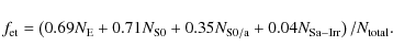
The coefficients in Eq. (4) give the completeness of the quantitative classification in terms of the Desai et al. (2007) visual classes. For example, the adopted B/T and S2 cuts would select 69
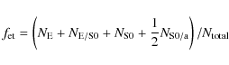
where
It is impossible to recover all the galaxies visually classified as early-types because a visual early-type does not necessarily imply a r1/4 profile. Indeed, many early-type galaxies such as dwarf ellipticals have simple exponential profiles (Lin & Faber 1983; Kormendy 1985), and we have verified through isophote tracing that many galaxies visually classified as early-types and missed by our selection criteria do have radial surface brightness profiles that are exponential and thus consistent with their measured low B/T values.
Table 2: Early-type galaxy fractions based on HST/ACS imaging.
![\begin{figure}
\par\includegraphics[angle=270,width=8.8cm,clip]{78872f3.ps}
\end{figure}](/articles/aa/full_html/2009/48/aa8872-07/img115.png)
|
Figure 3:
Image smoothness parameter S2 versus bulge
fraction B/T for
different visual types. The galaxies selected by our quantitative
early-type galaxy criteria (
|
| Open with DEXTER | |
Given ![]() galaxies brighter than an absolute magnitude limit
galaxies brighter than an absolute magnitude limit
![]() inside a clustercentric radius
inside a clustercentric radius
![]() of which
of which
![]() are early-types galaxies, we actually calculate the early-type galaxy
fraction by finding the median of the binomial probability
distribution
are early-types galaxies, we actually calculate the early-type galaxy
fraction by finding the median of the binomial probability
distribution
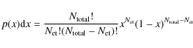
and we integrate Eq. (6) to calculate the lower and upper bounds of the corresponding 68
4.2 HST-based fractions
For each EDisCS cluster with HST/ACS imaging, we have computed the
fraction of early-type galaxies using our quantitative
HST/ACS morphologies (
![]() and and
and and ![]() ). We used
only spectroscopically-confirmed members brighter than an absolute V-band
magnitude
). We used
only spectroscopically-confirmed members brighter than an absolute V-band
magnitude
![]() .
We varied
.
We varied
![]() as a function of redshift from -20.5 at z = 0.8
to -20.1 at z = 0.4 to
account for passive evolution. This choice of
as a function of redshift from -20.5 at z = 0.8
to -20.1 at z = 0.4 to
account for passive evolution. This choice of
![]() was made to be fully consistent with previous work (Poggianti et al. 2006)
although it may not be strictly the best choice for late-type galaxy
populations. Our results did not appear to be sensitive to variations
in
was made to be fully consistent with previous work (Poggianti et al. 2006)
although it may not be strictly the best choice for late-type galaxy
populations. Our results did not appear to be sensitive to variations
in
![]() at the level of a few tens of a magnitude. Following Poggianti et al. (2006),
our early-type galaxy fractions were also computed by weighting each
galaxy according to the incompleteness of the spectroscopic catalog.
This incompleteness depends on both galaxy magnitude and clustercentric
position. Incompleteness as a function of magnitude was computed by
dividing the number of galaxies in the spectroscopic catalog in a given
magnitude bin by the number of galaxies in the parent photometric
catalog in the same bin. We used 0.5 mag bins here.
Incompleteness due to the geometrical effects comes from the finite
number of slitlets per sky area, and the increasing surface density of
galaxies on the sky closer to the cluster centers. Geometric
incompleteness is field dependent as it depends on cluster richness,
and we thus computed this incompleteness on a field-by-field basis. We
also used four radial bins out to R200
with a bin width of 0.25 R200.
at the level of a few tens of a magnitude. Following Poggianti et al. (2006),
our early-type galaxy fractions were also computed by weighting each
galaxy according to the incompleteness of the spectroscopic catalog.
This incompleteness depends on both galaxy magnitude and clustercentric
position. Incompleteness as a function of magnitude was computed by
dividing the number of galaxies in the spectroscopic catalog in a given
magnitude bin by the number of galaxies in the parent photometric
catalog in the same bin. We used 0.5 mag bins here.
Incompleteness due to the geometrical effects comes from the finite
number of slitlets per sky area, and the increasing surface density of
galaxies on the sky closer to the cluster centers. Geometric
incompleteness is field dependent as it depends on cluster richness,
and we thus computed this incompleteness on a field-by-field basis. We
also used four radial bins out to R200
with a bin width of 0.25 R200.
![\begin{figure}
\par\includegraphics[angle=270,width=8.8cm,clip]{78872f4a.ps}\includegraphics[angle=270,width=8.8cm,clip]{78872f4b.ps}
\end{figure}](/articles/aa/full_html/2009/48/aa8872-07/img119.png)
|
Figure 4: Direct galaxy-by-galaxy comparison between bulge fraction ( left-hand panel) and image smoothness ( right-hand panel) measurements from HST/ACS and VLT/FORS2 images. Filled circles are galaxies classified as early-type on both ACS and VLT images, asterisks are galaxies classified as early-type only on the VLT images, pluses are galaxies classified as early-type only on the ACS images, and open circles are galaxies not classified as early-type on either ACS or VLT images, The dashed lines show the cuts used for the definition of an early-type galaxy as discussed in Sects. 4.1 and 4.3. |
| Open with DEXTER | |
The raw and incompleteness-corrected HST-based early-type galaxy
fractions are given in Table 2 for a
maximum clustercentric radius
![]() of 0.6 R200
(Cols. 4 and 5) and R200
(Cols. 9 and 10). Most of the corrected fractions do
not significantly differ from the raw ones because our spectroscopic
sample is essentially complete down to
of 0.6 R200
(Cols. 4 and 5) and R200
(Cols. 9 and 10). Most of the corrected fractions do
not significantly differ from the raw ones because our spectroscopic
sample is essentially complete down to ![]() (
(
![]() -20 at z = 0.8), and we used multiple masks on
dense clusters to improve
the spatial sampling of our spectroscopic sample.
As a comparison, Table 2 also
gives early-type galaxy fractions measured from visual classifications
by Desai et al. (2007)
(Cols. 6 and 7). They should be compared with values
in Col. 5 because cluster galaxy samples selected using
photometric redshifts are de facto free from the magnitude and
geometric incompleteness of our spectroscopic sample. Another important
caveat is that they were computed using two different ways to isolate
cluster members (photometric redshift and statistical background
subtraction), and they are thus not restricted to
spectroscopically-confirmed members. Nonetheless, the agreement
between fractions measured from visual and quantitative classifications
is remarkably good. The largest disagreement is for 1138.2-1133, but
even this case can be considered marginal as it is not quite 2
-20 at z = 0.8), and we used multiple masks on
dense clusters to improve
the spatial sampling of our spectroscopic sample.
As a comparison, Table 2 also
gives early-type galaxy fractions measured from visual classifications
by Desai et al. (2007)
(Cols. 6 and 7). They should be compared with values
in Col. 5 because cluster galaxy samples selected using
photometric redshifts are de facto free from the magnitude and
geometric incompleteness of our spectroscopic sample. Another important
caveat is that they were computed using two different ways to isolate
cluster members (photometric redshift and statistical background
subtraction), and they are thus not restricted to
spectroscopically-confirmed members. Nonetheless, the agreement
between fractions measured from visual and quantitative classifications
is remarkably good. The largest disagreement is for 1138.2-1133, but
even this case can be considered marginal as it is not quite 2![]() .
.
4.3 VLT- versus HST-based fractions
Quantitative morphologies measured from HST images are more robust than
those measured from ground-based images (Sect. 3.2.5 and Simard et al. (2002)).
Figure 4
shows a direct galaxy-by-galaxy comparison between bulge fraction and
image smoothness measurements from HST/ACS and
VLT/FORS2 images. This comparison includes
spectroscopically-confirmed member galaxies from all clusters with
HST imaging that are brighter than
![]() and within a clustercentric radius of 0.6 R200
to take into account the effect of crowding. For a given galaxy, the
agreement between the two sets of measurements will obviously depend on
its apparent
luminosity and size. The overall agreement is reasonably good. The
scatter in the bulge fraction plot is consistent with
and within a clustercentric radius of 0.6 R200
to take into account the effect of crowding. For a given galaxy, the
agreement between the two sets of measurements will obviously depend on
its apparent
luminosity and size. The overall agreement is reasonably good. The
scatter in the bulge fraction plot is consistent with ![]()
![]() 0.1 (Simard et al. 2002)
and
0.1 (Simard et al. 2002)
and ![]()
![]() 0.25 (Fig. 2)
added in quadrature, but the fact that completely independent
segmentation images were used for the HST and
VLT morphological measurements also contributes significantly
to this scatter. Indeed, this scatter would be smaller if only
uncrowded
galaxies (as indicated by the SExtractor photometry flag) on the
VLT images had been plotted here. For the image smoothness
plot, there is a correlation between
0.25 (Fig. 2)
added in quadrature, but the fact that completely independent
segmentation images were used for the HST and
VLT morphological measurements also contributes significantly
to this scatter. Indeed, this scatter would be smaller if only
uncrowded
galaxies (as indicated by the SExtractor photometry flag) on the
VLT images had been plotted here. For the image smoothness
plot, there is a correlation between
![]() and
and
![]() ,
but it is not one-to-one.
,
but it is not one-to-one. ![]() values
increase faster than
values
increase faster than
![]() .
This is expected as PSF blurring will be more
significant on the ground-based images, and S2 measurements
are not corrected for PSF effects. Part of the scatter is
again due to the use of independent
segmentation images.
.
This is expected as PSF blurring will be more
significant on the ground-based images, and S2 measurements
are not corrected for PSF effects. Part of the scatter is
again due to the use of independent
segmentation images.
![\begin{figure}
\par\includegraphics[angle=270,width=8.5cm,clip]{78872f5.ps}
\end{figure}](/articles/aa/full_html/2009/48/aa8872-07/img127.png)
|
Figure 5:
Comparison between early-type galaxy fractions for clusters with
overlapping VLT and HST imaging. VLT/FORS2 and HST/ACS
early-type galaxy fractions were computed using galaxies with |
| Open with DEXTER | |
Table 3: Early-type galaxy fractions based on VLT/FORS2 imaging.
The inclusion of clusters with only VLT/FORS2 imaging allows
us to extend our analysis to nine additional clusters - an
important consideration given that we seek to probe cluster-to-cluster
variations in morphological content. We therefore need to show that we
measure consistent early-type fractions for clusters with overlapping
ACS and FORS2 images. The problem boils down to finding the
set of limits on
![]() and
and
![]() that yield FORS2 early-type fractions in agreement with the
ACS fractions obtained with
that yield FORS2 early-type fractions in agreement with the
ACS fractions obtained with ![]() and
and ![]() when the same galaxies are used for both FORS2 and ACS. For
each cluster, we used all spectroscopically-confirmed cluster members
brighter than
when the same galaxies are used for both FORS2 and ACS. For
each cluster, we used all spectroscopically-confirmed cluster members
brighter than
![]() and within a clustercentric radius of R200.
No corrections for incompleteness were applied here as these
corrections would be identical for both cases. We went through many
manual iterations until we found satisfactory limits on
and within a clustercentric radius of R200.
No corrections for incompleteness were applied here as these
corrections would be identical for both cases. We went through many
manual iterations until we found satisfactory limits on
![]() and
and
![]() .
We found FORS2 fractions to be in very good agreement with the ACS ones
for
.
We found FORS2 fractions to be in very good agreement with the ACS ones
for ![]() and
and ![]() (Fig. 5).
This agreement is especially good if one considers the fact that we
performed our FORS2 and ACS bulge+disk decompositions
completely independently from one another,
i.e., we did not attempt to use the same SExtractor
segmentation map for both FORS2 and HST images. The limit
on
(Fig. 5).
This agreement is especially good if one considers the fact that we
performed our FORS2 and ACS bulge+disk decompositions
completely independently from one another,
i.e., we did not attempt to use the same SExtractor
segmentation map for both FORS2 and HST images. The limit
on
![]() is slightly higher than the one on
is slightly higher than the one on
![]() because lower spatial resolution typically leads to a small
overestimate of the bulge fraction. Similarly, the limit on
because lower spatial resolution typically leads to a small
overestimate of the bulge fraction. Similarly, the limit on
![]() needs to be more stringent than on
needs to be more stringent than on
![]() to select the same galaxies as they will look smoother on the
FORS2 images due to lower resolution.
to select the same galaxies as they will look smoother on the
FORS2 images due to lower resolution.
Following the procedure described in Sect. 4.2, we computed
early-type galaxy fraction for all eighteen clusters using galaxies on
our FORS2 images with ![]() and
and
![]() .
The results are shown in Table 3. The same
incompleteness corrections as in Sect. 4.2 were applied
here as well. The errors on the
early-type galaxy fractions in the table do not include errors
on R200 due to
correlated errors on cluster
.
The results are shown in Table 3. The same
incompleteness corrections as in Sect. 4.2 were applied
here as well. The errors on the
early-type galaxy fractions in the table do not include errors
on R200 due to
correlated errors on cluster ![]() .
We hereafter use our VLT/FORS2 early-type fractions for all
EDisCS clusters for the sake of uniformity.
.
We hereafter use our VLT/FORS2 early-type fractions for all
EDisCS clusters for the sake of uniformity.
4.4 Local clusters
The Sloan Digital Sky Survey (SDSS; Abazajian et al. 2009) offers by far the best, ``local'' (z < 0.1) baseline for a comparison of early-type galaxy fractions between local and high-redshift clusters. Clusters similar in mass to EDisCS clusters can be selected from spectroscopic SDSS data, and galaxy morphologies can be measured using GIM2D from SDSS images. We therefore used SDSS-selected clusters here to construct a local baseline as nearly free of systematics as currently possible given the available data.
We use the sample of SDSS clusters defined in von der Linden (2007).
The basis of this cluster sample is the C4 cluster catalogue (Miller et al. 2005), and
we briefly recapitulate here how the von der Linden et al.
sample was selected. Their primary aim was to find the galaxy closest
to the deepest point of the potential well of a cluster.
In order to insure that the clusters would span a large
angular extent compared to the minimum distance of 55 arcsec
between fibers, the sample was restricted to redshifts ![]() .
This first cut resulted in an initial sample of
833 clusters. A combination of clustercentric
distance, galaxy concentration and colour cuts was used to identify
brightest cluster galaxies (BCGs) for these clusters. For cases where
the same BCG was identified for more than one cluster, only the cluster
with the density peak was retained, and the others were deemed to be
substructures. This cut rejected 101 clusters. Refined
velocity dispersion and virial radii were then computed through an
iterative process of velocity cuts. This process failed for
55 clusters, and these were also rejected. All remaining
clusters were then visually inspected. An additional set of
35 clusters were rejected at this point as being in the infall
regions of other clusters, and another 17 clusters were
discarded because they had less than three galaxies within 3
.
This first cut resulted in an initial sample of
833 clusters. A combination of clustercentric
distance, galaxy concentration and colour cuts was used to identify
brightest cluster galaxies (BCGs) for these clusters. For cases where
the same BCG was identified for more than one cluster, only the cluster
with the density peak was retained, and the others were deemed to be
substructures. This cut rejected 101 clusters. Refined
velocity dispersion and virial radii were then computed through an
iterative process of velocity cuts. This process failed for
55 clusters, and these were also rejected. All remaining
clusters were then visually inspected. An additional set of
35 clusters were rejected at this point as being in the infall
regions of other clusters, and another 17 clusters were
discarded because they had less than three galaxies within 3![]() of the cluster redshift and 1 R200
of its center. This brought the total of SDSS clusters down
to 625. Following Poggianti
et al. (2006), we applied a final redshift cut to
keep clusters in the range 0.04 < z
< 0.085. The lower limit reduces fiber aperture effects, and the
upper limit minimizes incompleteness in galaxy absolute magnitude. Our
final SDSS comparison sample thus has 439 clusters.
of the cluster redshift and 1 R200
of its center. This brought the total of SDSS clusters down
to 625. Following Poggianti
et al. (2006), we applied a final redshift cut to
keep clusters in the range 0.04 < z
< 0.085. The lower limit reduces fiber aperture effects, and the
upper limit minimizes incompleteness in galaxy absolute magnitude. Our
final SDSS comparison sample thus has 439 clusters.
Given that we are interested in probing galaxy properties as a
function of environment, it is important to ensure that the
SDSS and EDisCS samples both cover the same range of
environments. We therefore selected a subsample of
SDSS clusters with a velocity dispersion distribution matching
the EDisCS distribution. This match was done by adding
SDSS clusters to the subsample one at a time and keeping only
those that maintained the EDisCS-SDSS two-sample Kolmogorov-Smirnov
probability above 50![]() .
This is the probability of the maximum difference between the
normalized cumulative distributions of the EDisCS and
SDSS samples. It means that even if the two sampls were
selected at random from the same underlying distribution, they would
differ by more than the two observed samples more than half the time.
This probability threshold thus yields a SDSS subsample that
is very well-matched to the EDisCS clusters. The resulting
subsample (referred to as ``SDSS-C4'' hereafter) includes
158 clusters, and these clusters are listed
in Table 4.
.
This is the probability of the maximum difference between the
normalized cumulative distributions of the EDisCS and
SDSS samples. It means that even if the two sampls were
selected at random from the same underlying distribution, they would
differ by more than the two observed samples more than half the time.
This probability threshold thus yields a SDSS subsample that
is very well-matched to the EDisCS clusters. The resulting
subsample (referred to as ``SDSS-C4'' hereafter) includes
158 clusters, and these clusters are listed
in Table 4.
We ran GIM2D on SDSS Data Release Seven (DR7; Abazajian et al. 2009)
u-, g-, r-
and i-band images of objects in the magnitude range
14 ![]()
![]()
![]() 17.77 with a galaxy spectrum (i.e., with field
SpecClass = 2 in database table SpecPhoto).
Bulge+disk decompositions were successfully obtained for
674 693 galaxies (Simard, in preparation).
GIM2D morphologies for galaxies in our matched
SDSS-C4 clusters were extracted from this large morphological
database to compute early-type fractions. There are two sources of
incompleteness that must be taken into account here. The first one is
incompleteness versus magnitude. We denote this spectroscopic
completeness function as
17.77 with a galaxy spectrum (i.e., with field
SpecClass = 2 in database table SpecPhoto).
Bulge+disk decompositions were successfully obtained for
674 693 galaxies (Simard, in preparation).
GIM2D morphologies for galaxies in our matched
SDSS-C4 clusters were extracted from this large morphological
database to compute early-type fractions. There are two sources of
incompleteness that must be taken into account here. The first one is
incompleteness versus magnitude. We denote this spectroscopic
completeness function as
![]() here, and we compute it around each cluster position
by taking the ratio of the number of galaxies in the spectroscopic
SDSS catalog (database table SpecPhoto) to the number of
galaxies in the photometric SDSS catalog (database table PhotoPrimary)
as a function of Petrosian r magnitude.
Galaxies around a given position on the sky were extracted from the
database using the SDSS ``fGetNearbyObjEq'' function. The second source
of incompleteness
comes from the spatial sampling of the SDSS fibers on the sky.
Fibers cannot be placed closer than 55
here, and we compute it around each cluster position
by taking the ratio of the number of galaxies in the spectroscopic
SDSS catalog (database table SpecPhoto) to the number of
galaxies in the photometric SDSS catalog (database table PhotoPrimary)
as a function of Petrosian r magnitude.
Galaxies around a given position on the sky were extracted from the
database using the SDSS ``fGetNearbyObjEq'' function. The second source
of incompleteness
comes from the spatial sampling of the SDSS fibers on the sky.
Fibers cannot be placed closer than 55
![]() from one another. This means that regions with a higher surface density
of targets could not be sampled as completely as regions in the global
field. The net result for SDSS clusters is a decrease in
spectroscopic sampling as a function of decreasing clustercentric
distance R. We can map the
spectroscopic completeness versus R by
computing the ratio of galaxies in the spectroscopic and photometric
SDSS catalogs as a function of R.
We denote this geometrical completeness function as
from one another. This means that regions with a higher surface density
of targets could not be sampled as completely as regions in the global
field. The net result for SDSS clusters is a decrease in
spectroscopic sampling as a function of decreasing clustercentric
distance R. We can map the
spectroscopic completeness versus R by
computing the ratio of galaxies in the spectroscopic and photometric
SDSS catalogs as a function of R.
We denote this geometrical completeness function as
![]() here. Ideally,
here. Ideally, ![]() should be computed for each cluster because it will depend on cluster
richness and apparent size (and thus indirectly on redshift).
However, in practice, there are not enough galaxies in a single cluster
to yield
should be computed for each cluster because it will depend on cluster
richness and apparent size (and thus indirectly on redshift).
However, in practice, there are not enough galaxies in a single cluster
to yield
![]() with acceptable error bars. So, we opted for averaging clusters with
the same redshifts and velocity dispersions to compute
with acceptable error bars. So, we opted for averaging clusters with
the same redshifts and velocity dispersions to compute
![]() .
We divided the cluster list of Table 4 into three
cluster groups: (1) z < 0.06;
(2) z > 0.06,
.
We divided the cluster list of Table 4 into three
cluster groups: (1) z < 0.06;
(2) z > 0.06, ![]() km s-1;
and (3) z > 0.06,
km s-1;
and (3) z > 0.06, ![]() km s-1.
The weight
km s-1.
The weight
![]() in the spectroscopic catalog of a galaxy with a r'-band
magnitude m at a clustercentric R
is thus given by the product
in the spectroscopic catalog of a galaxy with a r'-band
magnitude m at a clustercentric R
is thus given by the product ![]() ,
and the completeness-weighted early-fraction of a SDSS cluster
is then simply:
,
and the completeness-weighted early-fraction of a SDSS cluster
is then simply:
![$\displaystyle %
\tiny {
f_{\rm et}\left (
\begin{array}{c}
M_{V}\leq-19.8, \\
...
..._{V}\leq-19.8, \\
R\leq R_{\rm et}]
\end{array}} W_{\rm spec}(m_i,R_i)}}\cdot}$](/articles/aa/full_html/2009/48/aa8872-07/img139.png)
In terms of spatial resolution, the ACS, SDSS and FORS2 images have sampling of 0.68 kpc/FWHM at z = 0.8 (0
![\begin{figure}
\par\includegraphics[angle=270,width=8.8cm,clip]{78872f6.ps}
\end{figure}](/articles/aa/full_html/2009/48/aa8872-07/img144.png)
|
Figure 6:
Comparison between fractions of [OII] emitters computed using
emission-line measurements from Brinchmann
et al. (2004) and the DR7 release. Filled
and open circles are clusters with |
| Open with DEXTER | |
The raw fractions of [OII] emitters for the 158 SDSS-C4
clusters were calculated by directly querying the
SDSS database table SpecLine for the [OII]3727 and [OII]3730
equivalent widths for each confirmed cluster member, adding them
together and correcting them to rest-frame by dividing by (1+z).
The corrected [OII] fractions were then computed following
exactly the same calculations (and using the same weights, the same
luminosity and clustercentric radius cuts of ![]() and
and ![]() )
as for the early-type fractions except that the early-type selection
criteria on bulge fraction and image smoothness were simply replaced by
the Poggianti et al.
(2006) cut of EW([OII])
)
as for the early-type fractions except that the early-type selection
criteria on bulge fraction and image smoothness were simply replaced by
the Poggianti et al.
(2006) cut of EW([OII]) ![]()
![]() .
In order to evaluate the importance of the errors on our equivalent
widths on our determination of the fractions of
[OII] emitters, we also computed [OII] fractions
using equivalent widths from Brinchmann
et al. (2004). The two sets of equivalent widths are
plotted against one another in Fig. 6. The
agreement between the two sets is excellent, and we conclude that our
[OII] fractions are robust.
.
In order to evaluate the importance of the errors on our equivalent
widths on our determination of the fractions of
[OII] emitters, we also computed [OII] fractions
using equivalent widths from Brinchmann
et al. (2004). The two sets of equivalent widths are
plotted against one another in Fig. 6. The
agreement between the two sets is excellent, and we conclude that our
[OII] fractions are robust.
Table 4
gives corrected early-type galaxy fractions and fractions of
[OII] computed for ![]() for the 158 SDSS clusters in our local comparison
sample. We included only galaxies brighter than
for the 158 SDSS clusters in our local comparison
sample. We included only galaxies brighter than
![]() to avoid incompleteness in the SDSS spectroscopic sample. This
cutoff magnitude corresponds to the absolute magnitude limits we used
for our distant EDisCS clusters once passive evolution is
taken into account (see Sect. 4.2).
to avoid incompleteness in the SDSS spectroscopic sample. This
cutoff magnitude corresponds to the absolute magnitude limits we used
for our distant EDisCS clusters once passive evolution is
taken into account (see Sect. 4.2).
![\begin{figure}
\par\includegraphics[angle=90,width=7.75cm,clip]{78872f7a.ps}\hsp...
...*{1.15cm}
\includegraphics[angle=90,width=7.55cm,clip]{78872f7d.ps}
\end{figure}](/articles/aa/full_html/2009/48/aa8872-07/img149.png)
|
Figure 7:
Early-type galaxies in Millennium Simulation dark matter haloes
Top, left-hand panel: early-type galaxy fraction within
0.6 R200 versus
cluster velocity dispersion at three different redshifts.
Top, right-hand panel: early-type galaxy fraction within
0.6 R200 versus
age of the universe. Blue and red points are clusters with velocity
dispersions below and above 600 km s-1
respectively. Lower, left-hand panel: early-type
galaxy fraction within
0.6 R200 versus
fraction of star-forming galaxies in clusters with |
| Open with DEXTER | |
4.5 Theoretical models
Numerical simulations of dark matter haloes populated with galaxies
using semi-analytical models greatly help in the interpretation of
observational results. We use here the Millennium Simulation (MS; Springel et al. 2005),
and the semi-analytical code described in De
Lucia & Blaizot (2007)![]() .
The MS followed 21603 particles of mass
8.6
.
The MS followed 21603 particles of mass
8.6 ![]() 10
10
![]() within a comoving box of size 500 h-1 Mpc
on a side with a spatial resolution of 5 h-1 kpc.
Early-type galaxy fractions were computed from these simulated galaxy
catalogs using the following procedure. Haloes were randomly selected
at three different redshifts (z = 0, 0.41,
0.62) so that they were uniformly distributed in log(M200).
The final halo sample was 100 haloes at z =
0, 94 haloes at z = 0.41 and
92 haloes at z = 0.62.
For each of these haloes, all galaxies in a cubic box 6 Mpc on
a side around the central galaxy were selected, and a morphological
type was assigned to each model galaxy by computing the quantity
within a comoving box of size 500 h-1 Mpc
on a side with a spatial resolution of 5 h-1 kpc.
Early-type galaxy fractions were computed from these simulated galaxy
catalogs using the following procedure. Haloes were randomly selected
at three different redshifts (z = 0, 0.41,
0.62) so that they were uniformly distributed in log(M200).
The final halo sample was 100 haloes at z =
0, 94 haloes at z = 0.41 and
92 haloes at z = 0.62.
For each of these haloes, all galaxies in a cubic box 6 Mpc on
a side around the central galaxy were selected, and a morphological
type was assigned to each model galaxy by computing the quantity ![]() =
= ![]() (in the rest-frame B-band). Galaxies with
(in the rest-frame B-band). Galaxies with ![]() <
1.0 were considered to be ``early-type''. This is the same criterion as
selecting real galaxies with
<
1.0 were considered to be ``early-type''. This is the same criterion as
selecting real galaxies with ![]() .
It is important here to note that an early-type galaxy in the
simulations was defined solely based on this cut in bulge fraction
because the simulations do not have the resolution required to model
internal fine structures such as asymmetries. Given that real,
early-type galaxies were also selected according to image smoothness,
one might find the early-type fractions of real clusters to be
systematically lower. For each halo, the fraction of early-type
galaxies within 0.6 R200
from the BCG was computed using three different projections.
Furthermore, only galaxies that were within 2 Mpc from the BCG along
the line of sight were included. The fractions were computed using only
galaxies brighter than -20.5, -20.1, and -19.8 in the
rest-frame V-band at redshift 0.6, 0.4,
and 0.0 respectively to match the limits used for the SDSS and
EDisCS early-type galaxy fractions. A galaxy in the simulation
was deemed to be star-forming if its star-formation rate in the last
timestep of its evolution was not equal to zero.
.
It is important here to note that an early-type galaxy in the
simulations was defined solely based on this cut in bulge fraction
because the simulations do not have the resolution required to model
internal fine structures such as asymmetries. Given that real,
early-type galaxies were also selected according to image smoothness,
one might find the early-type fractions of real clusters to be
systematically lower. For each halo, the fraction of early-type
galaxies within 0.6 R200
from the BCG was computed using three different projections.
Furthermore, only galaxies that were within 2 Mpc from the BCG along
the line of sight were included. The fractions were computed using only
galaxies brighter than -20.5, -20.1, and -19.8 in the
rest-frame V-band at redshift 0.6, 0.4,
and 0.0 respectively to match the limits used for the SDSS and
EDisCS early-type galaxy fractions. A galaxy in the simulation
was deemed to be star-forming if its star-formation rate in the last
timestep of its evolution was not equal to zero.
![\begin{figure}
\par\includegraphics[angle=270,width=8.8cm,clip]{78872f8a.ps}\includegraphics[angle=270,width=8.8cm,clip]{78872f8b.ps}
\end{figure}](/articles/aa/full_html/2009/48/aa8872-07/img153.png)
|
Figure 8:
Early-type galaxy fraction within
0.6 R200 versus
velocity dispersion for SDSS and EDisCS clusters. Both samples
have been matched in velocity dispersion. Left panel:
SDSS clusters. Only typical error bars are shown in the lower
right-hand corner for clarity. Right panel: filled
and open circles are mid-z and high-z
EDisCS clusters respectively. Errors bars shown in both panels
are 1 |
| Open with DEXTER | |
Figure 7
shows the resulting model early-type fractions as a function of cluster
velocity dispersion, redshift and fraction of star-forming galaxies for
the MS haloes. At a given redshift, there is no
dependence of the early-type fraction on cluster velocity dispersion,
but the scatter symmetrically increases towards both lower and higher
fractions leading to a ``wedge-like'' distribution towards lower
cluster ![]() 's.
The early-type fractions of both low and high-mass clusters increase
with decreasing redshift from
's.
The early-type fractions of both low and high-mass clusters increase
with decreasing redshift from ![]() 0.70 at z = 0.65 to
0.70 at z = 0.65 to ![]() 0.85 at z = 0.
The early-type fractions of massive clusters are anticorrelated with
the fractions of star-forming galaxies: clusters at z
= 0 have higher early-type fractions but lower fractions of
star-forming galaxies. Note that the trends in Fig. 7 do not
agree with those shown in Diaferio
et al. (2001) although the assumptions made about
morphological transformations are very similar in the two models.
In particular, the MS shows little trend of early-type
fraction with cluster velocity dispersion but a substantial trend with
redshift, while Diaferio et al. found the opposite. This is
likely a result of the poorer mass resolution, poorer statistics and
cruder dynamical modelling of the earlier paper.
0.85 at z = 0.
The early-type fractions of massive clusters are anticorrelated with
the fractions of star-forming galaxies: clusters at z
= 0 have higher early-type fractions but lower fractions of
star-forming galaxies. Note that the trends in Fig. 7 do not
agree with those shown in Diaferio
et al. (2001) although the assumptions made about
morphological transformations are very similar in the two models.
In particular, the MS shows little trend of early-type
fraction with cluster velocity dispersion but a substantial trend with
redshift, while Diaferio et al. found the opposite. This is
likely a result of the poorer mass resolution, poorer statistics and
cruder dynamical modelling of the earlier paper.
5 Results
We use here our VLT/FORS2 early-type fractions for all EDisCS clusters for the sake of uniformity.5.1 Early-type galaxy fractions versus cluster velocity dispersion and redshift
Figure 8 shows early-type galaxy fractions versus velocity dispersion for the SDSS and EDisCS clusters. The early-type galaxy fractions of both cluster samples exhibit no clear trend as a function ofFigure 8 does
show that there is a marked difference in the morphological content of
the EDisCS and SDSS clusters. All EDisCS ![]() values
(with the exception of one cluster) are below 0.6, but half of
the SDSS clusters are above this value. The population of early-type
galaxies has thus increased significantly in half of the clusters of
all velocity dispersions. An increase in early-type
fraction with decreasing redshift may already be visible when one
compares mid-z and high-z EDisCS
clusters. Mid-z clusters around
values
(with the exception of one cluster) are below 0.6, but half of
the SDSS clusters are above this value. The population of early-type
galaxies has thus increased significantly in half of the clusters of
all velocity dispersions. An increase in early-type
fraction with decreasing redshift may already be visible when one
compares mid-z and high-z EDisCS
clusters. Mid-z clusters around ![]() =
500 km s-1 have
=
500 km s-1 have ![]()
![]() 0.5 whereas the high-z clusters have
0.5 whereas the high-z clusters have ![]()
![]() 0.4.
This would represent a
0.4.
This would represent a ![]() 25
25![]() increase over a time interval of 2 Gyr. As shown in
Fig. 7,
the early-type fractions of clusters in the Millenium Simulation also
increase with decreasing redshift in clusters of all velocity
dispersions, but there is a lack of simulated clusters with
increase over a time interval of 2 Gyr. As shown in
Fig. 7,
the early-type fractions of clusters in the Millenium Simulation also
increase with decreasing redshift in clusters of all velocity
dispersions, but there is a lack of simulated clusters with ![]() compared with the SDSS-C4 clusters. The scatter in the
compared with the SDSS-C4 clusters. The scatter in the ![]() values
of simulated clusters is also smaller than in those of real clusters.
For simulated clusters at z = 0 with
values
of simulated clusters is also smaller than in those of real clusters.
For simulated clusters at z = 0 with ![]()
![]() 600 km s-1,
600 km s-1, ![]() = 0.06
compared to
= 0.06
compared to ![]() = 0.21
for SDSS clusters over the same range of velocity dispersions.
Given that the mean error on the SDSS
= 0.21
for SDSS clusters over the same range of velocity dispersions.
Given that the mean error on the SDSS ![]() values
is 0.12, the intrinsic scatter would be 0.17. This
intrinsic scatter is still almost three times the scatter in the
simulated clusters.
values
is 0.12, the intrinsic scatter would be 0.17. This
intrinsic scatter is still almost three times the scatter in the
simulated clusters.
Table 5: Spearman rank test results for early-type fraction versus cluster velocity dispersion.
![\begin{figure}
\par\includegraphics[angle=270,width=8.8cm,clip]{78872f9a.ps}\includegraphics[angle=270,width=8.8cm,clip]{78872f9b.ps}
\end{figure}](/articles/aa/full_html/2009/48/aa8872-07/img158.png)
|
Figure 9:
Early-type galaxy fraction versus age of the universe (i.e., redshift)
for clusters with |
| Open with DEXTER | |
Figure 9
shows SDSS and EDisCS early-type fractions as a function of the age of
the universe (i.e., redshift). The clusters have been divided
into two subgroups based on their velocity dispersions. The early-type
fractions of massive (![]() >
600 km s-1)
EDisCS clusters (right panel) are in very good agreement with
the ones in the compilation of van
Dokkum et al. (2001) which also have velocity
dispersions greater than 600 km s-1.
The clusters at low redshift in the van
Dokkum et al. (2001) compilation suggest that there
are no local clusters with low early-type fractions and hence that all
clusters have uniformly increased their early-type fraction from
>
600 km s-1)
EDisCS clusters (right panel) are in very good agreement with
the ones in the compilation of van
Dokkum et al. (2001) which also have velocity
dispersions greater than 600 km s-1.
The clusters at low redshift in the van
Dokkum et al. (2001) compilation suggest that there
are no local clusters with low early-type fractions and hence that all
clusters have uniformly increased their early-type fraction from ![]() to the present day. However, our SDSS cluster sample shows that this
simple picture is not entirely true. While half of the SDSS clusters
have higher early-type fractions than clusters at high redshift, the
other half have early-type fractions equal or even lower than the
EDisCS clusters. The same holds true for the low mass clusters
(left-hand panel). The scatter in
to the present day. However, our SDSS cluster sample shows that this
simple picture is not entirely true. While half of the SDSS clusters
have higher early-type fractions than clusters at high redshift, the
other half have early-type fractions equal or even lower than the
EDisCS clusters. The same holds true for the low mass clusters
(left-hand panel). The scatter in
![]() (<0.1) in high-mass EDisCS clusters does appear to be
considerably less that the scatter seen in low-mass clusters.
(<0.1) in high-mass EDisCS clusters does appear to be
considerably less that the scatter seen in low-mass clusters.
The lack of a clear trend in early-type fraction with redshift in the right-hand panel of Fig. 9 is in disagreement with the Millennium Simulation prediction in the top right-hand panel of Fig. 7. There is a clear deficit of clusters with low early-type fraction at low redshift in the Millenium Simulation compared with our SDSS sample.
5.2 Early-type galaxy fractions versus fractions of [OII] emitters
The link between star formation and morphological transformation and
its evolution as a function of redshift provides more clues on the
processes driving galaxy morphology in local and distant
clusters. The fractions of galaxies with [OII] emission in the
EDisCS clusters were computed as in Poggianti
et al. (2006) using the same absolute magnitude
limits and the same prescriptions for correcting magnitude and
geometric incompletness, but the clustercentric radius cut was changed
to match the one used for the early-type fractions in this paper (
![]() ).
The two datasets are therefore directly comparable. Figure 10 shows
).
The two datasets are therefore directly comparable. Figure 10 shows ![]() versus
versus
![]() with our local and distant samples again divided according to velocity
dispersion. Table 7 gives
Spearman test results between
with our local and distant samples again divided according to velocity
dispersion. Table 7 gives
Spearman test results between
![]() and
and
![]() .
There is a strong correlation between
.
There is a strong correlation between ![]() versus
versus
![]() in both SDSS and EDisCS cluster samples irrespective of
cluster velocity dispersion. The EDisCS clusters lie within
the envelopes defined by the SDSS clusters. There is no offset
between the zeropoints of the correlations at low and high redshift.
However, as demonstrated by
Poggianti et al. (2006),
the star formation activity (parametrized by
in both SDSS and EDisCS cluster samples irrespective of
cluster velocity dispersion. The EDisCS clusters lie within
the envelopes defined by the SDSS clusters. There is no offset
between the zeropoints of the correlations at low and high redshift.
However, as demonstrated by
Poggianti et al. (2006),
the star formation activity (parametrized by
![]() )
has decreased in all environments from
)
has decreased in all environments from ![]() to
to ![]() .
This is confirmed by the K-S test results in Table 8. The
probabilities that the EDisCS and SDSS clusters are drawn from
the same parent
.
This is confirmed by the K-S test results in Table 8. The
probabilities that the EDisCS and SDSS clusters are drawn from
the same parent ![]() distribution
are only 0.026, 0.005 and 0.046 for the whole
samples, low
distribution
are only 0.026, 0.005 and 0.046 for the whole
samples, low ![]() and high
and high ![]() subsamples respectively.
subsamples respectively.
The ![]() versus
versus ![]() values for clusters from the Millenium Simulation (Fig. 7) are
quite different from the observations. Low
values for clusters from the Millenium Simulation (Fig. 7) are
quite different from the observations. Low ![]() MS clusters at low and high redshifts are confined to
high
MS clusters at low and high redshifts are confined to
high
![]() and
and ![]() values with no
apparent correlation. There is only a handful of clusters with low
values for both
values with no
apparent correlation. There is only a handful of clusters with low
values for both
![]() and
and
![]() .
The high
.
The high ![]() MS clusters are found in a very limited range of
MS clusters are found in a very limited range of
![]() and
and ![]() values (
values (
![]() ,
,
![]() ).
).
![\begin{figure}
\par\includegraphics[angle=270,width=8.8cm,clip]{78872f10a.ps}\includegraphics[angle=270,width=8.8cm,clip]{78872f10b.ps}
\end{figure}](/articles/aa/full_html/2009/48/aa8872-07/img166.png)
|
Figure 10:
Early-type galaxy fraction versus [OII] emitter fraction for
clusters with |
| Open with DEXTER | |
6 Discussion
In order to fully understand possible evolutionary trends observed
here, it is important to determine how cluster velocity
dispersion changes with redshift as a result of the hierarchical growth
of structures. Are we looking at similar clusters when we focus on the
same range of velocity dispersions in the SDSS and
EDisCS clusters? Poggianti
et al. (2006) looked at the mean change in ![]() between z = 0 and z = 0.76
using a sample of 90 haloes from the Millennium Simulation
uniformly distributed in log(mass) between 5
between z = 0 and z = 0.76
using a sample of 90 haloes from the Millennium Simulation
uniformly distributed in log(mass) between 5 ![]() 1012 and 5
1012 and 5 ![]() 10
10
![]() .
Their Fig. 8
shows how
.
Their Fig. 8
shows how ![]() evolves over that redshift interval. For example, a z =
0 cluster with
evolves over that redshift interval. For example, a z =
0 cluster with ![]() =
900 km s-1 would typically
have
=
900 km s-1 would typically
have ![]() 750 km s-1 at z = 0.76.
This evolution is not sufficient to introduce biases in our analysis
here. Indeed, selecting clusters with
750 km s-1 at z = 0.76.
This evolution is not sufficient to introduce biases in our analysis
here. Indeed, selecting clusters with ![]() 600 km s-1, say, at either z = 0
or z = 0.76 would keep nearly all the same
clusters. Measured velocity dispersions may exhibit a large scatter
with respect to the true halo mass particularly for low-mass clusters.
The velocity dispersions for the SDSS and EDisCS clusters were
calculated in a very similar way in order to minimize any biases.
Velocity dispersions calculated from a small number of cluster members
may be overestimates of the true cluster mass. Table 1 lists
1103.7-1245b as the cluster with the lowest number of members (N = 11).
In order to check the robustness of our results, we re-ran our analyses
by excluding SDSS clusters in Table 4 with N
< 10 for which velocity dispersions may be less reliable and
found that our results remained unchanged.
600 km s-1, say, at either z = 0
or z = 0.76 would keep nearly all the same
clusters. Measured velocity dispersions may exhibit a large scatter
with respect to the true halo mass particularly for low-mass clusters.
The velocity dispersions for the SDSS and EDisCS clusters were
calculated in a very similar way in order to minimize any biases.
Velocity dispersions calculated from a small number of cluster members
may be overestimates of the true cluster mass. Table 1 lists
1103.7-1245b as the cluster with the lowest number of members (N = 11).
In order to check the robustness of our results, we re-ran our analyses
by excluding SDSS clusters in Table 4 with N
< 10 for which velocity dispersions may be less reliable and
found that our results remained unchanged.
Table 6: Two-sample Kolmogorov-Smirnov test probabilities for early-type fraction versus cluster velocity dispersion.
Table 7: Spearman rank test results for early-type fraction versus fraction of [OII] emitters.
Table 8: Two-sample Kolmogorov-Smirnov test probabilities for [OII] emitter fraction versus cluster velocity dispersion.
Poggianti et al.
(2006) proposed a scenario in which two channels are
responsible for the production of passive galaxies in clusters, and
others (Faber
et al. 2007; Brown et al. 2007) have
proposed a similar scenario for the migration of galaxies from the
``blue cloud'' to the red sequence. ``Primordial passive galaxies'' are
composed of galaxies whose stars all formed at very high redshift (z
> 2) over a short timescale. These galaxies have been observed
in clusters up and beyond z = 1, and they largely
comprise luminous ellipticals. ``Quenched passive galaxies'' have had a
more extended period of star formation activity, and their star
formation has been quenched after their infall into dense cluster
environments. These quenched passive galaxies would then suffer the
effects of cluster processes such as ram pressure stripping,
harassment, strangulation and mergers to become S0 and earlier type
galaxies. A key point of this scenario is that processes
affecting morphology and star formation activity operate on different
timescales as shown recently for the EDisCS sample by Sánchez-Blázquez et al. (2009).
There is good evidence that star formation is quenched in galaxies over
timescales of 1-3 Gyr after they have entered the cluster
environment (Poggianti
et al. 2006,1999) whereas morphological
transformation through mergers and harassment can take longer (![]() 5 Gyr,
Moore et al. 1998).
The best example of this is the fact that the vast majority of
post-starburst galaxies in distant clusters, those that have had their
star formation activity terminated during the last Gyr, still
retain a spiral morphology (Poggianti
et al. 1999). Such a two-channel scenario would
naturally explain observations indicating that the elliptical galaxy
fraction actually remains constant with redshift while the
S0 fraction rises with decreasing redshift (Fasano
et al. 2000; Desai et al. 2007; Dressler
et al. 1997). Unfortunately, the
VLT/FORS2 images do not have sufficient spatial resolution to
disentangle E and S0 galaxies as mentioned in Sect. 4.1 to determine
the exact contribution from each channel. We can therefore only study
the overall production of early-type galaxies, but it should exhibit
different behaviors with cluster global properties depending on the
process(es) dominating it. Given our quantitative definition of an
early-type galaxy based on bulge fraction and image smoothness, there
are essentially two ways to transform late-type galaxies into
early-type ones: 1) processes such as collisions and
harassment that can fundamentally alter the structure of a galaxy by
forming bulges and/or destroying disks and 2) quenching
processes that can extinguish star forming regions responsible for some
of the galaxy image asymmetries and also cause a fading of
the disks.
5 Gyr,
Moore et al. 1998).
The best example of this is the fact that the vast majority of
post-starburst galaxies in distant clusters, those that have had their
star formation activity terminated during the last Gyr, still
retain a spiral morphology (Poggianti
et al. 1999). Such a two-channel scenario would
naturally explain observations indicating that the elliptical galaxy
fraction actually remains constant with redshift while the
S0 fraction rises with decreasing redshift (Fasano
et al. 2000; Desai et al. 2007; Dressler
et al. 1997). Unfortunately, the
VLT/FORS2 images do not have sufficient spatial resolution to
disentangle E and S0 galaxies as mentioned in Sect. 4.1 to determine
the exact contribution from each channel. We can therefore only study
the overall production of early-type galaxies, but it should exhibit
different behaviors with cluster global properties depending on the
process(es) dominating it. Given our quantitative definition of an
early-type galaxy based on bulge fraction and image smoothness, there
are essentially two ways to transform late-type galaxies into
early-type ones: 1) processes such as collisions and
harassment that can fundamentally alter the structure of a galaxy by
forming bulges and/or destroying disks and 2) quenching
processes that can extinguish star forming regions responsible for some
of the galaxy image asymmetries and also cause a fading of
the disks.
Applying the Poggianti
et al. (2006) scenario to our results, the
``threshold'' in ![]() values
in our high redshift clusters (Figs. 8
and 9)
could be explained by a population of primordial passive galaxies that
formed at even higher redshifts. Most of our high redshift clusters
have early-type fractions in the range 0.3-0.6 with no correlation with
cluster velocity dispersion. Are these early-type fractions indeed
consistent with a populations of primordial passive galaxies?
Calculations done in Poggianti
et al. (2006) show that the fraction of galaxies at z
= 0.6 that were present in haloes with masses greater than 3
values
in our high redshift clusters (Figs. 8
and 9)
could be explained by a population of primordial passive galaxies that
formed at even higher redshifts. Most of our high redshift clusters
have early-type fractions in the range 0.3-0.6 with no correlation with
cluster velocity dispersion. Are these early-type fractions indeed
consistent with a populations of primordial passive galaxies?
Calculations done in Poggianti
et al. (2006) show that the fraction of galaxies at z
= 0.6 that were present in haloes with masses greater than 3 ![]() 10
10
![]() at z = 2.5 is 0.4
at z = 2.5 is 0.4 ![]() 0.2. These primordial passive galaxies can therefore account
for at least 2/3 (if not all) of the early-type
populations in high redshift clusters, and their high formation
redshift would explain the lack of dependence of
0.2. These primordial passive galaxies can therefore account
for at least 2/3 (if not all) of the early-type
populations in high redshift clusters, and their high formation
redshift would explain the lack of dependence of
![]() on cluster velocity dispersion.
on cluster velocity dispersion.
One of our main results is that the early-type fractions of
galaxy clusters increase from z
= 0.6-0.8 to ![]() in clusters of all velocity dispersions. What kind of morphological
transformation process(es) can lead to such an evolution? Collisions
and harassment both depend on galaxy-galaxy interactions and the time a
galaxy has spent within the cluster environment. Cluster velocity
dispersion influences the number of interactions and their duration.
Higher velocity dispersions in more massive clusters yield more
interactions per unit time N but with
shorter durations
in clusters of all velocity dispersions. What kind of morphological
transformation process(es) can lead to such an evolution? Collisions
and harassment both depend on galaxy-galaxy interactions and the time a
galaxy has spent within the cluster environment. Cluster velocity
dispersion influences the number of interactions and their duration.
Higher velocity dispersions in more massive clusters yield more
interactions per unit time N but with
shorter durations ![]() in a given time interval. One might therefore expect to see a peak in
early-type type fraction at the cluster velocity dispersion where the
product
in a given time interval. One might therefore expect to see a peak in
early-type type fraction at the cluster velocity dispersion where the
product
![]() is maximized. No such peak is seen in our clusters.
Ram-pressure stripping is expected to go as (
is maximized. No such peak is seen in our clusters.
Ram-pressure stripping is expected to go as (
![]() (Gaetz et al. 1987)
with
(Gaetz et al. 1987)
with
![]() ,
,
![]() and
and
![]() being the density of the ICM, the velocity of the galaxies within the
ICM and the rate at which galaxies can replenish their gas
respectively. The fraction of passive galaxies should therefore be a
relatively strong function of cluster velocity dispersion if quenching
by ram pressure stripping is the dominant process. The number of
post-starburst galaxies in EDisCS clusters does correlate with
cluster velocity dispersion (Poggianti
et al. 2009a), but the uniform increase in
early-type fractions at all cluster velocity dispersions observed going
from EDisCS to SDSS clusters is not consistent with the
intracluster medium being the main cause of the changes in cluster
morphological content.
being the density of the ICM, the velocity of the galaxies within the
ICM and the rate at which galaxies can replenish their gas
respectively. The fraction of passive galaxies should therefore be a
relatively strong function of cluster velocity dispersion if quenching
by ram pressure stripping is the dominant process. The number of
post-starburst galaxies in EDisCS clusters does correlate with
cluster velocity dispersion (Poggianti
et al. 2009a), but the uniform increase in
early-type fractions at all cluster velocity dispersions observed going
from EDisCS to SDSS clusters is not consistent with the
intracluster medium being the main cause of the changes in cluster
morphological content.
Even though the EDisCS and SDSS early-type fractions show no
correlation with cluster velocity dispersion, and the SDSS
[OII] emitter fractions (but not the EDisCS ones) also show no
such correlation (Poggianti
et al. 2006; Popesso et al. 2007),
there is a very strong correlation between
![]() and
and
![]() .
This correlation is seen at both low and high cluster masses as well as
at both low and high redshifts. Morphology and star formation therefore
appear to be closely linked with one another over a wide range of
environments and times. However, different structural transformation
and quenching processes are thought to operate over different
timescales (e.g., Sánchez-Blázquez
et al. 2009). Timescales range from 1-2 Gyr
(based on typical cluster crossing times) for truncating star formation
to 3-5 Gyr for totally extinguishing star formation in newly
accreted galaxies (Poggianti
et al. 2006; Tonnesen & Bryan 2009).
Looking at the evolution of EDisCS cluster red-sequence
galaxies over 2 Gyr (from z = 0.75 to z
= 0.45), Sánchez-Blázquez
et al. (2009) found that morphological
transformation and quenching of star formation indeed appeared to not
be simultaneous. As noted in Sect. 5.1, the
early-type fractions of mid-z
EDisCS clusters may be
.
This correlation is seen at both low and high cluster masses as well as
at both low and high redshifts. Morphology and star formation therefore
appear to be closely linked with one another over a wide range of
environments and times. However, different structural transformation
and quenching processes are thought to operate over different
timescales (e.g., Sánchez-Blázquez
et al. 2009). Timescales range from 1-2 Gyr
(based on typical cluster crossing times) for truncating star formation
to 3-5 Gyr for totally extinguishing star formation in newly
accreted galaxies (Poggianti
et al. 2006; Tonnesen & Bryan 2009).
Looking at the evolution of EDisCS cluster red-sequence
galaxies over 2 Gyr (from z = 0.75 to z
= 0.45), Sánchez-Blázquez
et al. (2009) found that morphological
transformation and quenching of star formation indeed appeared to not
be simultaneous. As noted in Sect. 5.1, the
early-type fractions of mid-z
EDisCS clusters may be ![]() 25
25![]() higher than the ones of high-z clusters. This change
would therefore have taken place over a 2 Gyr
interval in our adopted cosmology. However, the time baseline here
between SDSS and EDisCS clusters is almost 6 Gyr,
and, unfortunately, this is ample time to erase any difference arising
from different timescales in the link between morphology and star
formation.
higher than the ones of high-z clusters. This change
would therefore have taken place over a 2 Gyr
interval in our adopted cosmology. However, the time baseline here
between SDSS and EDisCS clusters is almost 6 Gyr,
and, unfortunately, this is ample time to erase any difference arising
from different timescales in the link between morphology and star
formation.
The lack of dependence of morphology and star formation on global cluster properties such as velocity dispersion raises the question of whether changes in galaxy properties are driven by more local effects or whether they occur outside of the cluster environment. Recent work (Bamford et al. 2009; Poggianti et al. 2008; Park & Choi 2009; Ellison et al. 2009) have re-emphasized the strong link between galaxy properties and local galaxy density rather than cluster membership. Galaxy properties are seen to change at densities around 15-40 galaxies Mpc-2 or projected separations of 20-30 h-1 kpc. Others (e.g., Wilman et al. 2009; Kautsch et al. 2008) have suggested that the galaxy group environment might be more conducive to galaxy transformation. Our observed evolution in early-type fraction as a function of redshift and the strong correlation between morphology and star formation at all cluster masses would support the idea that cluster membership is of lesser importance than other variables such as local density in determining galaxy properties.
The properties of simulated clusters from the Millenium
Simulation compare well with those of EDisCS and
SDSS clusters. Their early-type fractions also show no
dependence with cluster velocity dispersion in contrast to previous
theoretical work (e.g. Diaferio
et al. 2001) but in agreement with observations.
However, there is a definite lack of MS clusters with low
early-type fractions at z = 0
compared to the SDSS sample. It is important here to note that
an early-type galaxy in the simulations was defined solely based on its
bulge fraction because the simulations do not have the resolution
required to model internal fine structures such as asymmetries. Given
that real, early-type galaxies were also selected according to image
smoothness, one would expect the early-type fractions of real clusters
to be systematically lower. However, half of the SDSS clusters
have low early-type fractions not seen in the simulations at z = 0,
and such a large discrepancy could only be explained by a significant
population of real bulge-dominated galaxies with relatively large
asymmetries. It is more likely that bulge formation in the
simulations may be too efficient. The scatter in ![]() values
for the simulated clusters with
values
for the simulated clusters with ![]()
![]() 600 km s-1 is also nearly
three times smaller than observed in the real clusters (Sect. 5.1) which may
indicate that the models may not include the right mixture of
evolutionary processes at work on real galaxies. High-mass simulated
clusters show a correlation between early-type fraction and
star-forming fraction (albeit over narrower ranges than observed), but
the correlation is not seen in the low-mass simulated clusters. This
may be understood by high mass clusters having been formed long enough
for evolutionary processes to have had enough time to act on galaxies
to modify their properties whereas this is not necessarily the case for
low-mass clusters. The fact that the correlation is observed in both
low- and high-mass real clusters may be an indication that processes
giving rise to the correlation may be more efficient
(or altogether different) than modelled. It is also
important to keep in mind here that the properties of a galaxy in these
models are essentially driven by the mass of its parent halo.
600 km s-1 is also nearly
three times smaller than observed in the real clusters (Sect. 5.1) which may
indicate that the models may not include the right mixture of
evolutionary processes at work on real galaxies. High-mass simulated
clusters show a correlation between early-type fraction and
star-forming fraction (albeit over narrower ranges than observed), but
the correlation is not seen in the low-mass simulated clusters. This
may be understood by high mass clusters having been formed long enough
for evolutionary processes to have had enough time to act on galaxies
to modify their properties whereas this is not necessarily the case for
low-mass clusters. The fact that the correlation is observed in both
low- and high-mass real clusters may be an indication that processes
giving rise to the correlation may be more efficient
(or altogether different) than modelled. It is also
important to keep in mind here that the properties of a galaxy in these
models are essentially driven by the mass of its parent halo.
7 Summary
We have presented quantitative morphologies measured from PSF-convolved, 2D bulge+disk decompositions of cluster and field galaxies on deep VLT/FORS2 images of eighteen, optically-selected galaxy clusters at 0.45 < z < 0.80 observed as part of the ESO Distant Cluster Survey. The morphological content of these clusters was characterized by the early-type fraction within a clustercentric radius of 0.6 R200, and early-type galaxies were selected based on bulge fraction and image smoothness. We showed a very good agreement between quantitative and visual galaxy classifications. We used a set of 158 clusters extracted from the Sloan Digital Sky Survey matched in velocity dispersion to our EDisCS sample and analyzed exactly in the same way to provide a robust comparison baseline and to control systematics. We studied trends in early-type fraction as a function of cluster mass and redshift. We also explored the link between morphology and star formation by comparing early-type fractions to the fractions of [OII] emitters in our clusters. Our main results are:
- 1.
- The early-type fractions of the SDSS and EDisCS clusters exhibit no clear trend as a function of cluster velocity dispersion.
- 2.
- Mid-z EDisCS clusters around
 =
500 km s-1 have
=
500 km s-1 have 
 0.5 whereas high-z EDisCS clusters have
0.4. This represents a
0.5 whereas high-z EDisCS clusters have
0.4. This represents a  25
25 increase over a time interval of 2 Gyr.
- 3.
- There is a marked difference in the morphological content of the EDisCS and SDSS samples. None of the EDisCS clusters have an early-type fraction greater than 0.6 whereas half of the SDSS clusters lie above this value. This difference is seen in clusters of all velocity dispersions (i.e., masses).
- 4.
- There is a strong and clear correlation between morphology and star formation activity in the sense that decreasing fractions of [OII] emitters are tracked by increasing early-type fractions. This correlation holds in both low and high cluster masses as well as at both low and high redshift.
- 5.
- The early-type fractions of clusters drawn from the Millennium Simulation (Springel et al. 2005) using the galaxy formation model of De Lucia & Blaizot (2007) also show no clear dependence on cluster velocity dispersion. However, at z = 0, they are not enough simulated clusters with low early-type fractions compared to the SDSS cluster sample. While high-mass simulated clusters show a correlation between early-type fraction and star-forming fraction (albeit over narrower ranges than observed), this correlation is not seen in the low-mass simulated clusters in contrast to the real ones.
We are thankful to the anonymous referee for suggestions that greatly contributed this paper. We have benefitted from the generosity of the ESO/OPC. G.R. thanks Special Research Area No 375 of the German Research Foundation for financial support. The Millennium Simulation databases used in this paper and the web applications providing access to them were constructed as part of the activities of the German Astrophysical Virtual Observatory. Funding for the creation and distribution of the SDSS Archive has been provided by the Alfred P. Sloan Foundation, the Participating Institutions, the National Aeronautics and Space Administration, the National Science Foundation, the US Department of Energy, the Japanese Monbukagakusho, and the Max Planck Society. The SDSS Web site is http://www.sdss.org/. The SDSS is managed by the Astrophysical Research Consortium (ARC) for the Participating Institutions. The Participating Institutions are The University of Chicago, Fermilab, the Institute for Advanced Study, the Japan Participation Group, The Johns Hopkins University, the Korean Scientist Group, Los Alamos National Laboratory, the Max-Planck-Institute for Astronomy (MPIA), the Max-Planck-Institute for Astrophysics (MPA), New Mexico State University, University of Pittsburgh, University of Portsmouth, Princeton University, the United States Naval Observatory, and the University of Washington. The Dark Cosmology Centre is funded by the Danish National Research Foundation.
References
- Abazajian, K., Adelman-McCarthy, J. K., Agüeros, M. A., et al. 2009, ApJS, 182, 543 [NASA ADS] [CrossRef]
- Allen, S. W. 1998, MNRAS, 296, 392 [NASA ADS] [CrossRef]
- Andredakis, Y. C. 1998, MNRAS, 295, 725 [NASA ADS] [CrossRef]
- Balcells, M., Graham, A. W., Domínguez-Palmero, L., & Peletier, R. E. 2003, ApJ, 582, 79 [NASA ADS] [CrossRef]
- Bamford, S. P., Nichol, R. C., Baldry, I. K., et al. 2009, MNRAS, 393, 1324 [NASA ADS] [CrossRef]
- Barnes, J. E., & Hernquist, L. 1992, ARA&A, 30, 705 [NASA ADS] [CrossRef]
- Barnes, J. E., & Hernquist, L. 1996, ApJ, 471, 115 [NASA ADS] [CrossRef]
- Barazza, F. D., Jablonka, P., Desai, V., et al. 2009, A&A, 497, 713 [NASA ADS] [EDP Sciences] [CrossRef]
- Bessell, M. S. 1990, PASP, 102, 1181 [NASA ADS] [CrossRef]
- Bertin, E., & Arnouts, S. 1996, A&AS, 117, 393 [NASA ADS] [EDP Sciences] [CrossRef]
- Blakeslee, J. P., Holden, B. P., Franx, M., et al. 2006, ApJ, 644, 30 [NASA ADS] [CrossRef]
- Borgani, S., Girardi, M., Carlberg, R. G., Yee, H. K. C., & Ellingson, E. 1999, ApJ, 527, 561 [NASA ADS] [CrossRef]
- Brinchmann, J., Charlot, S., White, S. D. M., et al. 2004, MNRAS, 351, 1151 [NASA ADS] [CrossRef]
- Brown, M. J. I., Dey, A., Jannuzi, B. T., et al. 2007, ApJ, 654, 858 [NASA ADS] [CrossRef]
- Carlberg, R. G., Yee, H. K. C., & Ellingson, E. 1997, ApJ, 478, 462 [NASA ADS] [CrossRef]
- Clowe, D., Schneider, P., Aragón-Salamanca, A., et al. 2006, A&A, 451, 395 [NASA ADS] [EDP Sciences] [CrossRef]
- Courteau, S., de Jong, R. S., & Broeils, A. H. 1996, ApJ, 457, 73 [NASA ADS] [CrossRef]
- de Jong, R. S. 1996, A&A, 118, 557 [CrossRef]
- De Lucia, G., & Blaizot, J. 2007, MNRAS, 375, 2 [NASA ADS] [CrossRef]
- De Lucia, G., Poggianti, B. M., Aragón-Salamanca, A., et al. 2004, ApJ, 610, 77 [NASA ADS] [CrossRef]
- De Lucia, G., Poggianti, B. M., Aragón-Salamanca, A., et al. 2007, MNRAS, 374, 809 [NASA ADS] [CrossRef]
- Desai, V., Dalcanton, J. J., Aragón-Salamanca, A., et al. 2007, ApJ, 660, 1151 [NASA ADS] [CrossRef]
- Diaferio, A., Kauffmann, G., Balogh, M. L., et al. 2001, MNRAS, 323, 999 [NASA ADS] [CrossRef]
- Dressler, A. 1984, ApJ, 281, 512 [NASA ADS] [CrossRef]
- Dressler, A., Oemler, A., Jr., Couch, W. J., et al. 1997, ApJ, 490, 577 [NASA ADS] [CrossRef]
- Ellison, S. L., Simard, L., Cowan, N. B., et al. 2009, MNRAS, 396, 1257 [NASA ADS] [CrossRef]
- Faber, S. M., Willmer, C. N. A., Wolf, C., et al. 2007, ApJ, 665, 265 [NASA ADS] [CrossRef]
- Farouki, R. T., & Shapiro, S. L. 1981, ApJ, 243, 32 [NASA ADS] [CrossRef]
- Farouki, R. T., & Shapiro, S. L. 1982, ApJ, 259, 103 [NASA ADS] [CrossRef]
- Fasano, G., Poggianti, B., Couch, W. J., et al. 2000, ApJ, 542, 673 [NASA ADS] [CrossRef]
- Finn, R. A., Zaritsky, D., McCarthy, D. W. Jr., et al. 2005, ApJ, 630, 206 [NASA ADS] [CrossRef]
- Fukugita, M., Nakamura, O., Okamura, S., et al. 2007, AJ, 134, 579 [NASA ADS] [CrossRef]
- Gaetz, T. J., Salpeter, E. E., & Shaviv, G. 1987, ApJ, 316, 530 [NASA ADS] [CrossRef]
- Gladders, M. D., & Yee, H. K. C. 2005, ApJS, 157, 1 [NASA ADS] [CrossRef]
- Gonzalez, A. H., Zaritsky, D., Dalcanton, J. J., & Nelson, A. 2001, ApJS, 137, 117 [NASA ADS] [CrossRef]
- Gonzalez, A. H., Zaritsky, D., Simard, L., Clowe, D., & White, S. D. M. 2002, ApJ, 579, 577 [NASA ADS] [CrossRef]
- Gunn, J. E., & Gott, J. R. I. 1972, ApJ, 176, 1 [NASA ADS] [CrossRef]
- Halliday, C., Milvang-Jensen, B., Poirier, S., et al. 2004, A&A, 427, 397 [NASA ADS] [EDP Sciences] [CrossRef]
- Hoekstra, H., Franx, M., & Kuijken, K. 2000, ApJ, 532, 88 [NASA ADS] [CrossRef]
- Holden, B. P., Stanford, S. A., Eisenhardt, P., & Dickinson, M. 2004, ApJ, 127, 2484 [NASA ADS]
- Holden, B. P., Illingworth, G. D., Franx, M., et al. 2007, ApJ, 670, 190 [NASA ADS] [CrossRef]
- Holden, B. P., Franx, M., Illingworth, G. D., et al. 2009, ApJ, 693, 617 [NASA ADS] [CrossRef]
- Im, M., Simard, L., Faber, S. M., et al. 2002, ApJ, 571, 136 [NASA ADS] [CrossRef]
- Johnson, O., Best, P., Zaritsky, D., et al. 2006, MNRAS, 371, 1777 [NASA ADS] [CrossRef]
- Kaiser, N., & Squires, G. 1993, ApJ, 404, 441 [NASA ADS] [CrossRef]
- Kautsch, S. J., Gonzalez, A. H., Soto, C. A., et al. 2008, ApJ, 688, 5 [NASA ADS] [CrossRef]
- Kormendy, J. 1985, ApJ, 295, 73 [NASA ADS] [CrossRef]
- Lane, K. P., Gray, M. E., Aragón-Salamanca, A., Wolf, C., & Meisenheimer, K. 2007, MNRAS, 378, 716 [NASA ADS] [CrossRef]
- Lanzoni, B., Guiderdoni, B., Mamon, G. A., Devriendt, J., & Hatton, S. 2005, MNRAS, 361, 369 [NASA ADS] [CrossRef]
- Larson, R. B., Tinsley, B. M., & Caldwell, C. N. 1980, ApJ, 237, 692 [NASA ADS] [CrossRef]
- Lin, D. N. C., & Faber, S. M. 1983, ApJ, 266, 17 [CrossRef]
- Lubin, L. M., Oke, J. B., & Postman, M. 2002, AJ, 124, 1905 [NASA ADS] [CrossRef]
- Martig, M., Bournaud, F., Teyssier, R., & Dekel, A. 2009, ApJ, submitted
- McIntosh, D. H., Rix, H.-W., & Caldwell, N. 2002, ApJ, 610, 161 [NASA ADS] [CrossRef]
- Milvang-Jensen, B., Noll, S., Halliday, C., et al. 2008, A&A, 482, 419 [NASA ADS] [EDP Sciences] [CrossRef]
- Mihos, J., & Hernquist, L. 1996, ApJ, 464, 641 [NASA ADS] [CrossRef]
- Miller, C. J., Nichol, R. C., Reichart, D., et al. 2005, AJ, 130, 968 [NASA ADS] [CrossRef]
- Moran, S. M., Ellis, R. S., Treu, T., et al. 2007, ApJ, 671, 1503 [NASA ADS] [CrossRef]
- Moore, B., Katz, N., Lake, G., Dressler, A., & Oemler, A. 1996, Nature, 379, 613 [NASA ADS] [CrossRef]
- Moore, B., Lake, G., & Katz, N. 1998, ApJ, 495, 139 [NASA ADS] [CrossRef]
- Negroponte, J., & White, S. D. M. 1983, MNRAS, 205, 1009 [NASA ADS]
- Park, C., & Choi, Y.-Y. 2009, ApJ, 691, 1828 [NASA ADS] [CrossRef]
- Pelló, R., et al. 2009, A&A, in press
- Poggianti, B. M., Smail, I., Dressler, A., et al. 1999, ApJ, 518, 576 [NASA ADS] [CrossRef]
- Poggianti, B. M., von der Linden, A., De Lucia, G., et al. 2006, ApJ, 642, 188 [NASA ADS] [CrossRef]
- Poggianti, B. M., Desai, V., Finn, R., et al. 2008, ApJ, 684, 888 [NASA ADS] [CrossRef]
- Poggianti, B. M., Aragón-Salamanca, A., Zaritsky, D., et al. 2009a, ApJ, 693, 112 [NASA ADS] [CrossRef]
- Poggianti, B. M., Fasano, G., Bettoni, D., et al. 2009b, ApJ, 697, L137 [NASA ADS] [CrossRef]
- Popesso, P., Biviano, A., Romaniello, M., & Böhringer, H. 2007, A&A, 461, 411 [NASA ADS] [EDP Sciences] [CrossRef]
- Postman, M., Franx, M., Cross, N. J. G., et al. 2005, ApJ, 623, 721 [NASA ADS] [CrossRef]
- Quilis, V., Moore, B., & Bower, R. 2000, Science, 288, 1617 [NASA ADS] [CrossRef]
- Rood, H. J., Page, T. L., Kintner, E. C., & King, I. R. 1972, ApJ, 175, 627 [NASA ADS] [CrossRef]
- Rudnick, G., von der Linden, A., Pelló, R., et al. 2009, ApJ, 700, 1559 [NASA ADS] [CrossRef]
- Sánchez-Blázquez, P., Jablonka, P., Noll, S., et al. 2009, A&A, 499, 47 [NASA ADS] [EDP Sciences] [CrossRef]
- Schneider, P., & Seitz, C. 1995, A&A, 294, 411 [NASA ADS]
- Simard, L., Willmer, C. N. A., Vogt, N. P., et al. 2002, ApJS, 142, 1 [NASA ADS] [CrossRef]
- Smith, G. P., Treu, T., Ellis, R. S., Moran, S. M., & Dressler, A. 2005, ApJ, 620, 78 [NASA ADS] [CrossRef]
- Spitzer, L. J., & Baade, W. 1951, ApJ, 113, 413 [NASA ADS] [CrossRef]
- Springel, V., White, S. D. M., Jenkins, A., et al. 2005, Nature, 435, 629 [NASA ADS] [CrossRef]
- Steinmetz, M., & Navarro, J. F. 2002, New Astron., 7, 155 [NASA ADS] [CrossRef]
- Stetson, P. B. 1987, PASP, 99, 191 [NASA ADS] [CrossRef]
- Tonnesen, S., & Bryan, G. L. 2009, ApJ, 694, 789 [NASA ADS] [CrossRef]
- Toomre, A., & Toomre, J. 1972, ApJ, 178, 623 [NASA ADS] [CrossRef]
- Tran, K.-V. H., Kelson, D. D., van Dokkum, P., et al. 1999, ApJ, 522, 39 [NASA ADS] [CrossRef]
- Tran, K.-V. H., Simard, L., Illingworth, G. D., & Franx, M. 2003, ApJ, 590, 238 [NASA ADS] [CrossRef]
- van der Wel, A., Holden, B. P., Franx, M., et al. 2007, ApJ, 670, 206 [NASA ADS] [CrossRef]
- van Dokkum, P. G., Franx, M., Fabricant, D., Illingworth, G. D., & Kelson, D. D. 2000, ApJ, 541, 95 [NASA ADS] [CrossRef]
- van Dokkum, P. G., Stanford, S. A., Holden, B. P., et al. 2001, ApJ, 552, 101 [NASA ADS] [CrossRef]
- von der Linden, A., Best, P. N., Kauffmann, G., & White, S. D. M. 2007, MNRAS, 379, 867 [NASA ADS] [CrossRef]
- White, S. D. M., Clowe, D. I., Simard, L., et al. 2005, A&A, 444, 365 [NASA ADS] [EDP Sciences] [CrossRef]
- Willis, J. P., Pacaud, F., Valtchanov, I., et al. 2005, MNRAS, 363, 675 [NASA ADS] [CrossRef]
- Wilman, D. J., Oemler, A., Mulchaey, J. S., et al. 2009, ApJ, 692, 298 [NASA ADS] [CrossRef]
- Wolf, C., Gray, M. E., Aragón-Salamanca, A., Lane, K. P., & Meisenheimer, K. 2007, MNRAS, 376, L1 [NASA ADS] [CrossRef]
- Zabludoff, A. I., & Mulchaey, J. S. 1998, ApJ, 496, 39 [NASA ADS] [CrossRef]
Online Material
Table 4: Velocity-dispersion-matched sample of 158 SDSS clusters in order of decreasing velocity dispersion.
Footnotes
- ... 0.8
- Based on observations obtained in visitor and service modes at the ESO Very Large Telescope (VLT) as part of the Large Programme 166.A-0162 (the ESO Distant Cluster Survey). Also based on observations made with the NASA/ESA Hubble Space Telescope, obtained at the Space Telescope Science Institute, which is operated by the Association of Universities for Research in Astronomy, Inc., under NASA contract NAS 5-26555. These observations are associated with proposal 9476. Support for this proposal was provided by NASA through a grant from the Space Telescope Science Institute.
- ...
- Table 4 is only available in electronic form at http://www.aanda.org
- ... IRAF
- IRAF is distributed by the National Optical Astronomy Observatories, which are operated by the Association of Universities for Research in Astronomy, Inc., under cooperative agreement with the National Science Foundation.
- ...De Lucia & Blaizot (2007)
- Simulated galaxy catalogs used here are publicly available at http://www.mpa-garching.mpg.de/millennium/
All Tables
Table 1: Main characteristics of the EDisCS cluster sample.
Table 2: Early-type galaxy fractions based on HST/ACS imaging.
Table 3: Early-type galaxy fractions based on VLT/FORS2 imaging.
Table 5: Spearman rank test results for early-type fraction versus cluster velocity dispersion.
Table 6: Two-sample Kolmogorov-Smirnov test probabilities for early-type fraction versus cluster velocity dispersion.
Table 7: Spearman rank test results for early-type fraction versus fraction of [OII] emitters.
Table 8: Two-sample Kolmogorov-Smirnov test probabilities for [OII] emitter fraction versus cluster velocity dispersion.
Table 4: Velocity-dispersion-matched sample of 158 SDSS clusters in order of decreasing velocity dispersion.
All Figures
|
|
Figure 1:
Two-dimensional maps of GIM2D systematic and random galaxy magnitude
and half-light radius errors from 2000 VLT/FORS2 image
simulations. Top left-hand panel: systematic error
on recovered galaxy total magnitude
|
| Open with DEXTER | |
| In the text | |
|
|
Figure 2:
Two-dimensional maps of GIM2D systematic and random galaxy bulge
fraction errors from 2000 VLT/FORS2 image simulations.
Top left-hand panel: systematic error on recovered galaxy
bulge fraction
|
| Open with DEXTER | |
| In the text | |
|
|
Figure 3:
Image smoothness parameter S2 versus bulge
fraction B/T for
different visual types. The galaxies selected by our quantitative
early-type galaxy criteria (
|
| Open with DEXTER | |
| In the text | |
|
|
Figure 4: Direct galaxy-by-galaxy comparison between bulge fraction ( left-hand panel) and image smoothness ( right-hand panel) measurements from HST/ACS and VLT/FORS2 images. Filled circles are galaxies classified as early-type on both ACS and VLT images, asterisks are galaxies classified as early-type only on the VLT images, pluses are galaxies classified as early-type only on the ACS images, and open circles are galaxies not classified as early-type on either ACS or VLT images, The dashed lines show the cuts used for the definition of an early-type galaxy as discussed in Sects. 4.1 and 4.3. |
| Open with DEXTER | |
| In the text | |
|
|
Figure 5:
Comparison between early-type galaxy fractions for clusters with
overlapping VLT and HST imaging. VLT/FORS2 and HST/ACS
early-type galaxy fractions were computed using galaxies with |
| Open with DEXTER | |
| In the text | |
|
|
Figure 6:
Comparison between fractions of [OII] emitters computed using
emission-line measurements from Brinchmann
et al. (2004) and the DR7 release. Filled
and open circles are clusters with |
| Open with DEXTER | |
| In the text | |
|
|
Figure 7:
Early-type galaxies in Millennium Simulation dark matter haloes
Top, left-hand panel: early-type galaxy fraction within
0.6 R200 versus
cluster velocity dispersion at three different redshifts.
Top, right-hand panel: early-type galaxy fraction within
0.6 R200 versus
age of the universe. Blue and red points are clusters with velocity
dispersions below and above 600 km s-1
respectively. Lower, left-hand panel: early-type
galaxy fraction within
0.6 R200 versus
fraction of star-forming galaxies in clusters with |
| Open with DEXTER | |
| In the text | |
|
|
Figure 8:
Early-type galaxy fraction within
0.6 R200 versus
velocity dispersion for SDSS and EDisCS clusters. Both samples
have been matched in velocity dispersion. Left panel:
SDSS clusters. Only typical error bars are shown in the lower
right-hand corner for clarity. Right panel: filled
and open circles are mid-z and high-z
EDisCS clusters respectively. Errors bars shown in both panels
are 1 |
| Open with DEXTER | |
| In the text | |
|
|
Figure 9:
Early-type galaxy fraction versus age of the universe (i.e., redshift)
for clusters with |
| Open with DEXTER | |
| In the text | |
|
|
Figure 10:
Early-type galaxy fraction versus [OII] emitter fraction for
clusters with |
| Open with DEXTER | |
| In the text | |
Copyright ESO 2009
Current usage metrics show cumulative count of Article Views (full-text article views including HTML views, PDF and ePub downloads, according to the available data) and Abstracts Views on Vision4Press platform.
Data correspond to usage on the plateform after 2015. The current usage metrics is available 48-96 hours after online publication and is updated daily on week days.
Initial download of the metrics may take a while.