| Issue |
A&A
Volume 508, Number 3, December IV 2009
|
|
|---|---|---|
| Page(s) | 1469 - 1483 | |
| Section | The Sun | |
| DOI | https://doi.org/10.1051/0004-6361/200912455 | |
| Published online | 27 October 2009 | |
A&A 508, 1469-1483 (2009)
Formation of Ellerman bombs due to 3D flux emergence
V. Archontis - A. W. Hood
School of Mathematics and Statistics, University of St. Andrews, North Haugh, St. Andrews, Fife, KY16 9SS, UK
Received 8 May 2009 / Accepted 21 October 2009
Abstract
Aims. We investigate the emergence of a ``sea-serpent''
magnetic field into the outer solar atmosphere and the connection
between undulating fieldlines and formation of Ellerman bombs.
Methods. We perform 3D numerical experiments solving the time-dependent and resistive MHD equations.
Results. A sub-photospheric magnetic flux sheet develops
undulations due to the Parker instability. It rises from the
convectively unstable sub-photospheric layer and emerges into the
highly stratified atmosphere through successive reconnection events
along the undulating system. Brightenings with the characteristics of
Ellerman bombs are produced due to reconnection, which occurs during
the emergence of the field. At an advanced stage of the evolution of
the system, the resistive emergence leads to the formation of long,
arch-like magnetic fields that expand into the corona. The enhancement
of the magnetic field at the low atmosphere and episodes of emergence
of new magnetic flux are also discussed.
Key words: Sun: magnetic fields - Sun: corona - magnetohydrodynamics (MHD) - methods: numerical - Sun: activity
1 Introduction
The emergence of magnetic flux from the solar interior leads to the appearance of emerging flux regions (EFRs)
when the rising field intersects the visible surface of the Sun. A typical model for flux emergence relies on the
buoyant rise of a sub-photospheric flux tube, which adopts an ![]() -like shape through the process of emergence.
A classical bipolar active region may form as a result of the intersection of the
-like shape through the process of emergence.
A classical bipolar active region may form as a result of the intersection of the ![]() -loop
with the photosphere (Zwaan 1985). EFRs may also appear as growing arch-filament systems in H
-loop
with the photosphere (Zwaan 1985). EFRs may also appear as growing arch-filament systems in H![]() or as a
system of coronal loops recorded in UV when the emerging fieldlines expand into the outer solar atmosphere.
or as a
system of coronal loops recorded in UV when the emerging fieldlines expand into the outer solar atmosphere.
On the other hand, high-resolution observations suggest that the photospheric distribution of emerging magnetic flux
in active regions can be interpreted in terms of multiple undulations. Pariat et al. (2004) applied a linear force-free extrapolation to these
observational data and found that the EFR possessed a hierarchy of small undulating loops, overlaid by larger
loops that may account for arch filament systems. The general geometry of the system consists of a series of connected ![]() and
and ![]() segments
that form an overall ``sea-serpent'' configuration of an emerging field.
segments
that form an overall ``sea-serpent'' configuration of an emerging field.
The ``sea-serpent'' topology was first suggested by Harvey & Harvey (1973) to explain the undulating pattern of moving magnetic features near sunspots. Although there is no detailed explanation for this phenomenon yet, many observations are consistent with the ``sea-serpent'' model. Bernasconi et al. (2002) reported on the structure of moving dipolar features when new magnetic flux was emerging in an active region and showed that they appeared as undulations in the emerging field. They suggested that moving dipolar features are, in fact, U-loops or flux ropes with a concave-downward shape that are tied to the photosphere by trapped mass. A process by which these fields could escape through the solar surface has been proposed by Spruit et al. (1987).
An interesting result of the work by Pariat et al. (2007)
was that the undulatory magnetic flux system seemed to be connected to
the photosphere by bald patches (BPs). BPs are associated with
fieldlines having dips tangent to the photosphere and, thus, it is
likely to be related with the ![]() segments of the undulating field. In general, they are located over an inversion line (Bz=0) where the magnetic field
has a positive curvature
segments of the undulating field. In general, they are located over an inversion line (Bz=0) where the magnetic field
has a positive curvature
![]() .
If the same condition is satisfied for heights above the photosphere, then the
region possesses a magnetic dip. The criterion for the existence of BPs was first given by Seehafer (1986) and later on, in more detail by Titov & Démoulin (1999).
Dipped magnetic field configurations have been studied by Mackay et al. (1999) and Mackay & van Ballegooijen (2009).
.
If the same condition is satisfied for heights above the photosphere, then the
region possesses a magnetic dip. The criterion for the existence of BPs was first given by Seehafer (1986) and later on, in more detail by Titov & Démoulin (1999).
Dipped magnetic field configurations have been studied by Mackay et al. (1999) and Mackay & van Ballegooijen (2009).
Fieldlines that go through BPs belong to quasi-separatrix surfaces where current layers may develop, leading to occurrence of reconnection. Thus, BPs appear to be preferential sites of reconnection and possible sites of heating enhancement. Mandrini et al. (2002) found that some arch filament systems and surges, which were linked with flux emergence in a short-lived active region, were also associated with BPs. They also showed that current layers can be formed at BPs, detected in this active region, and efficiently dissipated in the chromosphere.
Pariat et al. (2004) studied the magnetic
topology of serpentine-like emerging field lines and found that there
is a close connection between BPs and the location of Ellerman bombs
(EBs), which are small-scale brightenings and brief emissions in the
wings of the
![]() line.
EBs were firstly observed by Ellerman (1917) and have been detected mainly within active regions. They have been observed in regions of emerging flux
(between the two main polarities) and also in regions that surround isolated sunspots (Socas-Navarro et al. 2006).
line.
EBs were firstly observed by Ellerman (1917) and have been detected mainly within active regions. They have been observed in regions of emerging flux
(between the two main polarities) and also in regions that surround isolated sunspots (Socas-Navarro et al. 2006).
The observations by Pariat et al. (2004) and Georgoulis et al. (2002) correspond to the central region of an emerging active region. Based on these observations Pariat et al. (2004) proposed a resistive flux emergence model where EBs are connected with low-lying fieldlines with a serpentine shape. Then, coronal loops in active regions and long flux systems (e.g. arch filament systems) may appear due to the rise of undulating magnetic fields that they reconnect at BPs. These loops get rid of the over-dense photospheric plasma by reconnection at BPs. The brightenings at the regions where reconnection occurs may account for the observational appearance of EBs (Pariat et al. 2004; Ding et al. 1998; Georgoulis et al. 2002; Fang et al. 2006). The undulatory shape of the rising magnetic field and the reconnection at the low atmosphere may also be used for the explanation of moving magnetic features and the EBs observed surrounding sunspots.
The wavelength of the undulations of the ``sea-serpent'' field has been
found to be larger than 2 Mm. From a set of identified serpentine
lines in their model, Pariat et al. (2004) found that the distance between successive EBs along the undulating flux tubes has a peak around 3 Mm and a cutoff for
values smaller than 2 Mm. Watanabe et al. (2008) reported that magnetic fields around EBs are undulatory with a characteristic wavelength of ![]() 4 Mm. These sizes
are larger than the convective scales for granulation (
4 Mm. These sizes
are larger than the convective scales for granulation (![]() 1 Mm) or less than supergranulation (
1 Mm) or less than supergranulation (![]() 10 Mm) and are indicative of the presence of some
instability.
10 Mm) and are indicative of the presence of some
instability.
The Parker instability (Parker 1966) may develop at the interface between the emerging flux system and the isothermal photosphere. The interface is
subject to the instability when a perturbation of some wavenumber ![]() is imposed on the lighter (compared to the surrounding plasma) but more
magnetized flux system. For large wavenumbers, the instability is
inhibited by the magnetic tension of the highly curved fieldlines.
However, quantitative estimates have shown that there is a critical
wavelength below which the magnetic tension is not able to prevent the
triggering of the instability. One finds that, using a typical value
for the temperature at the photosphere (
is imposed on the lighter (compared to the surrounding plasma) but more
magnetized flux system. For large wavenumbers, the instability is
inhibited by the magnetic tension of the highly curved fieldlines.
However, quantitative estimates have shown that there is a critical
wavelength below which the magnetic tension is not able to prevent the
triggering of the instability. One finds that, using a typical value
for the temperature at the photosphere (![]() 5800 K), an undulating flux system will be
Parker-unstable if the wavelength of the undulations is
5800 K), an undulating flux system will be
Parker-unstable if the wavelength of the undulations is
![]() Mm. Nozawa et al. (1992) who studied the linear and non-linear properties of the Parker instability
in a convectively unstable layer has confirmed the above results. Also, Shibata et al. (1989)
performed 2D MHD simulations showing that a sub-photospheric horizontal
flux sheet is unstable to the undular mode of the Parker instability
and forms a rising magnetic loop that expands into the corona. The most
unstable wavelength for the fastest growing mode is
Mm. Nozawa et al. (1992) who studied the linear and non-linear properties of the Parker instability
in a convectively unstable layer has confirmed the above results. Also, Shibata et al. (1989)
performed 2D MHD simulations showing that a sub-photospheric horizontal
flux sheet is unstable to the undular mode of the Parker instability
and forms a rising magnetic loop that expands into the corona. The most
unstable wavelength for the fastest growing mode is ![]()
![]() ,
where
,
where
![]() is the pressure scale height at the photosphere.
is the pressure scale height at the photosphere.
The above theoretical considerations and observations suggest that undulations in a magnetic flux system may develop due to the Parker instability. The further emergence of the magnetic field is subject to the magnetic buoyancy instability and the process of reconnection along the serpentine field lines. The first numerical experiments, which were performed to study the evolution of an undulatory magnetic field due to the Parker instability were 2D and reported by Isobe et al. (2007). They found that magnetic reconnection in the lower solar atmosphere could explain the main characteristics of EBs, such as temperature and density enhancement. They also reported on the formation of long magnetic flux systems in the higher atmosphere and the formation of surge-like structures at low atmospheric heights due to reconnection.
In this paper, we present the results of the first three-dimensional model of resistive flux emergence of an undulating flux system. We focus on two main aspects of the problem: firstly, the way the field is emerging into the corona, leaving the dense plasma in the low atmosphere, and forming large-scale flux systems into the corona and secondly, how small-scale brightenings, with the characteristics of EBs, are triggered during the emergence of the field. We also report on other events such as the intensification of the photospheric magnetic field and new episodes of magnetic flux emergence.
The layout of the present paper is as follows: Sect. 2 presents the
equations and the model used in the numerical experiments. Section 3
describes the initial phase of the rising motion of the emerging
field at the photosphere. The distribution of the velocity field, the magnetic field
and the plasma ![]() are studied. The further emergence of individual magnetic loops
into the corona is discussed in Sect. 4.1. The global evolution of the magnetic field
into the higher atmosphere is reported in Sect. 4.2.
The resistive emergence of the field and the formation of Ellerman bombs
are presented in Sect. 5.
Section 6 presents events (such as magnetic field intensification and new emergence of magnetic
flux) during the late stage of the evolution of the magnetic field.
Finally, Sect. 7 contains a summary of conclusions and discussion.
are studied. The further emergence of individual magnetic loops
into the corona is discussed in Sect. 4.1. The global evolution of the magnetic field
into the higher atmosphere is reported in Sect. 4.2.
The resistive emergence of the field and the formation of Ellerman bombs
are presented in Sect. 5.
Section 6 presents events (such as magnetic field intensification and new emergence of magnetic
flux) during the late stage of the evolution of the magnetic field.
Finally, Sect. 7 contains a summary of conclusions and discussion.
![\begin{figure}
\par\includegraphics[width=7cm,clip]{12455f1a.eps}\hspace*{4mm}
\includegraphics[width=8.4cm,clip]{12455f1b.eps}
\end{figure}](/articles/aa/full_html/2009/48/aa12455-09/img14.png)
|
Figure 1: Left: the initial stratification of the background atmosphere (t=0). Right: the coloured contours show the initial distribution of the vertical component of velocity at the xy plane at z=-5. The horizontal slice extends across the whole numerical domain in the x- and y-direction. |
| Open with DEXTER | |
2 Model
2.1 Equations
The initial setup of our experiment is similar to Isobe et al. (2007) with the main difference that we perform the numerical
simulations in three dimensions. We solve the time-dependent, resistive and compressible MHD equations in
Cartesian geometry. The basic equations (here in dimensionless form) are:
where
| (4) |
| (5) |
In the above equations, E, B, J and u are the electric field, the magnetic field, the current and the velocity field respectively. The gravitational acceleration is

Ohmic heating is taken into account. For the explicit resistivity we use a constant value of
We use the same normalization method and units with Isobe et al. (2006). Our units (with typical values in the solar photosphere) are as follows:
a pressure scale height of
![]() for the length,
for the length,
![]() for the velocity and
for the velocity and
![]() for time. We also use
for time. We also use
![]() for temperature,
for temperature,
![]() for mass density,
for mass density,
![]() for pressure and
for pressure and
![]() for the magnetic field strength. Hereafter, all the plots presented in
this paper are dimensionless (one has to multiply by the above units to
estimate the physical time and length scales in the plots).
for the magnetic field strength. Hereafter, all the plots presented in
this paper are dimensionless (one has to multiply by the above units to
estimate the physical time and length scales in the plots).
The above equations were numerically solved by using the CANS (Coordinate Astronomical Numerical Softwares) code, with a modified Lax-Wendroff scheme and artificial viscous dissipation.
2.2 Initial conditions
We use numerical simulations to study the emergence of magnetic flux
from the upper convection zone into the corona. The initial background
atmosphere consists of four layers, which are in hydrostatic
equilibrium. The upper convection zone is represented by a
superadiabatically stratified layer in the range (
![]() ). An isothermal layer at
). An isothermal layer at
![]() represents the photosphere. The layer above the photosphere
(
5 < z < 12 is mimicking the chromosphere/transition region. The uppermost layer (
represents the photosphere. The layer above the photosphere
(
5 < z < 12 is mimicking the chromosphere/transition region. The uppermost layer (
![]() )
is an isothermal layer that represents the corona. The initial
distribution of the temperature is:
)
is an isothermal layer that represents the corona. The initial
distribution of the temperature is:
|
(7) |
for
|
(8) |
and
|
(9) |
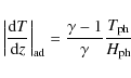
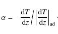
For a convectively unstable layer
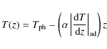
For the atmosphere above the convectively unstable layer, the temperature distribution is:
![\begin{displaymath}T(z) = T_{\rm ph} + (T_{\rm cor}-T_{\rm pho})\left(\frac{1}{2...
...nh\left(\frac{z-z_{\rm tr}}{w_{\rm tr}}+1\right)\right]\right)
\end{displaymath}](/articles/aa/full_html/2009/48/aa12455-09/img46.png)
|
(10) |
where we consider
For the initial magnetic field we consider a horizontal and uniform
magnetic field distribution, located within the upper levels of the
unstable layer below the photosphere. Initially, the magnetic flux
sheet is oriented along the positive x-direction.
Thus, the magnetic field strength is:
where

where
Similar to the 2D experiments by Isobe et al. (2007), we take the plasma beta at the flux sheet (
Using Eqs. (6), (12) and (13), we can derive the distributions of density, the gas pressure and the magnetic field
strength in the flux sheet by solving the equation of magnetostatic balance:
|
(14) |
Initially, a small velocity perturbation is imposed on the magnetic flux sheet, to excite the convective Parker-instability. The component of the velocity perturbation along the flux sheet has the form:
where we take a small amplitude, A=0.05 and a wavelength,
For the computational domain, we assume periodic boundary conditions for the x and y directions. At the lower boundary at
![]() the boundary is symmetric (rigid conducting wall). At the top boundary (
the boundary is symmetric (rigid conducting wall). At the top boundary (
![]() )
the z derivatives of all variables are set to zero.
We also include a wave damping zone for z>65 where fluctuations of velocity, gas pressure and density decay exponentially with time.
)
the z derivatives of all variables are set to zero.
We also include a wave damping zone for z>65 where fluctuations of velocity, gas pressure and density decay exponentially with time.
The physical size of the numerical box is
![]() ,
,
![]() and
and
![]() .
The number of the grid points are
Nx=400, Ny=140 and Nz=200. The grid spacing is uniform in the horizontal directions,
.
The number of the grid points are
Nx=400, Ny=140 and Nz=200. The grid spacing is uniform in the horizontal directions,
![]() and
and
![]() .
In the z direction
.
In the z direction
![]() for
for ![]() ,
while it increases for larger heights.
,
while it increases for larger heights.
![\begin{figure}
\par\includegraphics[width=7.5cm,clip]{12455f2a.eps}\includegraph...
...clip]{12455f2c.eps}\includegraphics[width=7.5cm,clip]{12455f2d.eps}
\end{figure}](/articles/aa/full_html/2009/48/aa12455-09/img74.png)
|
Figure 2: The distribution of vz at the photosphere for t=20, 30, 40 and 50 ( from up-left to bottom-right). The horizontal planes extend across the whole numerical domain in the x- and y-direction. |
| Open with DEXTER | |
![\begin{figure}
\mbox{\includegraphics[width=5.8cm,clip]{12455f3a.eps}\hspace*{4m...
...}\hspace*{4mm}
\includegraphics[width=5.8cm,clip]{12455f3f.eps} }
\end{figure}](/articles/aa/full_html/2009/48/aa12455-09/img76.png)
|
Figure 3:
Left: distribution of Bz at z=1 for t=50, t=60 and t=70. The horizontal velocity distribution is shown with the
overplotted arrows.
Right: the same, for the distribution of
|
| Open with DEXTER | |
3 Emergence into the photosphere
3.1 Rising magnetic field and velocity pattern.
Due to the initial velocity perturbation and the convectively unstable layer below the photosphere, a number of magnetic loops are formed out of the initial magnetic flux sheet. The magnetic field develops a number of undulations and adopts an overall serpentine-like shape. Initially, the perturbed segments (loop-like structures) of the magnetic flux sheet rise due to the Parker instability. The size of the undulations and the draining of the plasma along the fieldlines at the crests of the rising loops are characteristic of the Parker instability. As the instability develops, the plasma slides down along the magnetic field, enhancing the magnetic buoyancy of the rising loops.
The instability in the sheet is excited by the initial velocity perturbation.
The characteristic wavelength in the magnetic field that appears during the dynamical evolution of the system is between
![]() and
and
![]() .
Notice that
the Parker instability in an isothermal gas has its maximum growth rate for a wavelength in the range
.
Notice that
the Parker instability in an isothermal gas has its maximum growth rate for a wavelength in the range
![]() .
Now, the evolution of the
convective-Parker instability is determined by modes with large wavelength, independent of the initial perturbation wavelength.
The perturbation with the most unstable wavelength is efficiently created by nonlinear mode coupling (Nozawa et al. 1992).
Modes with small wavelength are stabilized due to the
downward magnetic tension of the fieldlines.
.
Now, the evolution of the
convective-Parker instability is determined by modes with large wavelength, independent of the initial perturbation wavelength.
The perturbation with the most unstable wavelength is efficiently created by nonlinear mode coupling (Nozawa et al. 1992).
Modes with small wavelength are stabilized due to the
downward magnetic tension of the fieldlines.
Figure 2 shows the evolution of vz at z=1 for t=20,
30, 40 and 50. As time goes on, the velocity field loses its initial
random configuration and consists of a network of cells that have
upflows in their middle section. At the boundaries between the cells,
there are pronounced downflows. At
![]() ,
the size of the cells varies from
,
the size of the cells varies from
![]() to
to
![]() .
This network of upflows and downflows forms a pattern, which evolves
dynamically in space and is highly time-dependent. The deformation of
the initial velocity field is due to the emergence of the
sub-photospheric magnetic field. The upflows correspond to the upward
rising motion of the magnetic field and the downflows occur at the
periphery of the emerging loop-like structures as the plasma drains
down along the fieldlines of the loops.
.
This network of upflows and downflows forms a pattern, which evolves
dynamically in space and is highly time-dependent. The deformation of
the initial velocity field is due to the emergence of the
sub-photospheric magnetic field. The upflows correspond to the upward
rising motion of the magnetic field and the downflows occur at the
periphery of the emerging loop-like structures as the plasma drains
down along the fieldlines of the loops.
The initial appearance of the magnetic loops is shown by the the magnetic fieldlines, which are overplotted in the four panels of Fig. 2. The fieldlines have been traced from random points at the base of the photosphere. At t=20, they are almost straight and they are oriented along the x-axis. Eventually (t=30 and t=40), some segments are rising forming loop-like structures that eventually emerge through the photosphere. There is a good comparison between the location of the upflow regions and the sites of rising loops. Also the downflows appear in between the rising loops and become stronger as the loops rise higher into the atmosphere (t=50). Also, notice that now the magnetic fieldlines are not oriented only along the x-axis but they can follow various directions in the three-dimensional volume. This is due to various reasons: one is the shearing that some fieldlines experience due to the initial velocity perturbation, a second reason is the appearance of interchange modes due to the strong non-linear coupling of the magnetic field. At later times, due to the three-dimensional expansion of the field, neighbouring fieldlines may reconnect and change their connectivity. The initial evolution of the magnetic field distribution at the photosphere is discussed in more detail in the next section.
3.2 Distribution of magnetic field and plasma  .
.
![\begin{figure}
\par\includegraphics[width=8.8cm,clip]{12455f4a.eps}\par\includeg...
...{12455f4c.eps}\par\includegraphics[width=8.8cm,clip]{12455f4d.eps}
\end{figure}](/articles/aa/full_html/2009/48/aa12455-09/img82.png)
|
Figure 4: Evolution of the magnetic field strength for t=60,70,90 and t=130. The vertical slice shows the distribution of the total magnetic field strength at y=71. The horizontal slice shows the Bz distribution at the base of the photosphere. The range of values for Bz is -2 to 2. The horizontal and vertical planes extend across the whole numerical domain, in the x-y and x-z directions respectively. |
| Open with DEXTER | |
The evolution of the magnetic field distribution shows, that although the network of mixed polarities appears to be complex, there is an order on the appearance of the flux sources. Positive polarities appear at the left side of the rising loops and move leftward while negative polarities appear on the right side of the emerging fields and move towards the right side of the numerical domain. The apparent order on the initial flux distribution is mainly due to the fact that the original flux sheet is uniform and orientated along the x-direction.
Overplotted is the horizontal velocity field (arrows) onto the horizontal plane. The velocity distribution shows that a) there is a general diverging flow as the two opposite polarities stream away from the central region of the emerging loops and b) there are converging motions at the internetwork, at the boundaries between the emerging loops. This is due to the expansion of the rising magnetic field and the downflows from the crest to the periphery of the three-dimensional loops.
The apparent horizontal motion of the migrating polarities may reach speeds of about 1-2 km s-1. As they drift apart, flux sources may experience encounters with opposite-polarity fields. These flux cancellation events are common, especially during the advanced stage (t > 70) of the evolution of the system, leading to a general decrease of the total unsigned flux at the photosphere.
![\begin{figure}
\par\includegraphics[width=7.7cm,clip]{12455f5a.eps}\par\vspace*{2mm}
\includegraphics[width=7.7cm,clip]{12455f5b.eps}
\end{figure}](/articles/aa/full_html/2009/48/aa12455-09/img83.png)
|
Figure 5: Top: height-time profile of a loop that is emerging into the corona. Bottom: distribution of gas pressure (dashed line) and magnetic pressure (solid line) along height (within the emerging loop), at t=80. |
| Open with DEXTER | |
In the right column of Fig. 3, the
![]() is shown for the same height (z=1) and times.
We find that at t=50,
the rising magnetic field has just crossed the isothermal photosphere.
The magnetic loops experience horizontal expansion but they cannot
proceed with further emergence into the outer atmosphere. After
is shown for the same height (z=1) and times.
We find that at t=50,
the rising magnetic field has just crossed the isothermal photosphere.
The magnetic loops experience horizontal expansion but they cannot
proceed with further emergence into the outer atmosphere. After
![]() plasma
plasma ![]() is reduced, as more field rises from the interior
to the photosphere, and obtains values smaller than one in
various regions across the photosphere. The build-up of the magnetic pressure
at these regions is associated with the increase of Bz and the emergence of more magnetic flux from the solar interior as we discussed
above.
is reduced, as more field rises from the interior
to the photosphere, and obtains values smaller than one in
various regions across the photosphere. The build-up of the magnetic pressure
at these regions is associated with the increase of Bz and the emergence of more magnetic flux from the solar interior as we discussed
above.
As the plasma ![]() ,
the magnetic pressure exceeds the gas pressure and the first flux elements begin to rise and
expand above the photosphere. Similar to the work by Archontis et al. (2004), we find that as plasma
,
the magnetic pressure exceeds the gas pressure and the first flux elements begin to rise and
expand above the photosphere. Similar to the work by Archontis et al. (2004), we find that as plasma ![]() ,
the evolution occurs on the basis of the magnetic buoyancy instability
experience by the plasma above the photosphere. More precisely, we find
that the strong stabilizing term
,
the evolution occurs on the basis of the magnetic buoyancy instability
experience by the plasma above the photosphere. More precisely, we find
that the strong stabilizing term
![]() (
(![]() being the superadiabaticity of the atmosphere) adopts small values and actually becomes smaller than
being the superadiabaticity of the atmosphere) adopts small values and actually becomes smaller than
![]() .
The latter term describes the instability-promoting effect of the decrease of the magnetic field
with height in the upper part of the rising magnetic field.
.
The latter term describes the instability-promoting effect of the decrease of the magnetic field
with height in the upper part of the rising magnetic field.
By t=70, stronger field has reached the photosphere and, thus, plasma ![]() is reduced significantly. The distribution at the photosphere shows
a sporadic decrease of plasma
is reduced significantly. The distribution at the photosphere shows
a sporadic decrease of plasma ![]() :
at this stage of the evolution the magnetic flux sheet does not emerge
as a whole structure but it rather consists of individual magnetic
loops that rise due to their own magnetic pressure force. The emergence
of the magnetic loops into the corona is discussed in the next section.
:
at this stage of the evolution the magnetic flux sheet does not emerge
as a whole structure but it rather consists of individual magnetic
loops that rise due to their own magnetic pressure force. The emergence
of the magnetic loops into the corona is discussed in the next section.
4 Emergence into the corona
4.1 Local evolution of the magnetic field
To study the emergence of the undulating magnetic field into the
corona we follow first of all the rising motion of one magnetic loop,
which is part of the large-scale magnetic flux system. We focus our
attention on regions at the photosphere where plasma ![]() is small and, thus, magnetic pressure is large. One of the regions is
located at 60<x<80 and 45<y<60 (see middle-left panel in Fig. 3). The magnetic field meets the photosphere in this region and
eventually forms an
is small and, thus, magnetic pressure is large. One of the regions is
located at 60<x<80 and 45<y<60 (see middle-left panel in Fig. 3). The magnetic field meets the photosphere in this region and
eventually forms an ![]() -loop shape that rises into the corona. Figure 5 (top panel) shows the temporal evolution of the height
of the apex of this loop. More precisely, we plot the
height of the apex at x=65 and y=52. The magnetic field strength
is weak at the top of the rising loops and, thus, we define the apex as the point where the magnitude of B is
-loop shape that rises into the corona. Figure 5 (top panel) shows the temporal evolution of the height
of the apex of this loop. More precisely, we plot the
height of the apex at x=65 and y=52. The magnetic field strength
is weak at the top of the rising loops and, thus, we define the apex as the point where the magnitude of B is ![]() 10-4.
A side-view visualization of this loop together with its rising motion through the atmosphere is shown in the next section.
10-4.
A side-view visualization of this loop together with its rising motion through the atmosphere is shown in the next section.
The emergence starts when the magnetic field experiences the upward
forcing of the initial velocity perturbation. The apex of the magnetic
loop reaches the photosphere at
![]() .
The further upward motion involves lifting up dense plasma against
gravity, within the photosphere that is stable against the convective
instability. Thus, the loop continues to rise through the photosphere
but with small velocity and considerable expansion in the transverse
direction (see also bottom panels in Fig. 3). After t=50, plasma
.
The further upward motion involves lifting up dense plasma against
gravity, within the photosphere that is stable against the convective
instability. Thus, the loop continues to rise through the photosphere
but with small velocity and considerable expansion in the transverse
direction (see also bottom panels in Fig. 3). After t=50, plasma ![]() drops sufficiently so that the evolution of the magnetic field
occurs due to the buoyancy instability
as has been described in Archontis et al. (2004) and Murray et al. (2006). Now the magnetic field is emerging all the way up into the corona and experiences a runaway
expansion.
drops sufficiently so that the evolution of the magnetic field
occurs due to the buoyancy instability
as has been described in Archontis et al. (2004) and Murray et al. (2006). Now the magnetic field is emerging all the way up into the corona and experiences a runaway
expansion.
Figure 5 (bottom panel) shows the distribution of the magnetic and the gas pressure along height, within the emerging loop. At t=80, the apex of the loop has reached a height just above z=20 and, thus, it is well inside corona. Notice that the magnetic pressure (solid line) is larger than the gas pressure (dashed line) inside the rising, magnetized volume of the field and, thus, the plasma is free to expand as it rises into the higher atmosphere.
4.2 Global evolution of the magnetic field.
We now study the global evolution and rise of the magnetic field into the corona. Figure 4 consists of four panels that show the
emergence of the magnetic field at four different times. The coloured contours on the transparent vertical slice (y=52) show
the magnitude of the magnetic field strength
![]() .
The horizontal slice shows the vertical component of the magnetic field, Bz, just above the base of the photosphere (z=1). The fieldlines are
traced from the vertical slice, at points within the emerging field.
.
The horizontal slice shows the vertical component of the magnetic field, Bz, just above the base of the photosphere (z=1). The fieldlines are
traced from the vertical slice, at points within the emerging field.
At t=60 (top panel in Fig. 4), the initial magnetic flux sheet has developed a number of loops (L1 to L4), which are inter-connected with serpentine-like fieldlines (u1 and u2). From the distribution of Bz at photospheric heights, we find that the dips of the fieldlines are located at regions between the positive and negative polarities of neighbouring loops. Some of the dips cross the photosphere and have their lowest concave part below the photosphere, while other dips are tangent to the photosphere at BPs. Most of the loops have entered the chromosphere/transition region but they have not yet expanded dynamically into the corona. Examples of emerging loops are loops L2 and L3, at the center of the vertical slice. The evolution of the central-right loop (L3) was studied in the previous section. Notice, that on the two sides of the loops L2 and L3 there are segments of fieldlines that do not form discrete, coherent loops, which rise dynamically into the atmosphere. These fieldlines undergo loose undulations at low photospheric heights (see u1 and u2). This is the typical topology of the magnetic field at this stage of the evolution: a network of emerging loops and low-lying undulating fieldlines, which are joined across the photosphere.
At t=70, the visualization of
![]() at the vertical slice shows the formation of four main magnetic loops across the x-direction.
The two central loops continue to rise into the atmosphere. They also
expand sideways as they rise. Due to the expansion, neighbouring
fieldlines approach to each other and reconnect. Reconnection occurs
between fieldlines with opposite directions that come into contact at
the vicinity of the dips. Due to successive reconnection at various
heights, longer loops without pronounced undulations may form during
the dynamical evolution of the system. One example of this process is
the formation of the two loops (L3 and L4) at the right side of the
computational volume. Reconnection occured between these loops and the
undulating fieldlines (u2) in the spare region between the loops at
earlier times (e.g. after t=60). As a result, longer loops have been formed, which in turn, they will come closer together and reconnect
at later times. This is similar to the process of resistive flux emergence, which has been presented in theoretical grounds by Pariat et al. (2004) and
in numerical experiments by Isobe et al. (2007).
at the vertical slice shows the formation of four main magnetic loops across the x-direction.
The two central loops continue to rise into the atmosphere. They also
expand sideways as they rise. Due to the expansion, neighbouring
fieldlines approach to each other and reconnect. Reconnection occurs
between fieldlines with opposite directions that come into contact at
the vicinity of the dips. Due to successive reconnection at various
heights, longer loops without pronounced undulations may form during
the dynamical evolution of the system. One example of this process is
the formation of the two loops (L3 and L4) at the right side of the
computational volume. Reconnection occured between these loops and the
undulating fieldlines (u2) in the spare region between the loops at
earlier times (e.g. after t=60). As a result, longer loops have been formed, which in turn, they will come closer together and reconnect
at later times. This is similar to the process of resistive flux emergence, which has been presented in theoretical grounds by Pariat et al. (2004) and
in numerical experiments by Isobe et al. (2007).
Indeed, at t=90 there are reconnected fieldlines that join the crests of the two loops L3 and L4 (seen at t=70) forming a new, longer flux system L3 (with a typical loop-like shape and a length of about 9-10 Mm), which has emerged well into the corona. Also, some of the low-lying fieldlines that appear at the central part of the domain at t=70 and t=90, start from the positive polarity of the far-left magnetic loop (L1) and they end up in the crest of the right loop (L4). Actually, these fieldlines join all the loops without going through BPs. These are also reconnected fieldlines for which all of their segments start to rise above the photosphere and, eventually, into the outer atmosphere.
At t=130, most of the magnetic fieldlines that previously enveloped the emerging loops have now been reconnected at and above photospheric heights, forming two long magnetic flux systems (L1 and L2) that reach heights around z=65. At this specific time and position along the y-direction, there is only one discernible U-shaped dip at the center of the domain where the fieldlines touch the low atmosphere. Later on, this U-dip will be diminished when local reconnection events will join the two lateral magnetic systems.
It is worthwhile mentioning that the fieldlines that belong to the two flux systems (L1 and L2) have different shapes at different heights. Fieldlines, which are lying at low heights underneath the large expanding outer loops, still possess undulations along their lengths. This topology is an indication of reconnection that occurs at different heights during the process of flux emergence. With this mechanism, the large reconnected fieldlines get detached from the low atmosphere and are free to rise into the corona. The evolution of the magnetic field described in this section is typical of the global magnetic field in this numerical experiment.
![\begin{figure}
\par\includegraphics[width=8.2cm,clip]{12455f6a.eps}\par\includegraphics[width=8.2cm,clip]{12455f6b.eps}
\end{figure}](/articles/aa/full_html/2009/48/aa12455-09/img92.png)
|
Figure 6: Top: close-up in one of the dips that magnetic fieldlines (white lines) possess along the undulating magnetic flux system at t=50. The arrows show the direction of the full velocity vector. Bottom: the same location but at a later stage of the evolution of the system (t=60). The color of the arrows is changing from dark blue (negative values, downflows) to red (positive values, upflows). |
| Open with DEXTER | |
5 Resistive emergence and Ellerman bombs
One question that arises from the resistive flux emergence model is the role of reconnection on the emergence of the magnetic flux system into the higher atmosphere. Our simulation show that reconnection occurs firstly at the photosphere when the sufficiently long flux sheet becomes subject to the Parker instability, developing a series of undulations.
Figure 6 is a closeup of the magnetic reconnection at the low atmosphere. The size of the part of the domain shown in this figure is
![]() ,
y=30 and
,
y=30 and
![]() .
The horizontal black line shows the base of the photosphere. The arrows
show the direction of the full velocity vector and the white lines are
the magnetic field lines, which are traced from the flanks of the two
magnetic loops into contact. The two loops shown in this figure are a
small part of the whole undulating magnetic field. At t=50
(top panel), there are converging downflows at the flanks of the loops
due to the rising motion of the magnetic field. The magnetic fieldlines
form a U-dip at the interface. In fact, these dips are sites where
dense plasma is trapped as it is drained down by the flows, along the
flanks of the emerging field. Since the temperature gradient in the
sub-photospheric layer is superadiabatic, the concave part of the
magnetic flux system sinks rapidly and, thus, induces converging flows
towards the interface and enhances the downflows along the interface.
When the oppositely directed fieldlines of the magnetic loops come
close together, a current layer builds up at their interface. There is
an average number of twelve grid points across the current layers,
which are formed in the computational volume during the evolution of
the system. Reconnection starts to occur at the current layer,
producing bidirectional flows (t=60, bottom panel).
In this regime, the flow is upward at the photosphere with a value of
.
The horizontal black line shows the base of the photosphere. The arrows
show the direction of the full velocity vector and the white lines are
the magnetic field lines, which are traced from the flanks of the two
magnetic loops into contact. The two loops shown in this figure are a
small part of the whole undulating magnetic field. At t=50
(top panel), there are converging downflows at the flanks of the loops
due to the rising motion of the magnetic field. The magnetic fieldlines
form a U-dip at the interface. In fact, these dips are sites where
dense plasma is trapped as it is drained down by the flows, along the
flanks of the emerging field. Since the temperature gradient in the
sub-photospheric layer is superadiabatic, the concave part of the
magnetic flux system sinks rapidly and, thus, induces converging flows
towards the interface and enhances the downflows along the interface.
When the oppositely directed fieldlines of the magnetic loops come
close together, a current layer builds up at their interface. There is
an average number of twelve grid points across the current layers,
which are formed in the computational volume during the evolution of
the system. Reconnection starts to occur at the current layer,
producing bidirectional flows (t=60, bottom panel).
In this regime, the flow is upward at the photosphere with a value of ![]() 1 km s-1. There is also a downflow, which is moving mainly within the sub-photospheric
layer, with smaller velocity of about 0.2 km s-1.
1 km s-1. There is also a downflow, which is moving mainly within the sub-photospheric
layer, with smaller velocity of about 0.2 km s-1.
Reconnection also changes the magnetic topology around the reconnection site. The dense plasma that is trapped in the U-dips stays below the photosphere in new reconnecting fieldlines, which are twisted and all together adopt the shape of small flux tubes. Higher up, the fieldlines that were previously linked to the photosphere, have now been reconnected and are rising into the higher atmosphere. The new reconnected fieldlines can envelope the two loops from above, and thus, connect the two far ends of the loops. This is a typical example of how reconnection works between neighbouring magnetic loops at this stage of the evolution of the system. By this process the magnetic field is getting rid of the dense plasma and gradually it rises through successive atmospheric heights.
![\begin{figure}
\par\includegraphics[width=7.5cm,clip]{12455f7a.eps}\par\vspace*{...
...}\includegraphics[width=6.8cm,clip]{12455f7b.eps}\hspace*{3.5mm} }\end{figure}](/articles/aa/full_html/2009/48/aa12455-09/img95.png)
|
Figure 7: Top: distribution of the total current density. Bottom: distribution of temperature. Both are taken at z=6 (low chromosphere) and for t=90. |
| Open with DEXTER | |
As we discussed in the previous section, reconnection occurs at various
heights of the atmosphere due to the three-dimensional emergence of the
magnetic loops and to the non-linear and highly dynamic evolution of
the system. Figure 7 shows the distribution of the current
density (
![]() )
and the temperature at the low chromosphere (z=6) at t=90.
There are many current layers, which are formed at the interface
between flux sources with opposite polarities. The flux sources belong
to different loops that emerge and approach to each other. In some of
these sites the current density is especially strong. For example,
three sites with pronounced currents are the regions around x=75, y=50, x=32, y=48
and x=55, y=65.
From the temperature distribution, we find that there is a good
correlation between sites with strong current density and enhanced
temperature. Notice, that the cool
regions correspond to the plasma that expands adiabatically as the loops emerge.
)
and the temperature at the low chromosphere (z=6) at t=90.
There are many current layers, which are formed at the interface
between flux sources with opposite polarities. The flux sources belong
to different loops that emerge and approach to each other. In some of
these sites the current density is especially strong. For example,
three sites with pronounced currents are the regions around x=75, y=50, x=32, y=48
and x=55, y=65.
From the temperature distribution, we find that there is a good
correlation between sites with strong current density and enhanced
temperature. Notice, that the cool
regions correspond to the plasma that expands adiabatically as the loops emerge.
![\begin{figure}
\par\hspace*{-4mm}\includegraphics[width=7.8cm,clip]{12455f8a.eps...
...2mm}
\hspace*{-4mm}\includegraphics[width=7.5cm,clip]{12455f8c.eps}
\end{figure}](/articles/aa/full_html/2009/48/aa12455-09/img97.png)
|
Figure 8: Top: bi-directional flow that is heated due to reconnection at the low chromosphere. Middle: distribution of temperature and density along the x-direction at the low chromosphere for y=65 and t=90. Bottom: distribution of entropy along the x-direction at the low chromosphere for y=65 and t=70 (blue), t=80 (red) and t=90 (black). |
| Open with DEXTER | |
The enhanced temperature is due to effective reconnection that occurs
at the sites with strong current layers. As a result of reconnection,
bi-directional flows are produced at the chromosphere. Figure 8 shows the reconnection outflow, which is produced at t=90 in the region around
x=55 and y=65. The change in the direction of the
outflows occurs at
![]() .
Thus, at this stage of the evolution, the reconnection site is at the low chromosphere. The upflow is emitted within
the chromosphere and the downflow towards the photosphere. According to our units,
the upward velocity of the bi-directional flow in the chromosphere/transition region could be as high as
.
Thus, at this stage of the evolution, the reconnection site is at the low chromosphere. The upflow is emitted within
the chromosphere and the downflow towards the photosphere. According to our units,
the upward velocity of the bi-directional flow in the chromosphere/transition region could be as high as
![]() km s-1 and the downflow
could reach values up to
km s-1 and the downflow
could reach values up to
![]() km s-1. It is worth mentioning that
in a few cases the upward outflows may reach velocities up to 20 km s-1, as the hot plasma is ejected above the reconnection site. These high speed outflows may
account for surge-like features.
km s-1. It is worth mentioning that
in a few cases the upward outflows may reach velocities up to 20 km s-1, as the hot plasma is ejected above the reconnection site. These high speed outflows may
account for surge-like features.
We are now looking at some of the properties of the magnetized plasma
that is emitted due to reconnection that occurs in various locations
within the rising magnetic flux system. Such locations are shown in
Fig. 7 (marked with rectangular boxes).
The horizontal profiles (along the x-direction) of temperature and density at z=6, y=65 and t=90 are shown in Fig. 8.
The distribution shows that
the temperature is enhanced in three regions by a factor of 1.3,
relative to the temperature of the initial background atmosphere at
this height. The density distribution shows a good correlation with the
temperature. Density takes large values at
![]() ,
,
![]() and
and
![]() .
The maximum value shows that the density increases by a factor of 2.7,
relative to the density of the background plasma.
The values of the relative enhancement of the temperature and density
of the plasma may vary at different sites of reconnection. As an
example, the density enhancement could reach a factor of 4 at this
height during the evolution of the system and the increase of
temperature may vary between a factor of 1.1 and 1.5.
.
The maximum value shows that the density increases by a factor of 2.7,
relative to the density of the background plasma.
The values of the relative enhancement of the temperature and density
of the plasma may vary at different sites of reconnection. As an
example, the density enhancement could reach a factor of 4 at this
height during the evolution of the system and the increase of
temperature may vary between a factor of 1.1 and 1.5.
It is worthwhile mentioning that temperature and density enhancments could also be produced by adiabatic compression and vertical bi-directional flows can be formed via pressure increase when there are horizontal converging flows. This could be another mechanism (alternative to magnetic reconnection) responsible for the formation of small scale brightenings at various atmospheric heights (e.g. EBs). However, to show that this is not true in all cases in our numerical experiment, we calculate the time evolution (at three different times) of entropy across three possible sites of EBs (bottom panel in Fig. 8). Adiabatic compression is an isentropic process and, thus, entropy should not increase at the locations of density and temperature enhancment. However, entropy shows a pronounced increase at these locations while it remains aprroximately invariant in between them. Current density, temperature and plasma density have also local maxima at the same sites (see middle panel in Fig. 8). We should mention that we have also calculated the parallel electric field and we found that it has a maximum at the EBs. Although, we use a small explicit resistivity, the parallel electric field in narrow layers (the current sheets) can reach values that are a few hundred times larger than the average value of the background plasma. This means that resistive effects, such as magnetic reconnection, are very important at the locations of EBs.
![\begin{figure}
\par\includegraphics[width=7.8cm,clip]{12455f9a.eps}\par\vspace*{2mm}
\includegraphics[width=7.8cm,clip]{12455f9b.eps}
\end{figure}](/articles/aa/full_html/2009/48/aa12455-09/img104.png)
|
Figure 9: Top: time evolution of various energies. Bottom: variation of current density along time. |
| Open with DEXTER | |
Figure 9 shows the time variation of various energies (top panel) and the current density (bottom panel) around the site of a
possible EB (located at
![]() ,
,
![]() and starting around t=80). The magnetic, thermal and kinetic energies are defined by
and starting around t=80). The magnetic, thermal and kinetic energies are defined by
|
(15) |
|
(16) |
![\begin{displaymath}E_{\rm kin} = \int \int \int \frac{1}{2} \rho \left[u{x}^2 + u_{y}^2 + u_{z}^2\right] {\rm d}x {\rm d}y {\rm d}z
\end{displaymath}](/articles/aa/full_html/2009/48/aa12455-09/img109.png)
|
(17) |
respectively. They are integrated in the region: 48<x<56, 60<y<67 and 3<z<9. It should be noted that for the thermal energy we calculate
This result, together with the sudden change of connectivity of the fieldlines and the existense of bidirectional flows, strongly suggests that magnetic reconnection is the most plausible driving mechanism for these EBs that are formed in our experiment.
Based on the physical extent (along the x- and y-directions) to which the temperature and density show a significant relative increase, one can
estimate an average size for the afore-mentioned bright structures.
From Fig. 7 this rough estimate gives a typical width (x-size) between 4 and 5 (![]() 720-900 km)
and a typical length between 4 and 6 (
720-900 km)
and a typical length between 4 and 6 (![]() 720-1080 km). The shape of these
structures is mainly determined by the geometry of the magnetic fields
that come into contact and produce them via reconnection. At sites
where segments of three or more rising loops interact (e.g., x=30, y=48 in Fig. 7),
they look like bright sources with a roundish shape. This is the most
common shape that they adopt during the evolution of the system.
However, there are other places where the interfaces between
interacting magnetic fields are more stretched (e.g., 67<x<78, 50<x<68)
with an elongated shape, like bright lanes. The small-scale brightenings have an average life-time of
720-1080 km). The shape of these
structures is mainly determined by the geometry of the magnetic fields
that come into contact and produce them via reconnection. At sites
where segments of three or more rising loops interact (e.g., x=30, y=48 in Fig. 7),
they look like bright sources with a roundish shape. This is the most
common shape that they adopt during the evolution of the system.
However, there are other places where the interfaces between
interacting magnetic fields are more stretched (e.g., 67<x<78, 50<x<68)
with an elongated shape, like bright lanes. The small-scale brightenings have an average life-time of
![]() (i.e. 6-7 min).
In few cases, these features (e.g., at x=20, y=30) may exist for
(i.e. 6-7 min).
In few cases, these features (e.g., at x=20, y=30) may exist for
![]() (i.e.
(i.e. ![]() 11 min).
11 min).
5.1 Comparison with observations: Ellerman bombs
The above characteristics of the small-scale bright features compare well with quantitative measurements of EBs.
Kurokawa et al. (1982) found that EBs have a typical length of ![]() 1 arcsec and are associated with photospheric downflows.
Matsumoto et al. (2008) reported downflows at the photosphere (
1 arcsec and are associated with photospheric downflows.
Matsumoto et al. (2008) reported downflows at the photosphere (![]() 0.2 km s-1) and upflows in the chromosphere (
0.2 km s-1) and upflows in the chromosphere (![]() 1-3 km s-1).
Dara et al. (1997) also reported strong upflows in the chromosphere. Georgoulis et al. (2002) investigated the statistical properties of EBs in an
emerging flux region and found that EBs were correlated with downflows (
1-3 km s-1).
Dara et al. (1997) also reported strong upflows in the chromosphere. Georgoulis et al. (2002) investigated the statistical properties of EBs in an
emerging flux region and found that EBs were correlated with downflows (![]() 0.5 km s-1) at the photosphere. Also, non-LTE analysis of
spectral profiles of EBs showed strong downflows (
0.5 km s-1) at the photosphere. Also, non-LTE analysis of
spectral profiles of EBs showed strong downflows (![]() 10 km s-1) between the upper photosphere and
the low chromosphere (Socas-Navarro et al. 2006).
An interesting result was reported by Matsumoto et al. (2008) who performed spectroscopic observations of EBs in an active region in order to investigate
the height dependence of gas flows in EBs. They found that
bidirectional flows may start between the lower photosphere and the lower chromosphere. The above results are in agreement with
our simulations, where bidirectional flows are produced (see Figs. 6 and 8) at various heights between photosphere and chromosphere.
10 km s-1) between the upper photosphere and
the low chromosphere (Socas-Navarro et al. 2006).
An interesting result was reported by Matsumoto et al. (2008) who performed spectroscopic observations of EBs in an active region in order to investigate
the height dependence of gas flows in EBs. They found that
bidirectional flows may start between the lower photosphere and the lower chromosphere. The above results are in agreement with
our simulations, where bidirectional flows are produced (see Figs. 6 and 8) at various heights between photosphere and chromosphere.
Rust et al. (1977) found that some EBs are related to H![]() surges, which are commonly thought to be the result of magnetic reconnection
at the low chromosphere. Kurokawa et al. (1982) and Kitai (1983) also detected strong upflows (
surges, which are commonly thought to be the result of magnetic reconnection
at the low chromosphere. Kurokawa et al. (1982) and Kitai (1983) also detected strong upflows (![]() 8 km s-1), which may account for small surges,
at the location of Ebs. These observations are also consistent with the high-velocity upflows produced in our simulations, above
the locations of EBs during the evolution of the system. At the region
of EBs, Socas Navvaro (2005a) found strong currents, which indicates
that EBs may be associated with reconnection. Figure 7 shows that regions with enhanced current density are favourable sites for the appearance of EBs
in our numerical experiments.
8 km s-1), which may account for small surges,
at the location of Ebs. These observations are also consistent with the high-velocity upflows produced in our simulations, above
the locations of EBs during the evolution of the system. At the region
of EBs, Socas Navvaro (2005a) found strong currents, which indicates
that EBs may be associated with reconnection. Figure 7 shows that regions with enhanced current density are favourable sites for the appearance of EBs
in our numerical experiments.
Kitai (1983) found that a density enhancement (by a factor of 5) and a hot temperature gradient (![]() 1500 K) may account for the line broadening in EBs.
Georgoulis et al. (2002) and Pariat et al. (2004) also found that the temperature increases by
1500 K) may account for the line broadening in EBs.
Georgoulis et al. (2002) and Pariat et al. (2004) also found that the temperature increases by ![]() 2000 K at the sites of EBs.
In our simulations, the density enhancement is close to the value reported by Kitai (1983).
The increase of temperature is larger, possibly due to the fact that
the energy equation in our numerical experiments does not include all
the thermodynamical terms (such as thermo-conduction) and the equation
of state is for an ideal gas. Thermal and non-thermal semi-empirical
atmospheric models for EBs have been presented by Fang et al. (2006) and Chen et al. (2001). They found that the temperature enhancement in the lower chromosphere is about
600-1300 K.
The increase of temperature was reduced
by 100-300 K when the nonthermal effects were included in the model.
2000 K at the sites of EBs.
In our simulations, the density enhancement is close to the value reported by Kitai (1983).
The increase of temperature is larger, possibly due to the fact that
the energy equation in our numerical experiments does not include all
the thermodynamical terms (such as thermo-conduction) and the equation
of state is for an ideal gas. Thermal and non-thermal semi-empirical
atmospheric models for EBs have been presented by Fang et al. (2006) and Chen et al. (2001). They found that the temperature enhancement in the lower chromosphere is about
600-1300 K.
The increase of temperature was reduced
by 100-300 K when the nonthermal effects were included in the model.
Finally, many observations have shown that the typical lifetime of EBs is 10-20 min (Nindos & Zirin 1998; Kurokawa et al. 1982; Qiu et al. 2000). Pariat studied the UV time profiles of EBs and found that the distribution of lifetimes for individual impulses (associated with the EBs) peaks between 3 and 4 min. In our simulations, the lifetime of the EBs is between 6 and 11 min.
![\begin{figure}
\par\includegraphics[width=8.5cm,clip]{12455f10.eps}
\end{figure}](/articles/aa/full_html/2009/48/aa12455-09/img116.png)
|
Figure 10: 3D topology of magnetic fieldlines as the undulating magnetic flux system emerges through the atmosphere (t=90). The temperature distribution at the low chromosphere (z=6) is shown by the horizontal slice. The latter extends across the whole numerical domain, in the x- and y-directions. |
| Open with DEXTER | |
![\begin{figure}
\mbox{\includegraphics[width=5.8cm,clip]{1245511a.eps}\hspace*{4m...
...}\hspace*{4mm}
\includegraphics[width=5.8cm,clip]{1245511f.eps} }
\end{figure}](/articles/aa/full_html/2009/48/aa12455-09/img117.png)
|
Figure 11:
Left: distribution of Bz at the photosphere for t=70, t=80 and t=90 ( from top to bottom). The projection of the
horizontal velocity field vector on the slice is shown by the arrows. Right: distribution of
|
| Open with DEXTER | |
5.2 Topology around Ellerman bombs
Figure 10 shows a number of fieldlines that have been traced from the EBs, at the low chromosphere at t=90. The horizontal slice shows the distribution of temperature with the same scaling as that in Fig. 7. The 3D visualization of the topology of the field reveals that the majority of the EBs are found in locations where the magnetic fieldlines have a V-shape. Note, that a substantial number of fieldlines possess more than one V-like dips along their length and, thus, many EBs appear to be inter-connected with the same fieldlines. As we have shown in Sect. 3.2, effective reconnection, which occurs at the locations of EBs, is essential for the emergence of the magnetic flux system into the higher atmosphere. The general topology of the magnetic field in association with the location of the EBs is reminiscent of the model proposed by Pariat et al. (2004) who reported that the dips of undulatory flux tubes are cospatial with EBs.
Another interesting topological feature in Fig. 10 is the dramatic change of connectivity of fieldlines around some of the sites of EBs. For example, notice the sudden change in the connectivity of the blue and white fieldlines that they pass through the EBs in the locations marked with rectangular boxes. The long overplotted (black) arrows show the direction of the full magnetic field vector along individual sets of fieldlines. It is likely that in such complex topologies, quasi-seperatrix layers (QSLs) are formed at the interfaces between neighbouring magnetic systems that interact during the emergence of the field. The concept of current sheet formation and reconnection in QSLs has been studied extensively in the past (Démoulin 2006; Aulanier et al. 2005; Priest & Démoulin 1995). Therefore, it is expected that QSLs may occur in the low atmosphere and EBs are triggered somewhere along QSLs. EB triggering by magnetic reconnection on QSLs was also favoured by the observational data obtained by Georgoulis et al. (2002).
6 Late evolution of the magnetic field
In this section we study the late evolution (![]() )
of the magnetic field at the photosphere. At the beginning, the
magnetic field is emerging at the photosphere in the form of horizontal
field with an average field strength of about 600 G. The
horizontal field is stronger than the vertical magnetic field. Until,
)
of the magnetic field at the photosphere. At the beginning, the
magnetic field is emerging at the photosphere in the form of horizontal
field with an average field strength of about 600 G. The
horizontal field is stronger than the vertical magnetic field. Until,
![]() ,
the horizontal field constitutes almost
,
the horizontal field constitutes almost ![]() of the total magnetic field strength, in most of the photospheric layer at z=1.
The magnetic field continues to emerge and start to rise into the outer
atmosphere, in the form of magnetic loops. As the emerging loops rise,
the magnetic field is moving from the initial site of emergence towards
the flanks of the emerging loops and, thus, it adopts a more pronounced
vertical configuration. At t=70, the
horizontal magnetic field is still more space-filling than the vertical magnetic field. However, the strongest field (e.g., field with values larger than
of the total magnetic field strength, in most of the photospheric layer at z=1.
The magnetic field continues to emerge and start to rise into the outer
atmosphere, in the form of magnetic loops. As the emerging loops rise,
the magnetic field is moving from the initial site of emergence towards
the flanks of the emerging loops and, thus, it adopts a more pronounced
vertical configuration. At t=70, the
horizontal magnetic field is still more space-filling than the vertical magnetic field. However, the strongest field (e.g., field with values larger than ![]() of the maximum value of
of the maximum value of
![]() )
is nearly all vertical. After t=70, the average values of the vertical and the horizontal magnetic field at
the photosphere do not change dramatically.
)
is nearly all vertical. After t=70, the average values of the vertical and the horizontal magnetic field at
the photosphere do not change dramatically.
6.1 Intensification of the magnetic field
Although the estimate of the average magnetic field does not go under
significant changes, there are still regions at the photosphere where,
after t=70,
![]() and Bz increase locally.
The topology of the flows plays a role in the local increase of the
field. In the following, we will present examples of flux
concentrations, that undergo intensification during the late evolution
of the system.
and Bz increase locally.
The topology of the flows plays a role in the local increase of the
field. In the following, we will present examples of flux
concentrations, that undergo intensification during the late evolution
of the system.
Figure 11 (left column) shows the time evolution of Bz
at the photosphere. The horizontal velocity field is overplotted
(arrows) on the photospheric plane. The magnetic field is emerging at
various places and then it expands in the atmosphere. The expansion of
the field drives horizontal outflows away from each emerging region.
The overal topology of the velocity field shows that the horizontal
outflows are converging at the boundaries between neighbouring emerging
regions. Also, due to the ![]() -like shape
of the emerging loops, there is drainage of mass (and, thus, downflows) along the edges of the loops.
-like shape
of the emerging loops, there is drainage of mass (and, thus, downflows) along the edges of the loops.
![\begin{figure}
\par\includegraphics[width=7.5cm,clip]{1245512a.eps}\par\vspace*{...
...2mm}
\hspace{1.5mm}\includegraphics[width=7.3cm,clip]{1245512c.eps}
\end{figure}](/articles/aa/full_html/2009/48/aa12455-09/img121.png)
|
Figure 12:
Top: distribution of Bz along the y-direction at x=77 and z=1. Times are: t=60 (green), t=70 (red), t=75 (blue) and t=80 (black).
Middle: distribution of vz in the same region for t=70 (red), t=75 (blue) and t=80. Bottom: intensification of
|
| Open with DEXTER | |
The site between x=75-80 and y=55-60 is located between three emerging loops. The dominant polarity of the magnetic field in this region
is negative. Figure 11 (top panel) shows the enhancement of Bz: at t=60 the negative flux concentration has field strength around 3 (![]() 900 Gauss) and
at t=80 (6-7 min later) the magnetic field has strength as high as 7 (
900 Gauss) and
at t=80 (6-7 min later) the magnetic field has strength as high as 7 (![]() 2 kG). The middle panel in Fig. 12 shows the distribution
of Vz in this region.
The magnetic field is enhanced where strong downflows exist. The speed of the donflows increases from 0.5 to
2 kG). The middle panel in Fig. 12 shows the distribution
of Vz in this region.
The magnetic field is enhanced where strong downflows exist. The speed of the donflows increases from 0.5 to ![]() 0.8 (4.5 to 7 km s-1)
between t=70 and t=80.
The acceleration of the downflows is due to the dense plasma that is
drained through the footpoints of the loops and the superadiabaticity
of the atmosphere. Also, the converging flows, which are caused due to
the expansion of nearby emerging fields are
0.8 (4.5 to 7 km s-1)
between t=70 and t=80.
The acceleration of the downflows is due to the dense plasma that is
drained through the footpoints of the loops and the superadiabaticity
of the atmosphere. Also, the converging flows, which are caused due to
the expansion of nearby emerging fields are ![]() 2 km s-1 and
2 km s-1 and ![]() 5 km s-1 along the x- and y-direction respectively.
5 km s-1 along the x- and y-direction respectively.
Due to the strong downflows and the effective drainage of mass, the
plasma becomes partially evacuated in the upper layers (e.g, the
density is less at z=1 than at z=-1). Also, the density in this region is less by a factor of ![]() 0.8 than the average density of the background atmosphere.
The relative decrease in the gas pressure is a factor of
0.8 than the average density of the background atmosphere.
The relative decrease in the gas pressure is a factor of ![]() 0.7.
Thus, the converging outflows from the expanding loops are able to
compress the fluid and strengthen the magnetic field. Intensification
stops when pressure balance is achieved between the magnetic flux
concentration and the external atmosphere.
0.7.
Thus, the converging outflows from the expanding loops are able to
compress the fluid and strengthen the magnetic field. Intensification
stops when pressure balance is achieved between the magnetic flux
concentration and the external atmosphere.
The horizontal magnetic field can be intensified by a similar mechanism. Figure 11
(right column) shows that the field is horizontal mainly at the
boundaries between emerging magnetic loops. The cross section of two
loops that emerge to the photosphere at different locations are those
close to x=15, y=55 and x=22, y=30 respectively (top-right panel in Fig. 11).
As time goes on, the magnetic field expands and the edges of the rising
loops come into contact (bottom-right panel). This is when the
horizontal segments of the magnetic field, which belong to the
interacting emerging loops, are folded constructively since they have
almost parallel orientation. Again, the fluid at the interface is
compressed by the converging motions and the strength of the field
increases accordingly. The bottom panel in Fig. 12 shows the distribution of the horizontal magnetic field
along the y-direction at x=18.7 for three different times. The two local maxima correspond to the horizontal segments of the two emerging loops.
At this stage of the evolution,
![]() is close to 3.2 (between
900-1000 G).
Eventually, they approach to each other and collide, increasing the magnitude of the horizontal field to
is close to 3.2 (between
900-1000 G).
Eventually, they approach to each other and collide, increasing the magnitude of the horizontal field to ![]() 5.3 (1590 G).
5.3 (1590 G).
6.2 New emergence of flux
A possible consequence of the convectively unstable layer below the
photosphere is the emergence of new magnetic flux, driven by convective
upflows. An episode of emergence of new magnetic flux is shown in
Fig. 11. At t=70 the uppermost layers of the emerging field
have reached the photosphere (
x=45, y=42). As the magnetic field continues to rise, it
expands laterally and modifies the preexisting flow pattern at the
photosphere. The upward rising motion appears as an upflow cell that
eventually induces diverging (down)flows at the periphery of the
emerging field. The area of the emerging field, when it rises initially
at the photosphere, is ![]()
![]() .
.
![\begin{figure}
\par\includegraphics[width=7.8cm,clip]{1245513a.eps}\par\vspace*{2mm}
\hspace*{4mm}\includegraphics[width=8.4cm,clip]{1245513b.eps}
\end{figure}](/articles/aa/full_html/2009/48/aa12455-09/img123.png)
|
Figure 13: Top: the distribution of the total magnetic field strength along height as it is calculated at the central part of the new flux emerging region. The distribution is shown for t=70 (black), t=80 (red) and t=90 (blue). Bottom: distribution of temperature (black line) and current density (red) along the x-axis, at z=20 and t=90. |
| Open with DEXTER | |
The emergence of the magnetic field into the higher atmosphere is shown in Fig. 13 (top panel). We plot the distribution of the total magnetic field strength along height at the center of the cross section of the emerging field for t=70, 80 and 90. The field strength, when it firstly crosses the photospheric layer, can be as high as 450 G. Eventually, as it expands, the field strength drops (under the condition of magnetic flux conservation) to 320 G at t=90. By that time, a considerable amount of emerging field has been advanced into the higher levels of the atmosphere.
The rise of the new emerging field into the corona does not proceed uninhibited. The earlier dynamical rise and expansion of neighbouring magnetic loops has formed a pre-existing ambient field in the corona. The interaction between the new emerging field and the pre-existing magnetized atmosphere produces rotational discontinuities, which might lead to the development of layers with enhanced current density. The appearance of bright structures in the corona could be the result of the local enhancement in the temperature of these layers.
The bottom panel in Fig. 13
shows the increase of temperature in the corona when a current layer is
formed at the interface between the emerging flux and ambient field.
The ambient field is formed by the expansion of magnetized plasma that
belongs to a neighbouring flux system. The local maximum of the current
density (red line) at
![]() correlates well with the enhancement of the temperature, which could be
a factor of 2.8 higher than the initial coronal temperature (
correlates well with the enhancement of the temperature, which could be
a factor of 2.8 higher than the initial coronal temperature (![]() 1 MK).
1 MK).
In our numerical experiments, rotational discontinuities in the higher atmosphere are formed not only when new magnetic flux interacts with ambient field but also due to the very dynamical interaction between neighbouring emerging loops. The fieldlines of the expanding loops are free to move in three dimensional space and, thus, it is not unlikely that sets of fieldlines with opposite orientations press against each other and form strong current sheets. An example of this type of interaction between emerging fields is given in Fig. 4. The region between the loops L3 and L4 (marked with an arrow, at t=70 and t=90) is where current density increases, followed by an enhancement of the temperature in the corona. The 3D interaction between an emerging twisted flux tube (or flux sheet) and a pre-existing field in the corona has been studied in more detail by Archontis & Hood (2008), Galsgaard et al. (2005) and Isobe et al. (2005).
7 Summary and discussion
Through our numerical experiments we have investigate the emergence of a magnetic flux system with undulations in three dimensions. Magnetic fields with a sea-serpent configuration appear in various places in the solar surface e.g., in the central part of an emerging active region. We show that the emergence into the corona occurs through reconnection events at successive atmospheric heights, from the photosphere up to the outer solar atmosphere. This resistive emergence process leads to the formation of large-scale magnetic flux systems, with sizes of a few tens of Mm, which rise into the corona. The magnetic field is free to emerge and expand, since the dense plasma, which accumulates at the dips between undulations, is off-loaded in the low atmosphere by reconnection.
By-products of the efficient reconnection process are small-scale brightenings, which appear at various atmospheric heights. In the upper photosphere/chromosphere, these events can account for Ellerman bombs. Our numerical results show a good comparison with some of the major characteristics of EBs as recorded by observations. However, for a direct comparison with observational data, extra thermodynamical aspects need to be included in the numerical models, since the heat loss/gain due to radiative cooling and heat conduction are important. Also, the inclusion of partial ionization could play a role in the formation of current sheets and the temperature enhancement at the sites of EBs. In the upper atmosphere, brightenings appear due to the dynamical interaction between newly emerging flux and pre-existing coronal field or between emerging fieldlines that come into contact and form strong current layers.
One difference with the corresponding 2D numerical study (Isobe et al. 2007) is the development of interchange modes for the magnetic field and the excitation of non-linear, dynamic coupling between emerging fields. This leads to the formation of a complex network of rising loops that emerge into the atmosphere over a range of temporal and spatial scales. Moreover, a series of interesting phenomena are produced such as: the formation of many structures with enhanced current density and a series of bright features throughout the atmosphere, the existence of bi-directional flows that in few cases may reach high velocities, flux cancellation at the low atmosphere and so on.
The appearance of magnetic field undulations in our experiments is due to the Parker instability, which is triggered by the initial velocity perturbation on the uniform magnetic flux sheet. The convectively unstable layer supports the formation of the undulations, which eventually grow forming magnetic loop-like structures that emerge through the photosphere. However, in our experiments the sub-photospheric layer is not a realistic convective envelope. Other 3D MHD radiative simulations, that include a convection zone (Cheung et al. 2008), identify convective dynamics as the main reason for the formation of serpentine-like fieldlines at the photosphere. More observations and numerical studies are required for a detailed study of this issue. On the other hand, we assertain that the further rise of the magnetic field into the higher atmosphere is independent of the cause for the appearance of undulations at the photosphere.
The general evolution of the magnetic field in our model is similar to those in the resistive emergence model proposed by Pariat et al. (2004). Although there is a good comparison between our numerical results, the theoretical model by Pariat et al. (2004) and relevant observations, more experiments are required to study the effect of varying the parameters used in our simulations such as, the field strength, thickness and location of the flux sheet, the superadiabaticity and the inclusion of extra heating/cooling sources in the energy equation.
AcknowledgementsWe gratefully acknoweledge the financial support of STFC and the European Commission through the SOLAIRE Network (MTRN-CT-2006-035484). The simulations were performed on the STFC and SRIF funded UKMHD cluster, at the University of St Andrews.
References
- Archontis, V., & Hood, A. W. 2008, ApJ, 674, L113 [NASA ADS] [CrossRef]
- Archontis, V., Moreno-Insertis, F., Galsgaard, K., Hood, A., & O'Shea, E. 2004, A&A, 426, 1047 [NASA ADS] [EDP Sciences] [CrossRef]
- Aulanier, G., Pariat, E., & Démoulin, P. 2005, A&A, 444, 961 [NASA ADS] [EDP Sciences] [CrossRef]
- Bernasconi, P. N., Rust, D. M., Georgoulis, M. K., & Labonte, B. J. 2002, Sol. Phys., 209, 119 [NASA ADS] [CrossRef]
- Chen, P.-F., Fang, C., & Ding, M.-D. D. 2001, Chinese J. Astron. Astrophys., 1, 176 [NASA ADS] [CrossRef]
- Cheung, M. C. M., Schüssler, M., Tarbell, T. D., & Title, A. M. 2008, ApJ, 687, 1373 [NASA ADS] [CrossRef]
- Dara, H. C., Alissandrakis, C. E., Zachariadis, T. G., & Georgakilas, A. A. 1997, A&A, 322, 653 [NASA ADS]
- Démoulin, P. 2006, Adv. Space Res., 37, 1269 [NASA ADS] [CrossRef]
- Ding, M. D., Henoux, J.-C., & Fang, C. 1998, A&A, 332, 761 [NASA ADS]
- Ellerman, F. 1917, ApJ, 46, 298 [NASA ADS] [CrossRef]
- Fang, C., Tang, Y. H., Xu, Z., Ding, M. D., & Chen, P. F. 2006, ApJ, 643, 1325 [NASA ADS] [CrossRef]
- Galsgaard, K., Moreno-Insertis, F., Archontis, V., & Hood, A. 2005, ApJ, 618, L153 [NASA ADS] [CrossRef]
- Georgoulis, M. K., Rust, D. M., Bernasconi, P. N., & Schmieder, B. 2002, ApJ, 575, 506 [NASA ADS] [CrossRef]
- Harvey, K., & Harvey, J. 1973, Sol. Phys., 28, 61 [NASA ADS] [CrossRef]
- Isobe, H., Miyagoshi, T., Shibata, K., & Yokoyama, T. 2005, Nature, 434, 478 [NASA ADS] [CrossRef]
- Isobe, H., Miyagoshi, T., Shibata, K., & Yokoyama, T. 2006, PASJ, 58, 423 [NASA ADS]
- Isobe, H., Tripathi, D., & Archontis, V. 2007, ApJ, 657, L53 [NASA ADS] [CrossRef]
- Kitai, R. 1983, Sol. Phys., 87, 135 [NASA ADS] [CrossRef]
- Kurokawa, H., Kawaguchi, I., Funakoshi, Y., & Nakai, Y. 1982, Sol. Phys., 79, 77 [NASA ADS] [CrossRef]
- Mackay, D. H., Longbottom, A. W., & Priest, E. R. 1999, Sol. Phys., 185, 87 [NASA ADS] [CrossRef]
- Mandrini, C. H., Démoulin, P., Schmieder, B., Deng, Y. Y., & Rudawy, P. 2002, A&A, 391, 317 [NASA ADS] [EDP Sciences] [CrossRef]
- Matsumoto, T., Kitai, R., Shibata, K., et al. 2008, PASJ, 60, 95 [NASA ADS]
- Murray, M. J., Hood, A. W., Moreno-Insertis, F., Galsgaard, K., & Archontis, V. 2006, A&A, 460, 909 [NASA ADS] [EDP Sciences] [CrossRef]
- Nindos, A., & Zirin, H. 1998, Sol. Phys., 182, 381 [NASA ADS] [CrossRef]
- Nozawa, S., Shibata, K., Matsumoto, R., et al. 1992, ApJS, 78, 267 [NASA ADS] [CrossRef]
- Pariat, E., Aulanier, G., Schmieder, B., et al. 2004, ApJ, 614, 1099 [NASA ADS] [CrossRef]
- Pariat, E., Schmieder, B., Berlicki, A., et al. 2007, A&A, 473, 279 [NASA ADS] [EDP Sciences] [CrossRef]
- Parker, E. N. 1966, ApJ, 145, 811 [NASA ADS] [CrossRef]
- Priest, E. R., & Démoulin, P. 1995, J. Geophys. Res., 100, 23443 [NASA ADS] [CrossRef]
- Qiu, J., Ding, M. D., Wang, H., Denker, C., & Goode, P. R. 2000, ApJ, 544, L157 [NASA ADS] [CrossRef]
- Rust, D. M., Webb, D. F., & MacCombie, W. 1977, Sol. Phys., 54, 53 [NASA ADS] [CrossRef]
- Seehafer, N. 1986, Sol. Phys., 105, 223 [NASA ADS] [CrossRef]
- Shibata, K., Tajima, T., Matsumoto, R., et al. 1989, ApJ, 338, 471 [NASA ADS] [CrossRef]
- Socas-Navarro, H., Martínez Pillet, V., Elmore, D., et al. 2006, Sol. Phys., 235, 75 [NASA ADS] [CrossRef]
- Spruit, H. C., Title, A. M., & van Ballegooijen, A. A. 1987, Sol. Phys., 110, 115 [NASA ADS] [CrossRef]
- Titov, V. S., & Démoulin, P. 1999, A&A, 351, 707 [NASA ADS]
- Watanabe, H., Kitai, R., Okamoto, K., et al. 2008, ApJ, 684, 736 [NASA ADS] [CrossRef]
- Zwaan, C. 1985, Sol. Phys., 100, 397 [NASA ADS] [CrossRef]
All Figures
|
|
Figure 1: Left: the initial stratification of the background atmosphere (t=0). Right: the coloured contours show the initial distribution of the vertical component of velocity at the xy plane at z=-5. The horizontal slice extends across the whole numerical domain in the x- and y-direction. |
| Open with DEXTER | |
| In the text | |
|
|
Figure 2: The distribution of vz at the photosphere for t=20, 30, 40 and 50 ( from up-left to bottom-right). The horizontal planes extend across the whole numerical domain in the x- and y-direction. |
| Open with DEXTER | |
| In the text | |
|
|
Figure 3:
Left: distribution of Bz at z=1 for t=50, t=60 and t=70. The horizontal velocity distribution is shown with the
overplotted arrows.
Right: the same, for the distribution of
|
| Open with DEXTER | |
| In the text | |
|
|
Figure 4: Evolution of the magnetic field strength for t=60,70,90 and t=130. The vertical slice shows the distribution of the total magnetic field strength at y=71. The horizontal slice shows the Bz distribution at the base of the photosphere. The range of values for Bz is -2 to 2. The horizontal and vertical planes extend across the whole numerical domain, in the x-y and x-z directions respectively. |
| Open with DEXTER | |
| In the text | |
|
|
Figure 5: Top: height-time profile of a loop that is emerging into the corona. Bottom: distribution of gas pressure (dashed line) and magnetic pressure (solid line) along height (within the emerging loop), at t=80. |
| Open with DEXTER | |
| In the text | |
|
|
Figure 6: Top: close-up in one of the dips that magnetic fieldlines (white lines) possess along the undulating magnetic flux system at t=50. The arrows show the direction of the full velocity vector. Bottom: the same location but at a later stage of the evolution of the system (t=60). The color of the arrows is changing from dark blue (negative values, downflows) to red (positive values, upflows). |
| Open with DEXTER | |
| In the text | |
|
|
Figure 7: Top: distribution of the total current density. Bottom: distribution of temperature. Both are taken at z=6 (low chromosphere) and for t=90. |
| Open with DEXTER | |
| In the text | |
|
|
Figure 8: Top: bi-directional flow that is heated due to reconnection at the low chromosphere. Middle: distribution of temperature and density along the x-direction at the low chromosphere for y=65 and t=90. Bottom: distribution of entropy along the x-direction at the low chromosphere for y=65 and t=70 (blue), t=80 (red) and t=90 (black). |
| Open with DEXTER | |
| In the text | |
|
|
Figure 9: Top: time evolution of various energies. Bottom: variation of current density along time. |
| Open with DEXTER | |
| In the text | |
|
|
Figure 10: 3D topology of magnetic fieldlines as the undulating magnetic flux system emerges through the atmosphere (t=90). The temperature distribution at the low chromosphere (z=6) is shown by the horizontal slice. The latter extends across the whole numerical domain, in the x- and y-directions. |
| Open with DEXTER | |
| In the text | |
|
|
Figure 11:
Left: distribution of Bz at the photosphere for t=70, t=80 and t=90 ( from top to bottom). The projection of the
horizontal velocity field vector on the slice is shown by the arrows. Right: distribution of
|
| Open with DEXTER | |
| In the text | |
|
|
Figure 12:
Top: distribution of Bz along the y-direction at x=77 and z=1. Times are: t=60 (green), t=70 (red), t=75 (blue) and t=80 (black).
Middle: distribution of vz in the same region for t=70 (red), t=75 (blue) and t=80. Bottom: intensification of
|
| Open with DEXTER | |
| In the text | |
|
|
Figure 13: Top: the distribution of the total magnetic field strength along height as it is calculated at the central part of the new flux emerging region. The distribution is shown for t=70 (black), t=80 (red) and t=90 (blue). Bottom: distribution of temperature (black line) and current density (red) along the x-axis, at z=20 and t=90. |
| Open with DEXTER | |
| In the text | |
Copyright ESO 2009
Current usage metrics show cumulative count of Article Views (full-text article views including HTML views, PDF and ePub downloads, according to the available data) and Abstracts Views on Vision4Press platform.
Data correspond to usage on the plateform after 2015. The current usage metrics is available 48-96 hours after online publication and is updated daily on week days.
Initial download of the metrics may take a while.