| Issue |
A&A
Volume 508, Number 3, December IV 2009
|
|
|---|---|---|
| Page(s) | 1443 - 1452 | |
| Section | The Sun | |
| DOI | https://doi.org/10.1051/0004-6361/200911876 | |
| Published online | 01 October 2009 | |
A&A 508, 1443-1452 (2009)
Hard X-ray emission from a flare-related jet
H. M. Bain - L. Fletcher
Department of Physics and Astronomy, University of Glasgow, Glasgow, G12 8QQ, UK
Received 17 Febuary 2009 / Accepted 24 September 2009
Abstract
Aims. We aim to understand the physical conditions in a jet
event which occurred on the 22nd of August 2002, paying particular
attention to evidence for non-thermal electrons in the jet material.
Methods. We investigate the flare impulsive phase using
multiwavelength observations from the Transition Region and Coronal
Explorer (TRACE) and the Reuven Ramaty High Energy Spectroscopic Imager
(RHESSI) satellite missions, and the ground-based Nobeyama
Radioheliograph (NoRH) and Radio Polarimeters (NoRP).
Results. We report what we believe to be the first observation
of hard X-ray emission formed in a coronal jet. We present radio
observations which confirm the presence of non-thermal electrons
present in the jet at this time. The evolution of the event is best
compared with the magnetic reconnection jet model in which emerging
magnetic field interacts with the pre-existing coronal field. We
calculate an apparent jet velocity of ![]() 500
500
![]() which is consistent with model predictions for jet material accelerated by the
which is consistent with model predictions for jet material accelerated by the
![]() force resulting in a jet velocity of the order of the Alfvén speed (
force resulting in a jet velocity of the order of the Alfvén speed (![]() 100-1000
100-1000
![]() ).
).
Key words: Sun: activity - Sun: flares - Sun: X-rays, gamma rays - Sun: radio radiation
1 Introduction
Solar X-ray jets (transient bursts of collimated flows of plasma) were first observed by the Yohkoh Solar X-ray Telescope (SXT: Tsuneta et al. 1991) (Shibata et al. 1992; Strong et al. 1992).
It has been shown that jets are spatially correlated with active
regions, X-ray bright points and regions of emerging flux and can be
associated with small footpoint flares (Shibata et al. 1992,1994). Several studies of X-ray jets (Shimojo et al. 1996; Canfield et al. 1996) yielded characteristic properties such as length and width observed to be in the range of a few 104-105 km and
![]() -105 km respectively. Apparent jet velocities of 10-1000 km s-1 (average
-105 km respectively. Apparent jet velocities of 10-1000 km s-1 (average ![]()
![]() )
are observed and the kinetic energy of the jet is thought to be 1025-1028 erg. Shimojo & Shibata (2000) analysed a number of jets and their footpoint flares finding values for jet temperature and density of 3-8 MK
(average 5.6 MK) and 0.7-
)
are observed and the kinetic energy of the jet is thought to be 1025-1028 erg. Shimojo & Shibata (2000) analysed a number of jets and their footpoint flares finding values for jet temperature and density of 3-8 MK
(average 5.6 MK) and 0.7-
![]() (average
(average
![]() )
respectively. More recently observations of solar X-ray jets have been made using data from the Hinode X-ray Telescope (XRT: Golub et al. 2007) (Savcheva et al. 2007; Chifor et al. 2008; Shimojo et al. 2007).
The results are generally consistent with the previous studies however
XRT's improved spatial and temporal resolution has revealed many
smaller X-ray jet events.
)
respectively. More recently observations of solar X-ray jets have been made using data from the Hinode X-ray Telescope (XRT: Golub et al. 2007) (Savcheva et al. 2007; Chifor et al. 2008; Shimojo et al. 2007).
The results are generally consistent with the previous studies however
XRT's improved spatial and temporal resolution has revealed many
smaller X-ray jet events.
It has been observed that in general there are two kinds of
jet; 1) the anemone-shaped jet, consistent with emerging photospheric
field interacting with pre-existing coronal field which is vertical or
oblique; 2) the two-sided-loop type where the interaction occurs with
overlying horizontal coronal magnetic field (Shimojo et al. 1996).
Observational properties such as the jet velocity are an important
diagnostic of the jet acceleration mechanism. Several jet models have
been suggested, most models at some stage invoke magnetic reconnection
as the source of a rapid injection of energy. The magnetic reconnection
jet model (Shimojo et al. 1996; Heyvaerts et al. 1977; Shimojo & Shibata 2000)
describes a bundle of emerging photospheric field reconnecting with a
pre-existing overlying coronal magnetic field. As the result of the
reconnection, surrounding plasma is heated to X-ray emitting
temperatures and subsequently ejected out along the direction of the
reconnected field. Plasma propagating downwards forms X-ray emitting
loops at the foot of the jet. Observations have shown that H
![]() surges are often associated with X-ray jets (Canfield et al. 1996).
In the reconnection model this is as a result of a ``magnetic
sling-shot'' effect caused by magnetic tension as the previously highly
stressed emerging field straightens out. This results in the ejection
of cool plasma (10 000 K) that had been supported by the
field. Magnetohydrodynamic simulations of this scenario describe the
observations well (Moreno-Insertis et al. 2008; Yokoyama & Shibata 1995; Nishizuka et al. 2008). Ejected jet material accelerated by the
surges are often associated with X-ray jets (Canfield et al. 1996).
In the reconnection model this is as a result of a ``magnetic
sling-shot'' effect caused by magnetic tension as the previously highly
stressed emerging field straightens out. This results in the ejection
of cool plasma (10 000 K) that had been supported by the
field. Magnetohydrodynamic simulations of this scenario describe the
observations well (Moreno-Insertis et al. 2008; Yokoyama & Shibata 1995; Nishizuka et al. 2008). Ejected jet material accelerated by the
![]() force will have a velocity of the order of the Alfvén speed.
force will have a velocity of the order of the Alfvén speed.
There have been observations of jets with a helical twisted shape. The
``magnetic twist'' model explains this as the result of reconnection
between twisted and untwisted magnetic field (Shibata et al. 1992; Alexander & Fletcher 1999; Pariat et al. 2009; Shibata & Uchida 1986). The ejected material is accelerated by the
![]() force as the twisted magnetic field relaxes. As with the magnetic
reconnection model, the ejected material will have a velocity of the
order of the Alfvén speed. Magnetic islands of cool plasma form within
the twisted field, described by the ``melon-seed'' model for spicules (Uchida 1969), which propagate out as the field relaxes. This also occurs at the Alfvén speed.
force as the twisted magnetic field relaxes. As with the magnetic
reconnection model, the ejected material will have a velocity of the
order of the Alfvén speed. Magnetic islands of cool plasma form within
the twisted field, described by the ``melon-seed'' model for spicules (Uchida 1969), which propagate out as the field relaxes. This also occurs at the Alfvén speed.
Other models suggest that the acceleration mechanism is related to gas pressure. Evaporation flows occur as the result of a rapid release of energy in the corona. In this situation the jet velocity will be of the order of the sound speed (Shibata et al. 1992; Sterling et al. 1993)
Type III radio bursts, caused by unstable beams of accelerated electrons, are often associated with jets. Electrons accelerated in association with jets have been detected in space (Christe et al. 2008). Another diagnostic of fast electrons is bremsstrahlung X-ray emission which can be observed with the Reuven Ramaty High Energy Spectroscopic Imager, (RHESSI: Lin et al. 2002). However until now no evidence of hard X-ray emission has been observed directly from the jet in the corona. This could be because it is rare to find a coronal jet dense enough to provide a bremsstrahlung target for the electrons, or hot enough to generate high energy thermal emission. In this paper we report what we believe to be the first observation of hard X-ray emission formed in a coronal jet. We observe a flare-related jet which occurred on the 22nd August 2002. Observations from the Transition Region Coronal Explorer, (TRACE: Handy et al. 1999) and RHESSI satellite missions are presented. The event was also observed by the ground-based Nobeyama Radioheliograph (NoRH: Nakajima et al. 1994) and Polarimeters (NoRP: Torii et al. 1979). Together these observations cover the X-ray, extreme ultraviolet (EUV) and radio regimes.
2 Event overview
![\begin{figure}
\par\includegraphics[width=8.7cm]{11876f1.ps}
\end{figure}](/articles/aa/full_html/2009/48/aa11876-09/img13.png)
|
Figure 1: From top to bottom: GOES, RHESSI, TRACE and NoRH lightcurves. Vertical dashed lines represent 32 s time intervals used for RHESSI imaging (see Fig. 5). (See electronic version for colour plots.) |
| Open with DEXTER | |
![\begin{figure}
\par\includegraphics[scale=0.4]{11876f2.ps}
\end{figure}](/articles/aa/full_html/2009/48/aa11876-09/img14.png)
|
Figure 2:
TRACE 195Å images for selected times throughout the event showing
the evolution of the jet. These images have a time resolution of |
| Open with DEXTER | |
The jet occurred on the 22nd of August 2002 preceding a GOES M5.4 class
flare. Time profiles from GOES, RHESSI, TRACE and NoRH can be seen in
Fig. 1. Vertical dashed lines represent 32 s time intervals used for RHESSI imaging (see Fig. 5
later). At 01:40 GOES, RHESSI and NoRH 17 GHz show an increase in
the signal above background levels. This is due to a small source
slightly north of the jet region, centred at (825
![]() ,
-225
,
-225
![]() )
which does not appear to be related to the jet. The evolution of the
event can be followed best using high resolution TRACE observations
(see Fig. 2), only available for the 195 Å passband during the event. These images have a time resolution of
)
which does not appear to be related to the jet. The evolution of the
event can be followed best using high resolution TRACE observations
(see Fig. 2), only available for the 195 Å passband during the event. These images have a time resolution of ![]() 9 s and a spatial resolution of 1
9 s and a spatial resolution of 1
![]() .
Dark black areas show regions of saturation. This is particularly
noticeable later in the event when the hot loops form. The high
contrast is to allow faint features to be visible. Under normal active
region conditions this wavelength is dominated by Fe XII line emission at
.
Dark black areas show regions of saturation. This is particularly
noticeable later in the event when the hot loops form. The high
contrast is to allow faint features to be visible. Under normal active
region conditions this wavelength is dominated by Fe XII line emission at
![]() 6 K. During flares it will be dominated by higher temperature plasma, providing both Fe XXIV and Ca XVII line emissions (5
6 K. During flares it will be dominated by higher temperature plasma, providing both Fe XXIV and Ca XVII line emissions (5 ![]() 106 K and (1-2)
106 K and (1-2) ![]() 107 K)
and a significant thermal continuum due to free-free and free-bound
emission, which is in fact dominant at temperatures of around
107 K)
and a significant thermal continuum due to free-free and free-bound
emission, which is in fact dominant at temperatures of around
![]() (Feldman et al. 1999).
The images were exposure normalised using the Solarsoft routine
trace_prep. Cosmic ray spikes were also removed using this routine.
(Feldman et al. 1999).
The images were exposure normalised using the Solarsoft routine
trace_prep. Cosmic ray spikes were also removed using this routine.
Preflare activity can be seen in the region as early as ![]() 01:25 (Fig. 2a). From
01:25 (Fig. 2a). From ![]() 01:27 a complex system of twisted loops begin to brighten (Figs. 2b-2f)
and appears to rise. At 01:35 part of this system becomes twisted
in a configuration similar to that found in models of the kink
instability (Török & Kliem 2005). This can be seen best a few minutes later when it is at its brightest in Fig. 2e
(see arrow). Although faint, this feature is present right up until the
main ejection. To the north-west, at the right foot of the twisted
field (820
01:27 a complex system of twisted loops begin to brighten (Figs. 2b-2f)
and appears to rise. At 01:35 part of this system becomes twisted
in a configuration similar to that found in models of the kink
instability (Török & Kliem 2005). This can be seen best a few minutes later when it is at its brightest in Fig. 2e
(see arrow). Although faint, this feature is present right up until the
main ejection. To the north-west, at the right foot of the twisted
field (820
![]() ,
-270
,
-270
![]() ),
faint material starts to move outward, starting at 01:31, along a
separate large scale loop or possibly even open interplanetary field.
This is seen at its brightest in Fig. 2d (see
arrow). Small amounts of faint material continues to move in this
direction for several minutes before the main ejection, becoming more
obvious at 01:42 (see Figs. 2e and 2f).
Unfortunately a gap in the TRACE data between 01:45:49 and 01:49:44
prevents us following this material with TRACE. For the purpose of
understanding this complex event, we label pre-jet activity, including
the ejection missed by TRACE up to 01:49:44, as ``pre-gap''.
),
faint material starts to move outward, starting at 01:31, along a
separate large scale loop or possibly even open interplanetary field.
This is seen at its brightest in Fig. 2d (see
arrow). Small amounts of faint material continues to move in this
direction for several minutes before the main ejection, becoming more
obvious at 01:42 (see Figs. 2e and 2f).
Unfortunately a gap in the TRACE data between 01:45:49 and 01:49:44
prevents us following this material with TRACE. For the purpose of
understanding this complex event, we label pre-jet activity, including
the ejection missed by TRACE up to 01:49:44, as ``pre-gap''.
During the data gap increased amounts of material are ejected.
This can be seen, in images immediately after the data gap, as plasma
at greater heights in the corona (Figs. 2g and 2h). Also from the images immediately after the data gap (Figs. 2g and 2h)
we can see that the rising twisted loops appear to have opened to the
right of the kink feature, which is still visible (see arrow in
Fig. 2h). This results in a large amount of plasma being ejected, beginning at ![]() 01:50:35.
The feature to the left of the jet can then be seen to straighten out.
The ejected material appears to untwist slightly as the twist from the
emerging field is transferred to the ``open'' field lines of the jet as
a result of reconnection. The material then passes out of the TRACE
field of view after
01:50:35.
The feature to the left of the jet can then be seen to straighten out.
The ejected material appears to untwist slightly as the twist from the
emerging field is transferred to the ``open'' field lines of the jet as
a result of reconnection. The material then passes out of the TRACE
field of view after ![]() 01:52.
01:52.
Material continues to be ejected until ![]() 02:09 (Figs. 2g-2m).
The total duration of jetting material is therefore around 40 min.
Hot loops can be seen forming between EUV ribbons, roughly (820
02:09 (Figs. 2g-2m).
The total duration of jetting material is therefore around 40 min.
Hot loops can be seen forming between EUV ribbons, roughly (820
![]() ,
-260
,
-260
![]() ), as early as
), as early as ![]() 01:51:30. These loops brighten, expand and then fade away over the course of an hour
(Figs. 2n-2p).
Activity from 01:49:44 onwards, including the main ejection, is
labelled ``post-gap''. In this paper we concentrate on the impulsive
and rise phase of the event i.e. post-gap times when the main ejection
of material occurs.
01:51:30. These loops brighten, expand and then fade away over the course of an hour
(Figs. 2n-2p).
Activity from 01:49:44 onwards, including the main ejection, is
labelled ``post-gap''. In this paper we concentrate on the impulsive
and rise phase of the event i.e. post-gap times when the main ejection
of material occurs.
![\begin{figure}
\par\includegraphics[width=8.7cm]{11876f3.ps}
\end{figure}](/articles/aa/full_html/2009/48/aa11876-09/img18.png)
|
Figure 3: Velocity timeslice showing jet intensity as a function of height and time. Vertical dash-dot line shows the time at which the jet emission passes out of the TRACE field of view. Dashed lines on insert image show the region used for the analysis. Asterisks and solid line shows a fit to the faint front edge of the jet at the 5% level. Diamonds and dashed line shows a fit to points determined from tracking a brightly emitting source of plasma by eye. |
| Open with DEXTER | |
Due to the jet extending beyond the TRACE field of view we were unable
to determine its full length. However an estimate of jet width was
found to be
![]() km. This was determined by eye and assigned an error of
km. This was determined by eye and assigned an error of ![]() 5 pixels.
To calculate the apparent velocity of the jet during the main ejection
a timeslice image was created using post-gap images (Fig. 3).
These images were rotated such that the ejected material moves in a
vertical direction. A subregion, through which the ejected material
moves, was then chosen, shown by dashed lines on the inserted TRACE
image in Fig. 3. Note that the
TRACE insert is cut off at the top right corner due to the edge of the
TRACE field of view. For each image, intensity was summed over rows to
give a 1D array of intensity as a function of height. These were then
combined to make Fig. 3, showing
how the jet intensity varies in height as a function of time. The faint
front edge of the jet was determined to be at the 5% level of the
maximum timeslice intensity (asterisks). By fitting these points we
obtain an apparent jet velocity of
5 pixels.
To calculate the apparent velocity of the jet during the main ejection
a timeslice image was created using post-gap images (Fig. 3).
These images were rotated such that the ejected material moves in a
vertical direction. A subregion, through which the ejected material
moves, was then chosen, shown by dashed lines on the inserted TRACE
image in Fig. 3. Note that the
TRACE insert is cut off at the top right corner due to the edge of the
TRACE field of view. For each image, intensity was summed over rows to
give a 1D array of intensity as a function of height. These were then
combined to make Fig. 3, showing
how the jet intensity varies in height as a function of time. The faint
front edge of the jet was determined to be at the 5% level of the
maximum timeslice intensity (asterisks). By fitting these points we
obtain an apparent jet velocity of
![]() (solid line Fig. 3).
It should be noted that this is the apparent jet velocity, there will
be some degree of uncertainty due to the material following a curved
trajectory and also due to the overall projection effects. However this
method provides a ball-park figure which is consistent with previous
jet studies and is on the order of the Alfvén velocity in the corona in
accordance with a jet accelerated by the magnetic
(solid line Fig. 3).
It should be noted that this is the apparent jet velocity, there will
be some degree of uncertainty due to the material following a curved
trajectory and also due to the overall projection effects. However this
method provides a ball-park figure which is consistent with previous
jet studies and is on the order of the Alfvén velocity in the corona in
accordance with a jet accelerated by the magnetic
![]() force. To further check this value a source of brightly emitting plasma
was followed by eye throughout the main ejection (diamonds). Fitting
points 1 to 4 we obtain a value of
force. To further check this value a source of brightly emitting plasma
was followed by eye throughout the main ejection (diamonds). Fitting
points 1 to 4 we obtain a value of
![]() (dashed line Fig. 3).
Here the 5th point has not been included in the fit as at the time of
the image the material appeared to follow field that curved away from
the vertical and our technique thus underestimates the distance
travelled.
(dashed line Fig. 3).
Here the 5th point has not been included in the fit as at the time of
the image the material appeared to follow field that curved away from
the vertical and our technique thus underestimates the distance
travelled.
3 Hard X-ray observations
3.1 RHESSI imaging
RHESSI is a single instrument capable of imaging and spectroscopy of
photons of energies ranging from 3 keV (soft X-rays) to
17 MeV (
![]() -rays), with spatial resolution of 2.3
-rays), with spatial resolution of 2.3
![]() (
(![]() 1660 km) and spectral resolution of
1660 km) and spectral resolution of ![]() 1-10 keV FWHM.
The instrument consists of 9 bi-grid rotating modulation collimators
each sampling a different spatial scale. Cryogenically-cooled germanium
detectors record each photon's arrival time and energy.
1-10 keV FWHM.
The instrument consists of 9 bi-grid rotating modulation collimators
each sampling a different spatial scale. Cryogenically-cooled germanium
detectors record each photon's arrival time and energy.
Unlike for most large flares the RHESSI data for this period
was not interrupted by movements of the spacecrafts attenuators. Note
the RHESSI thin attenuator (A1) is in place throughout the entire
event. A series of 32 s RHESSI images (times shown as vertical
dashed lines in Fig. 1) were reconstructed using detectors 3 to 9 providing a spatial resolution of ![]() 7
7
![]() .
Energy bins of 6-12 keV, 12-20 keV, 20-30 keV and
30-50 keV were used. It is hoped that by using these energy bands
it will be possible to distinguish sources of thermal and non-thermal
emission. A more detailed RHESSI lightcurve is shown in Fig. 4.
Here the lightcurve is split into 10 logarithmic energy bins
between 3 keV and 100 keV. Looking at the trend of the
lightcurve in each energy band we can see that the emission above
.
Energy bins of 6-12 keV, 12-20 keV, 20-30 keV and
30-50 keV were used. It is hoped that by using these energy bands
it will be possible to distinguish sources of thermal and non-thermal
emission. A more detailed RHESSI lightcurve is shown in Fig. 4.
Here the lightcurve is split into 10 logarithmic energy bins
between 3 keV and 100 keV. Looking at the trend of the
lightcurve in each energy band we can see that the emission above ![]() 17 keV
follows a very similar profile to that of higher energies suggesting
that the emission is non-thermal in nature above this energy. RHESSI
spectroscopy (see Sect. 3.2) also confirms the turnover between
thermal and non-thermal emission to be
17 keV
follows a very similar profile to that of higher energies suggesting
that the emission is non-thermal in nature above this energy. RHESSI
spectroscopy (see Sect. 3.2) also confirms the turnover between
thermal and non-thermal emission to be ![]() 20 keV.
Therefore we consider the 20-30 and 30-50 keV bands to be free of
thermal emission during these time intervals, to a first approximation.
20 keV.
Therefore we consider the 20-30 and 30-50 keV bands to be free of
thermal emission during these time intervals, to a first approximation.
| Figure 4: RHESSI lightcurve with logarithmic energy binning. Vertical dashed lines represent 32 s time intervals used for RHESSI imaging (see Fig. 5). (See electronic version for colour plots.) |
|
| Open with DEXTER | |
Figure 5 shows RHESSI
image contours overlaid on the corresponding TRACE images. Rows show
times 01:48:58, 01:50:30, 01:51:02, 01:51:34 and 01:52:06 and columns
show contours of RHESSI energy bands at 6-12 (blue), 12-20 (green),
20-30 (magenta) and 30-50 keV (red). The far right column shows
all RHESSI contours overlaid. TRACE pointing is controlled by an Image
Stabilization System (ISS) which is accurate to roughly 5
![]() -10
-10
![]() .
A pointing drift on the order of
.
A pointing drift on the order of ![]() 1
1
![]() as a result of temperature fluctuations can cause some additional offset (Aschwanden et al. 2000).
Correction to the alignment can be done using image cross correlation
with other instruments. However for this event no TRACE pointing
correction was carried out. From the images in Fig. 5 it is clear that the RHESSI contours align well with bright TRACE features.
as a result of temperature fluctuations can cause some additional offset (Aschwanden et al. 2000).
Correction to the alignment can be done using image cross correlation
with other instruments. However for this event no TRACE pointing
correction was carried out. From the images in Fig. 5 it is clear that the RHESSI contours align well with bright TRACE features.
|
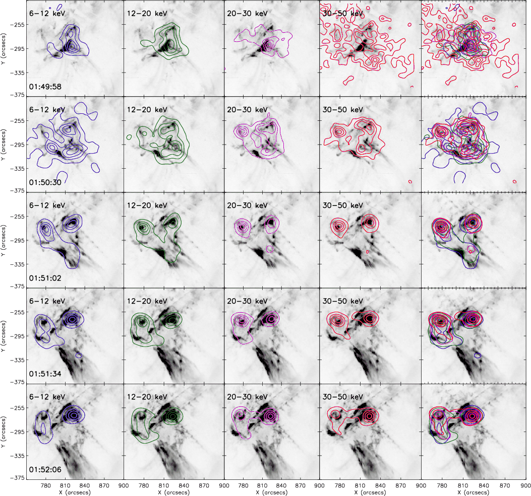
Figure 5: TRACE images with RHESSI image contours overlaid. Rows show time slices at times 01:48:58, 01:50:30, 01:51:02, 01:51:34 and 01:52:06 and columns show contours of RHESSI energy bands at 6-12 (blue), 12-20 (green), 20-30 (magenta) and 30-50 keV (red). The far right column shows all RHESSI contours overlaid. Contour levels are at 90, 75, 50 and 25%. |
| Open with DEXTER | |
From row 2 of Fig. 5,
at time 01:50:30 (hereafter interval 2), emission as high as the
RHESSI 30-50 keV energy band can be seen to be co-spatial with the
jet around (820
![]() ,
-300
,
-300
![]() ).
From the TRACE images this is the region in which we think the twisted
magnetic field became unstable, resulting in the ejection of plasma.
These observations indicate the presence of hard X-rays and hence
non-thermal electrons in the jet, and we believe this to be the first
observation of its kind. Although not shown here, RHESSI images at
these energies with better time resolution have been studied to see how
this source evolves, and on this basis the question of whether the
emission could be from a coronal loop can been dismissed: the hard
X-ray jet emission can be seen to propagate out on a similar time scale
to the ejected material and does not behave like a coronal loop. In
general coronal loops are not present in the early impulsive phase of
the event.
).
From the TRACE images this is the region in which we think the twisted
magnetic field became unstable, resulting in the ejection of plasma.
These observations indicate the presence of hard X-rays and hence
non-thermal electrons in the jet, and we believe this to be the first
observation of its kind. Although not shown here, RHESSI images at
these energies with better time resolution have been studied to see how
this source evolves, and on this basis the question of whether the
emission could be from a coronal loop can been dismissed: the hard
X-ray jet emission can be seen to propagate out on a similar time scale
to the ejected material and does not behave like a coronal loop. In
general coronal loops are not present in the early impulsive phase of
the event.
As the event continues (rows 3, 4 and 5 of Fig. 5)
compact footpoint sources are seen forming at higher energies from
20-50 keV. In the low energy bands sources begin to form,
cospatial with the hot loops faintly visible in TRACE (see also
Fig. 2 (i) onwards), seen as the right hand source in Fig. 5 rows 4 and 5 at roughly (820
![]() ,
-260
,
-260
![]() ).
Note that although these sources appear to be cospatial with the higher
energy sources this is thought to be just a projection effect. For this
paper we concentrate primarily on the emission present in the jet
at 01:50:30.
).
Note that although these sources appear to be cospatial with the higher
energy sources this is thought to be just a projection effect. For this
paper we concentrate primarily on the emission present in the jet
at 01:50:30.
3.2 RHESSI spectroscopy
![\begin{figure}
\par\includegraphics[scale=0.5]{11876f6.ps}
\end{figure}](/articles/aa/full_html/2009/48/aa11876-09/img27.png)
|
Figure 6: RHESSI photon spectra obtained from detector 3 for time interval 2. Black lines shows the background subtracted data and grey shows the background. The plot shows two possible fits, isothermal plus thin target (solid lines) and isothermal plus thick target (dashed lines). Green lines show isothermal fits. Blue lines show thick and thin target fits. Red shows the combined fit functions. Orange shows a Gaussian line added to fit a feature seen at 11 keV. |
| Open with DEXTER | |
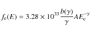
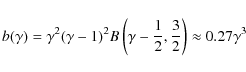
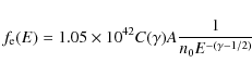
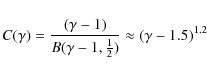
Figure 6 shows the fitted RHESSI spectra obtained from detector 3 for time interval 2. Energy bins of 0.33 keV at lower energies (6-12 keV) were used to properly fit the iron and nickel lines at 6.7 and 8.0 keV. Above 12 keV energy binning of 1 keV was used. The black line shows the background subtracted data and grey the background emission. Figure 6 shows two possible fits to the data between 6-100 keV. Fit 1 is an isothermal (green solid) plus thin target (blue solid) fit to the electron spectrum. Fit 2 is an isothermal (green dashed) plus thick target (blue dashed) fit. The thermal component is characterised by a temperature and an emission measure. The thick and thin target fit functions are characterised by a power law fit to non-thermal electrons between an electron low and a high energy cut off. The electron spectral index and low energy cut off were allowed to vary. Figure 6 shows the conversion to photon spectra and values of temperature, photon spectral index and electron low energy cut off are stated in each plot. An additional Gaussian line (orange) was added to fit the line feature seen at 11 keV. It is thought that this is an instrumental feature but it is not fully understood what is producing this (Dennis 2009, private communication). Red shows the overall combination of fitted functions. Spectral fitting was carried out for individual detectors 1, 3, 4, 6, 8, and 9 and average parameters values calculated. The thermal component is characterised by a temperature of 24 MK and 26 MK for fit 1 and 2 respectively . The hard X-ray spectral index obtained was 4.67 and 4.77 for fit 1 and 2 respectively, thus supporting the evidence for non-thermal electrons present in the event. However using only spatially integrated spectra it is not possible to separate the contribution from the jet and the footpoints and hence it is impossible to determine the spectral parameters resulting from the jet alone, therefore we have carried out imaging spectroscopy.
![\begin{figure}
\par\includegraphics[scale=0.4]{11876f7.ps}
\end{figure}](/articles/aa/full_html/2009/48/aa11876-09/img28.png)
|
Figure 7: RHESSI image at 29.5-37.5 keV ( top left) showing regions chosen for individual spectral analysis. Imaging spectroscopy results for the jet ( top right), left footpoint ( bottom left) and right footpoint ( bottom right). Black lines show the observed photon spectra, green and blue show the isothermal and thick target fit functions respectively. Red shows the combination of fitted functions. |
| Open with DEXTER | |
To perform imaging spectroscopy for time interval 2, images were made using pseudo-logarithmic energy binning from 7.5 keV to 48.5 keV. Despite summing counts from detectors 1, 3, 4, 6, 8 and 9 there were not enough counts for image synthesis above this energy to allow fitting to higher energies. Figure 7 (top left) shows a RHESSI image at 29.5-37.5 keV. Marked on the image are the regions chosen for individual spectral analysis to separate the emission from the jet and the footpoints. Here we fit an isothermal plus broken power fit components to the photon spectrum. For the broken power law component the spectral index below a variable break energy is fixed at 1.5. Above the break the spectral index is allowed to vary. The results are shown in Fig. 7. Black lines show the observed photon spectra, green and blue show the isothermal and broken power law fit functions respectively. Red shows the combination of fitted functions. Stated on each plot are the values obtained for temperature and photon spectral index. We draw particular attention to Fig. 7 (top right) which shows the fitted photon spectrum for the jet characterised by a power law with a spectral index of 4.5 (slightly softer than the value obtained for the footpoints) confirming a non-thermal hard X-ray component in the jet, in turn implying the presence of non-thermal electrons. An estimate of jet temperature was found to be 28 MK. Temperature estimates for the hard X-ray footpoints are stated in each plot. However it should be noted that thermal footpoint emission could be subject to contamination as a result of the bright coronal source contributing to the flux. This is due to side lobes (Krucker & Lin 2002).
![\begin{figure}
\par\includegraphics[angle=90, scale=0.4]{11876f8.ps}
\end{figure}](/articles/aa/full_html/2009/48/aa11876-09/img29.png)
|
Figure 8: NoRH 17 GHz ( top) and 34 GHz ( bottom) images at time intervals used for RHESSI imaging. White lines show positive spectral index from 0.5 to 1.5 in steps of 0.5 corresponding to optically thick plasma. Black lines show lines of negative spectral index from -1 to -4 in steps of 1 corresponding to optically thin plasma. (See electronic version for colour plots.) |
| Open with DEXTER | |
4 Radio observations
4.1 Nobeyama Radioheliograph
The Nobeyama Radioheliograph, a ground-based solar-dedicated radio
interferometer, records full disk images of flux density (brightness)
at 17 and 34 GHz microwave frequencies with spatial
resolution of 10
![]() and 5
and 5
![]() respectively.
During flare events NoRH has an excellent temporal resolution of 0.1s.
Measurements of polarisation are also made at 17 GHz. At these
frequencies the primary solar emission mechanism is gyrosynchrotron.
respectively.
During flare events NoRH has an excellent temporal resolution of 0.1s.
Measurements of polarisation are also made at 17 GHz. At these
frequencies the primary solar emission mechanism is gyrosynchrotron.
Images at 17 GHz (top) and 34 GHz (bottom) are shown in Fig. 8 for the same time intervals as with RHESSI. Note the field of view here is larger than that of Fig. 5
and shows an active region to the north-west of the jet. As time
progresses, ejected material can be seen moving southwest away from the
footpoint region. From the flux at 17 GHz and 34 GHz it is
possible to determine a radio spectral index
![]() from
from
![]() , where
, where
![]() is the flux at frequency
is the flux at frequency ![]() .
Overlaid on the NoRH images are contours of spectral index
.
Overlaid on the NoRH images are contours of spectral index
![]() .
White lines show positive spectral index from 0 to 2 in steps
of 0.5, corresponding to optically thick emission. Black lines
show lines of negative spectral index from -1 to -4 in steps
of 1 corresponding to optically thin emission. As the event progresses
footpoints can be seen forming. At 01:51:34 and onwards these regions
become optically thin. Confirmation of this can be see in Fig. 11
which shows spectra from the Nobeyama Polarimeters from 01:51 onwards.
The turnover in the spectrum occurs at lower frequencies than those
observed by NoRH indicating optically thin emission at 17 GHz and
34 GHz. See Sect. 4.2 for more details. At these frequencies
we can assume that the microwave emission is gyrosynchrotron radiation
from particles at even higher energies than those observed via RHESSI
hard X-rays, and hence definitely non-thermal in nature.
.
White lines show positive spectral index from 0 to 2 in steps
of 0.5, corresponding to optically thick emission. Black lines
show lines of negative spectral index from -1 to -4 in steps
of 1 corresponding to optically thin emission. As the event progresses
footpoints can be seen forming. At 01:51:34 and onwards these regions
become optically thin. Confirmation of this can be see in Fig. 11
which shows spectra from the Nobeyama Polarimeters from 01:51 onwards.
The turnover in the spectrum occurs at lower frequencies than those
observed by NoRH indicating optically thin emission at 17 GHz and
34 GHz. See Sect. 4.2 for more details. At these frequencies
we can assume that the microwave emission is gyrosynchrotron radiation
from particles at even higher energies than those observed via RHESSI
hard X-rays, and hence definitely non-thermal in nature.
We pay particular attention to the images at 01:50:30 (see Fig. 9).
On the left the contours of NoRH 17 GHz (dot-dashed black),
34 GHz (solid blue) and RHESSI 30-50 keV (dashed red) are
overlaid on TRACE. It is important to note that NoRH images are subject
to pointing errors due to random fluctuations of the Earth's
ionosphere, particularly during a flare. Observing the left footpoint
at 17 GHz and 30-50 keV suggests a displacement of 10
![]() in
the E-W direction. Despite this the emission seen by NoRH and
RHESSI are well correlated with each other and with the EUV jet
supporting the evidence for non-thermal particles in the jet at this
time. Figure 9 (right) shows a contour map of spectral index
in
the E-W direction. Despite this the emission seen by NoRH and
RHESSI are well correlated with each other and with the EUV jet
supporting the evidence for non-thermal particles in the jet at this
time. Figure 9 (right) shows a contour map of spectral index
![]() with contours of positive
with contours of positive
![]() ,
ranging from 0
to 1.5 in steps of 0.25. The value of
,
ranging from 0
to 1.5 in steps of 0.25. The value of
![]() for the jetting region is
for the jetting region is ![]() 0.75 corresponding to optically thick emission from the fast-moving electrons.
0.75 corresponding to optically thick emission from the fast-moving electrons.
4.2 Nobeyama polarimeters
In addition to data from the Nobeyama Radioheliograph, radio flux and
polarisation at 1, 2, 3.75, 9.4, 17, 34 and 80 GHz frequencies can
be obtained from the Nobeyama Polarimeters (NoRP). For this event the
flux at 80 GHz remained at the background level and was excluded.
Figure 10 (top) shows a plot of total flux (R+L) and Fig. 10
(middle) shows the degree of circular polarisation (R-L), R and
L denote the right and left circular polarisation. Note that NoRP
records flux from the full disk, however as there appears to be no
other significant activity on the disk during this time interval, the
emission recorded is likely to be from the jet event. It is interesting
to note that the spiky bursts between 01:51:00 and 01:52:00 seen at the
lower frequencies during the impulsive phase have no counterpart at
higher radio frequencies. At 1 GHz these bursts are thought to be
due to plasma emission at the local plasma frequency and its harmonics
caused by a beam of electrons producing Langmuir waves due to a
bump-in-tail instability. The non-linear nature of Langmuir
wave-particle interactions results in the increased flux at 1 GHz.
This effect will also be reflected in the brightness temperature
![]() ,
which can be calculated using the Rayleigh-Jeans law (Eq. (1)) where
,
which can be calculated using the Rayleigh-Jeans law (Eq. (1)) where
![]() is Boltzmann's constant (Dulk 1985).
is Boltzmann's constant (Dulk 1985).

Rearranging Eq. (2) where
![\begin{figure}
\par\includegraphics[width=12cm,clip]{11876f9.ps}
\end{figure}](/articles/aa/full_html/2009/48/aa11876-09/img43.png)
|
Figure 9:
Left: TRACE image with NoRH 17 GHz (dot-dashed black),
34 GHz (solid blue) and RHESSI 30-50 keV (dashed red)
contours. Contour levels of 90, 75, 50% for all contours (plus 25% for
17 GHz and 30-50 keV). Right: Map of radio spectral index |
| Open with DEXTER | |
In the text
![\begin{figure}
\par\includegraphics[scale=0.4]{11876f10.ps}
\end{figure}](/articles/aa/full_html/2009/48/aa11876-09/img44.png)
|
Figure 10: Top: NoRP flux (R+L) at 1, 2, 3.75, 9.4, 17 and 34 GHz. Middle: NoRP flux (R-L) showing degree of circular polarisation. Bottom: brightness temperature calculated at each frequency. The dashed vertical lines show time intervals over which RHESSI images were obtained for Fig. 5. |
| Open with DEXTER | |
Figure 11 shows plots of
NoRP radio spectra following the evolution of the event beginning
01:51:00. Before this the flux at higher frequencies is still at the
level of the background. The spectra are made by summing the flux over
15 s time intervals and normalising. Error bars at the 10%
level are assigned to the data points as an estimate of errors due to
atmospheric effects and local weather conditions. The spectra were then
fitted using a function for gyrosynchrotron emission (Eq. (3)) allowing for four fit parameters (see http://solar.nro.nao.ac.jp/norp/ for details):
![]() ,
the positive power index at low frequencies (corresponding to optically thick plasma),
,
the positive power index at low frequencies (corresponding to optically thick plasma),
![]() is the negative power index at high frequencies corresponding to optically thin plasma,
is the negative power index at high frequencies corresponding to optically thin plasma,
![]() the turn-over frequency and
the turn-over frequency and
![]() the turn-over flux
density.
the turn-over flux
density.
To fit the data we used the standard NoRP software which first chooses
Plasma emission is at the local electron plasma frequency
![]() or its second harmonic
or its second harmonic
![]() which is dependent on the plasma density n. Figure 12 (http://sunbase.nict.go.jp/solar/denpa/hirasDB/Events/)
shows a radio spectrogram from the Hiraiso Solar Observatory (HiRAS)
which observes in the range 25-2500 MHz. The spectrogram shows
faint type III bursts starting
which is dependent on the plasma density n. Figure 12 (http://sunbase.nict.go.jp/solar/denpa/hirasDB/Events/)
shows a radio spectrogram from the Hiraiso Solar Observatory (HiRAS)
which observes in the range 25-2500 MHz. The spectrogram shows
faint type III bursts starting ![]() 01:50:50 followed by more intense bursts at
01:50:50 followed by more intense bursts at ![]() 01:51:30.
The spectrogram shows high frequency type III bursts which have a
duration of about a minute during which the frequency drifts from
01:51:30.
The spectrogram shows high frequency type III bursts which have a
duration of about a minute during which the frequency drifts from ![]() 1800 MHz to
1800 MHz to ![]() 400 MHz
due to decreasing plasma density as the beam propagates out. This
confirms that the bursts detected at 1 GHz by NoRP is indeed
plasma emission. At lower frequencies, more intense type III
emission can be seen lasting around
400 MHz
due to decreasing plasma density as the beam propagates out. This
confirms that the bursts detected at 1 GHz by NoRP is indeed
plasma emission. At lower frequencies, more intense type III
emission can be seen lasting around
![]() min which drifts to frequencies below the observing range of HiRAS. Figure 13
shows a spectrogram obtained from RAD2 on the WAVES experiment on the
WIND satellite which observes in the range 1.075-13.825 MHz (Bougeret et al. 1995). Figure 13
shows that the type III emission continues to drift to frequencies
as low as 1 MHz. From the starting frequency of the radio bursts
it is possible to determine the local plasma density n and from this estimate a height at which the burst was emitted. Using
min which drifts to frequencies below the observing range of HiRAS. Figure 13
shows a spectrogram obtained from RAD2 on the WAVES experiment on the
WIND satellite which observes in the range 1.075-13.825 MHz (Bougeret et al. 1995). Figure 13
shows that the type III emission continues to drift to frequencies
as low as 1 MHz. From the starting frequency of the radio bursts
it is possible to determine the local plasma density n and from this estimate a height at which the burst was emitted. Using
![]() as an approximate starting frequency of the plasma emission, then we can estimate n to be a few
as an approximate starting frequency of the plasma emission, then we can estimate n to be a few
![]() .
If we assume that the type III radio burst is caused within the
jet this suggests that the jet density is consistent with low coronal
density.
.
If we assume that the type III radio burst is caused within the
jet this suggests that the jet density is consistent with low coronal
density.
![\begin{figure}
\par\includegraphics[scale=0.37]{11876f11.ps}
\end{figure}](/articles/aa/full_html/2009/48/aa11876-09/img60.png)
|
Figure 11:
NoRP radio spectra at 15 s time intervals. Solid line shows
gyrosynchrotron function fitted to the data from 1 to 34 GHz.
Dashed line shows the same function fitted to data from 2 to
34 GHz. Corresponding values of
|
| Open with DEXTER | |
![\begin{figure}
\par\includegraphics[scale=0.27]{11876f12.ps}
\end{figure}](/articles/aa/full_html/2009/48/aa11876-09/img61.png)
|
Figure 12: Radio spectrogram from the Hiraiso solar observatory (25-2500 MHz) showing type III radio bursts. (See electronic version for colour plots.) |
| Open with DEXTER | |
5 Discussion and conclusion
The evolution of the jet observed on the 22 August 2002 is similar to that of events described by Shimojo et al. (2007)
in which a twisted loop rises prior to the jet. The evolution can be
compared to that described by the magnetic reconnection jet of e.g. Shimojo et al. (1996); Heyvaerts et al. (1977).
Reconnection with the overlying coronal field results in field
reconfiguration and the ejection of hot X-ray emitting plasma. As the
event progresses TRACE observations show loops forming at the base of
the jet as expected by the magnetic reconnection model. In addition to
this the ejected material appears to untwist slightly as twist from the
emerging field is transferred to the ``open'' field lines of the jet.
We found an apparent jet velocity of ![]() 500
500
![]() which is consistent with predictions of velocities on the order of the
Alfvén speed for this model. Calculating the Alfvén speed,
which is consistent with predictions of velocities on the order of the
Alfvén speed for this model. Calculating the Alfvén speed,
![]() for B=10 G and
for B=10 G and
![]() we obtain
we obtain
![]() .
However it should be noted that for plasma temperatures such as those
found from RHESSI spectroscopy the sound speed in the corona will be in
the range of
.
However it should be noted that for plasma temperatures such as those
found from RHESSI spectroscopy the sound speed in the corona will be in
the range of
![]() .
.
At the time of the main ejection RHESSI imaging shows hard X-rays to as
high as 30-50 keV present in the jet. This is the first time that
hard X-rays coming from the jet location have been reported. Sui et al. (2006)
have reported an event which may demonstrate hard X-ray emission from a
jet region, a 6-12 keV coronal source was observed in the vicinity
of a cusp-like, possibly jetting, structure above the apex of a compact
flare loop. However without imaging spectroscopy it was not possible to
determine if the source was thermal or non-thermal. Krucker et al. (2008)
found evidence for non-thermal coronal X-rays in the 14-30 keV
range at the onset time of an interplanetary type III radio burst,
suggesting emission by escaping fast electrons, however there was no
radio or other coronal imaging of a jet or other feature supporting
this interpretation. By contrast, our observations show a clear spatial
as well as temporal association of the jet with the non-thermal
emission in both radio and hard X-rays, and therefore we believe this
to be the first clear observation of non-thermal emission from
flare-accelerated escaping electrons. RHESSI imaging spectroscopy
includes a broken power law fit function which yields a spectral index
of ![]() 4.5 confirming the presence of non-thermal jet electrons.
4.5 confirming the presence of non-thermal jet electrons.
If the non-thermal emission is bremsstrahlung caused by electrons
propagating in a thick target coronal source in the jet then we can
estimate the number of electrons above 20 keV using Eqs. (4), (5) and (6)
where
where
| Figure 13: Spectrogram from WAVES on the WIND spacecraft (1.075-13.825 MHz) showing type III radio bursts. |
|
| Open with DEXTER | |
In addition, RHESSI spectral fitting suggests a jet temperature of ![]()
![]() .
As no hot loops are seen in this region with TRACE at this time or
slightly after we are confident that this indeed the temperature of the
jet. As suggested by Feldman et al. (1999),
at these high temperatures the thermal continuum from free-free and
free-bound emission will be significant. From this it is plausible to
suggest that TRACE images reveal free-free emission in the jet similar
to that observed with RHESSI. NoRH observations at 17 and
34 GHz are seen to be co-spatial with the hard X-ray emission
during this time and
.
As no hot loops are seen in this region with TRACE at this time or
slightly after we are confident that this indeed the temperature of the
jet. As suggested by Feldman et al. (1999),
at these high temperatures the thermal continuum from free-free and
free-bound emission will be significant. From this it is plausible to
suggest that TRACE images reveal free-free emission in the jet similar
to that observed with RHESSI. NoRH observations at 17 and
34 GHz are seen to be co-spatial with the hard X-ray emission
during this time and ![]() is found to be
is found to be ![]() 0.75
corresponding to optically thick emission by non-thermal electrons,
reinforcing our claim that that X-rays are directly revealing the
presence of these particles in the jet. Further radio observations from
NoRP and HiRAS show simultaneous bursts of plasma emission at
0.75
corresponding to optically thick emission by non-thermal electrons,
reinforcing our claim that that X-rays are directly revealing the
presence of these particles in the jet. Further radio observations from
NoRP and HiRAS show simultaneous bursts of plasma emission at
![]() .
If we assume this results from a beam of electronsaccelerated in the jet, we calculate
.
If we assume this results from a beam of electronsaccelerated in the jet, we calculate
![]() which is a reasonable jet density. We believe this to be a rare
observation, but one lending strong support to a model involving
coronal electron acceleration in a relatively dense plasma and in close
association with the magnetic reconfiguration that launches the jet.
which is a reasonable jet density. We believe this to be a rare
observation, but one lending strong support to a model involving
coronal electron acceleration in a relatively dense plasma and in close
association with the magnetic reconfiguration that launches the jet.
H.M.B. gratefully acknowledges the support of an STFC studentship. L.F. gratefully acknowledges the support of an STFC Rolling Grant, and financial support by the European Commission through the SOLAIRE Network (MTRN-CT_2006-035484). We would like to thank Brian Dennis for useful comments regarding RHESSI spectral fitting. We would like to also thank NoRH and NoRP teams for help regarding radio analysis, and an anonymous referee whose suggestions helped us to improve this paper.
References
- Alexander, D., & Fletcher, L. 1999, Sol. Phys., 190, 167 [NASA ADS] [CrossRef]
- Aschwanden, M. J., Nightingale, R. W., Tarbell, T. D., & Wolfson, C. J. 2000, Astrophys. J., 535, 1027 [NASA ADS] [CrossRef]
- Bougeret, J.-L., Kaiser, M. L., Kellogg, P. J., et al. 1995, Space Sci. Rev., 71, 231 [NASA ADS] [CrossRef]
- Brown, J. C. 1971, Sol. Phys., 18, 489 [NASA ADS] [CrossRef]
- Canfield, R. C., Reardon, K. P., Leka, K. D., et al. 1996, ApJ, 464, 1016 [NASA ADS] [CrossRef]
- Chifor, C., Young, P. R., Isobe, H., et al. 2008, A&A, 481, L57 [NASA ADS] [EDP Sciences] [CrossRef]
- Christe, S., Krucker, S., & Lin, R. P. 2008, ApJ, 680, L149 [NASA ADS] [CrossRef]
- Dulk, G. A. 1985, ARA&A, 23, 169 [NASA ADS] [CrossRef]
- Feldman, U., Laming, J. M., Doschek, G. A., Warren, H. P., & Golub, L. 1999, ApJ, 511, L61 [NASA ADS] [CrossRef]
- Golub, L., Deluca, E., Austin, G., et al. 2007, Sol. Phys., 243, 63 [NASA ADS] [CrossRef]
- Handy, B. N., Acton, L. W., Kankelborg, C. C., et al. 1999, Sol. Phys., 187, 229 [NASA ADS] [CrossRef]
- Heyvaerts, J., Priest, E. R., & Rust, D. M. 1977, ApJ, 216, 123 [NASA ADS] [CrossRef]
- Hudson, H. S., Canfield, R. C., & Kane, S. R. 1978, Sol. Phys., 60, 137 [NASA ADS] [CrossRef]
- Krucker, S., & Lin, R. P. 2002, Sol. Phys., 210, 229 [NASA ADS] [CrossRef]
- Krucker, S., Saint-Hilaire, P., Christe, S., et al. 2008, ApJ, 681, 644 [NASA ADS] [CrossRef]
- Lin, R. P., Dennis, B. R., et al. 2002, Sol. Phys., 210, 3 [NASA ADS] [CrossRef]
- Moreno-Insertis, F., Galsgaard, K., & Ugarte-Urra, I. 2008, ApJ, 673, L211 [NASA ADS] [CrossRef]
- Nakajima, H., Nishio, M., Enome, S., et al. 1994, IEEE Proc., 82, 705 [NASA ADS] [CrossRef]
- Nishizuka, N., Shimizu, M., Nakamura, T., et al. 2008, ApJ, 683, L83 [NASA ADS] [CrossRef]
- Pariat, E., Antiochos, S. K., & DeVore, C. R. 2009, ApJ, 691, 61 [NASA ADS] [CrossRef]
- Savcheva, A., Cirtain, J., Deluca, E. E., et al. 2007, PASJ, 59, 771 [NASA ADS]
- Shibata, K., & Uchida, Y. 1986, Sol. Phys., 103, 299 [NASA ADS] [CrossRef]
- Shibata, K., Ishido, Y., Acton, L. W., et al. 1992, PASJ, 44, L173 [NASA ADS] [CrossRef]
- Shibata, K., Nitta, N., Strong, K. T., et al. 1994, ApJ, 431, L51 [NASA ADS] [CrossRef]
- Shimojo, M., & Shibata, K. 2000, ApJ, 542, 1100 [NASA ADS] [CrossRef]
- Shimojo, M., Hashimoto, S., Shibata, K., et al. 1996, PASJ, 48, 123 [NASA ADS]
- Shimojo, M., Narukage, N., Kano, R., et al. 2007, PASJ, 59, 745
- Sterling, A. C., Shibata, K., & Mariska, J. T. 1993, ApJ, 407, 778 [NASA ADS] [CrossRef]
- Strong, K. T., Harvey, K., Hirayama, T., et al. 1992, PASJ, 44, L161 [NASA ADS]
- Sui, L., Holman, G. D., & Dennis, B. R. 2006, ApJ, 646, 605 [NASA ADS] [CrossRef]
- Torii, C., Tsukiji, Y., Kobayashi, S., et al. 1979, Nagoya University, Research Institute of Atmospherics, Proceedings, 26, 129
- Török, T., & Kliem, B. 2005, ApJ, 630, L97 [NASA ADS] [CrossRef]
- Tsuneta, S., Acton, L., Bruner, M., et al. 1991, Sol. Phys., 136, 37 [NASA ADS] [CrossRef]
- Uchida, Y. 1969, PASJ, 21, 128 [NASA ADS]
- Yokoyama, T., & Shibata, K. 1995, Nature, 375, 42 [NASA ADS] [CrossRef]
All Figures
|
|
Figure 1: From top to bottom: GOES, RHESSI, TRACE and NoRH lightcurves. Vertical dashed lines represent 32 s time intervals used for RHESSI imaging (see Fig. 5). (See electronic version for colour plots.) |
| Open with DEXTER | |
| In the text | |
|
|
Figure 2:
TRACE 195Å images for selected times throughout the event showing
the evolution of the jet. These images have a time resolution of |
| Open with DEXTER | |
| In the text | |
|
|
Figure 3: Velocity timeslice showing jet intensity as a function of height and time. Vertical dash-dot line shows the time at which the jet emission passes out of the TRACE field of view. Dashed lines on insert image show the region used for the analysis. Asterisks and solid line shows a fit to the faint front edge of the jet at the 5% level. Diamonds and dashed line shows a fit to points determined from tracking a brightly emitting source of plasma by eye. |
| Open with DEXTER | |
| In the text | |
| |
Figure 4: RHESSI lightcurve with logarithmic energy binning. Vertical dashed lines represent 32 s time intervals used for RHESSI imaging (see Fig. 5). (See electronic version for colour plots.) |
| Open with DEXTER | |
| In the text | |
|
|
Figure 5: TRACE images with RHESSI image contours overlaid. Rows show time slices at times 01:48:58, 01:50:30, 01:51:02, 01:51:34 and 01:52:06 and columns show contours of RHESSI energy bands at 6-12 (blue), 12-20 (green), 20-30 (magenta) and 30-50 keV (red). The far right column shows all RHESSI contours overlaid. Contour levels are at 90, 75, 50 and 25%. |
| Open with DEXTER | |
| In the text | |
|
|
Figure 6: RHESSI photon spectra obtained from detector 3 for time interval 2. Black lines shows the background subtracted data and grey shows the background. The plot shows two possible fits, isothermal plus thin target (solid lines) and isothermal plus thick target (dashed lines). Green lines show isothermal fits. Blue lines show thick and thin target fits. Red shows the combined fit functions. Orange shows a Gaussian line added to fit a feature seen at 11 keV. |
| Open with DEXTER | |
| In the text | |
|
|
Figure 7: RHESSI image at 29.5-37.5 keV ( top left) showing regions chosen for individual spectral analysis. Imaging spectroscopy results for the jet ( top right), left footpoint ( bottom left) and right footpoint ( bottom right). Black lines show the observed photon spectra, green and blue show the isothermal and thick target fit functions respectively. Red shows the combination of fitted functions. |
| Open with DEXTER | |
| In the text | |
|
|
Figure 8: NoRH 17 GHz ( top) and 34 GHz ( bottom) images at time intervals used for RHESSI imaging. White lines show positive spectral index from 0.5 to 1.5 in steps of 0.5 corresponding to optically thick plasma. Black lines show lines of negative spectral index from -1 to -4 in steps of 1 corresponding to optically thin plasma. (See electronic version for colour plots.) |
| Open with DEXTER | |
| In the text | |
|
|
Figure 9:
Left: TRACE image with NoRH 17 GHz (dot-dashed black),
34 GHz (solid blue) and RHESSI 30-50 keV (dashed red)
contours. Contour levels of 90, 75, 50% for all contours (plus 25% for
17 GHz and 30-50 keV). Right: Map of radio spectral index |
| Open with DEXTER | |
| In the text | |
|
|
Figure 10: Top: NoRP flux (R+L) at 1, 2, 3.75, 9.4, 17 and 34 GHz. Middle: NoRP flux (R-L) showing degree of circular polarisation. Bottom: brightness temperature calculated at each frequency. The dashed vertical lines show time intervals over which RHESSI images were obtained for Fig. 5. |
| Open with DEXTER | |
| In the text | |
|
|
Figure 11:
NoRP radio spectra at 15 s time intervals. Solid line shows
gyrosynchrotron function fitted to the data from 1 to 34 GHz.
Dashed line shows the same function fitted to data from 2 to
34 GHz. Corresponding values of
|
| Open with DEXTER | |
| In the text | |
|
|
Figure 12: Radio spectrogram from the Hiraiso solar observatory (25-2500 MHz) showing type III radio bursts. (See electronic version for colour plots.) |
| Open with DEXTER | |
| In the text | |
| |
Figure 13: Spectrogram from WAVES on the WIND spacecraft (1.075-13.825 MHz) showing type III radio bursts. |
| Open with DEXTER | |
| In the text | |
Copyright ESO 2009
Current usage metrics show cumulative count of Article Views (full-text article views including HTML views, PDF and ePub downloads, according to the available data) and Abstracts Views on Vision4Press platform.
Data correspond to usage on the plateform after 2015. The current usage metrics is available 48-96 hours after online publication and is updated daily on week days.
Initial download of the metrics may take a while.