| Issue |
A&A
Volume 508, Number 3, December IV 2009
|
|
|---|---|---|
| Page(s) | 1099 - 1116 | |
| Section | Astrophysical processes | |
| DOI | https://doi.org/10.1051/0004-6361/200809830 | |
| Published online | 27 October 2009 | |
A&A 508, 1099-1116 (2009)
Positron transport in the interstellar medium
P. Jean1 - W. Gillard1,2,3 - A. Marcowith4 - K. Ferrière5
1 - CESR, Université de Toulouse, CNRS, INSU: 9 avenue du colonel Roche, BP 44346, 31028 Toulouse, France
2 -
KTH, Department of Physics, AlbaNova University Centre, 10691 Stockholm, Sweden
3 -
The Oskar Klein Centre for Cosmo Particle Physics, AlbaNova, 10691 Stockholm, Sweden
4 - LPTA, CNRS, Université Montpellier II, 34095 Montpellier Cedex 5, France
5 -
LATT, Université de Toulouse, CNRS: 14 avenue Édouard Belin, 31400 Toulouse, France
Received 22 March 2008 / Accepted 22 September 2009
Abstract
Aims. We seek to understand the propagation mechanisms of
positrons in the interstellar medium (ISM). This understanding is a key
to determine whether the spatial distribution of the annihilation
emission observed in our Galaxy reflects the spatial distribution of
positron sources and, therefore, makes it possible to place constraints
on the origin of positrons.
Methods. We review the different processes that are likely to
affect the transport of positrons in the ISM. These processes fall into
three broad categories: scattering off magnetohydrodynamic waves,
collisions with particles of the interstellar gas, and advection with
large-scale fluid motions. We assess the efficiency of each process and
describe its impact on the propagation of positrons. We also develop a
model of positron propagation, based on Monte-Carlo simulations, which
enable us to estimate the distances traveled by positrons in the
different phases of the ISM.
Results. We find that low-energy (
![]() )
positrons generally have negligible interactions with
magnetohydrodynamic waves, insofar as these waves are heavily damped.
Positron propagation is mainly controlled by collisions with gas
particles. Under these circumstances, positrons can travel very large
distances (up to
)
positrons generally have negligible interactions with
magnetohydrodynamic waves, insofar as these waves are heavily damped.
Positron propagation is mainly controlled by collisions with gas
particles. Under these circumstances, positrons can travel very large
distances (up to
![]() for 1 MeV positrons) along magnetic field lines before annihilating.
for 1 MeV positrons) along magnetic field lines before annihilating.
Key words: gamma rays: theory - diffusion - plasmas
1 Introduction
Positron annihilation in the Galactic center (GC) region is now a firmly established source of radiation, which has been observed since the early seventies in several balloon and satellite experiments (see von Ballmoos et al. 2003; Jean et al. 2004; Diehl et al. 2006 for reviews). Despite significant progress in observational capabilities, the origin of Galactic positrons remains an open question.
Recent observations of the 511 keV line intensity using the SPI
spectrometer onboard the International Gamma-Ray Laboratory
(INTEGRAL) observatory have revealed a diffuse emission, distributed in
the bulge and the disk of our Galaxy
(Knödlseder et al. 2005; Weidenspointner et al. 2006). Observations further
indicate that the bulge-to-disk luminosity ratio
(hereafter B/D) of the 511 keV line is rather large (![]() 3-9)
compared to the distribution of any candidate source. Under the
hypothesis that positrons annihilate close to their sources, the
spatial distribution of the annihilation emission should reflect
the spatial distribution of the positron sources. In this view, the large
B/D ratio could be explained by sources belonging to
the old stellar population (Knödlseder et al. 2005) and a disk
emission, partly or totally, attributed to the radioactive
decay of 26Al and 44Ti produced in massive stars. The most
recent SPI analysis covering more than 4 years of data shows hints
of a longitudinal asymmetry in the spatial distribution of
the 511 keV line emission produced in the
inner part of the Galactic disk (Weidenspointner et al. 2008).
A similar asymmetry is observed in the distribution of low-mass
X-ray binaries emitting at high energies, suggesting that these objects
might be the dominant sources of positrons. This conclusion is
contingent upon the hypothesis that positrons annihilate close to their
sources, a hypothesis that should be called into question.
3-9)
compared to the distribution of any candidate source. Under the
hypothesis that positrons annihilate close to their sources, the
spatial distribution of the annihilation emission should reflect
the spatial distribution of the positron sources. In this view, the large
B/D ratio could be explained by sources belonging to
the old stellar population (Knödlseder et al. 2005) and a disk
emission, partly or totally, attributed to the radioactive
decay of 26Al and 44Ti produced in massive stars. The most
recent SPI analysis covering more than 4 years of data shows hints
of a longitudinal asymmetry in the spatial distribution of
the 511 keV line emission produced in the
inner part of the Galactic disk (Weidenspointner et al. 2008).
A similar asymmetry is observed in the distribution of low-mass
X-ray binaries emitting at high energies, suggesting that these objects
might be the dominant sources of positrons. This conclusion is
contingent upon the hypothesis that positrons annihilate close to their
sources, a hypothesis that should be called into question.
Several authors have argued that positrons annihilate in the vicinity
of their production sites, based on the assumption that particles
propagate according to the so-called Bohm diffusion, i.e., with a
mean free-path equal to their Larmor radius (Boehm et al. 2004; Wang 2006).
This implicitly supposes that magnetic fluctuations in the ISM
are strongly tangled on all scales, as is likely the case near strong
shocks in supernova remnants. In reality,
given the complexity and the variety of thermodynamical phases
in the ISM, Bohm diffusion probably
overestimates particle confinement (Parizot et al. 2004a).
Jean et al. (2006) estimated the distances traveled by positrons using
a model combining a quasi-linear diffusion theory of wave-particle
interactions at high energy and an approximate propagation model
including collisions
with the ambient ISM matter at low energy. A preliminary model of the gas
content in the Galactic bulge (a more complete description of the gas
spatial distribution in this region is presented in Ferrière et al. 2007)
was then added to the propagation model. The authors concluded that MeV
positrons injected by radioactive processes into the bulge cannot escape
from it and that a single source releasing positrons in the bulge
might have difficulties accounting for the observed spatial extent of
the annihilation emission. Prantzos (2006) proposed a solution
to explain the large B/D ratio measured with SPI, in which
positrons produced by type Ia supernovae in the old disk are
transported along magnetic field lines into the bulge. Cheng et al. (2006)
suggested that positrons in the bulge could originate from
the decay of ![]() produced in high-energy pp collisions. In this work,
the energetic protons would be shock-accelerated when a star is tidally disrupted
in the accretion disk of Sagittarus A
produced in high-energy pp collisions. In this work,
the energetic protons would be shock-accelerated when a star is tidally disrupted
in the accretion disk of Sagittarus A![]() (
(
![]() ). Since high-energy
(>30 MeV) positrons take as long as
). Since high-energy
(>30 MeV) positrons take as long as
![]() years to cool down, they
should be able to propagate far away from
years to cool down, they
should be able to propagate far away from
![]() and to fill the Galactic
bulge. In order to explain the annihilation emission in the bulge,
Totani (2006) proposed a scenario in which MeV positrons were
produced in the accretion disk of
and to fill the Galactic
bulge. In order to explain the annihilation emission in the bulge,
Totani (2006) proposed a scenario in which MeV positrons were
produced in the accretion disk of
![]()
![]() years ago. These
positrons would have filled the bulge while being transported by
large-scale outflows (
years ago. These
positrons would have filled the bulge while being transported by
large-scale outflows (![]() 100 km s-1). All these studies invoked
positron transport to explain the observed annihilation emission, but
they did not include any detailed examination of the physical processes
that could contribute to it.
100 km s-1). All these studies invoked
positron transport to explain the observed annihilation emission, but
they did not include any detailed examination of the physical processes
that could contribute to it.
More recently, Higdon et al. (2009) discussed the role of magnetohydrodynamical (MHD) fluctuations in positron transport in the different ISM phases. They further estimated the positron mean free path using a phenomenological model of MeV electron transport in interplanetary turbulence, especially in the ionized phases where turbulence is undamped down to small scales (see appendix). However, the model used to derive the positron mean free-path is strictly valid for interplanetary plasmas, and the nature of ISM turbulence is likely different. The model developed by Higdon et al. (2009) is up to now the most valuable attempt to account for the propagation of low-energy positrons in the ISM. Here, rather than considering a particular turbulent model, we review the transport processes that govern the positron mean free path.
We discuss three different regimes of positron transport in the Galaxy, namely, the regime dominated by scattering off MHD waves (Sect. 2), the regime dominated by collisions with particles of the interstellar gas (Sect. 3) and a regime of advection with large-scale fluid motion (Sect. 4). Based on the quantitative results obtained in each section, we infer the relevance and the importance of the respective regimes. In Sect. 5, we summarize our study and discuss its possible implications for positron transport at Galactic scales.
2 Scattering off magnetohydrodynamic waves
In Sect. 2.1, we present the condition for wave-particle resonance, restricting our analysis to magnetohydrodynamic (MHD) waves. We further discuss the effective value of the Alfvén speed in the neutral phases of the ISM. In Sect. 2.2, we present the properties of the MHD wave cascades initiated at large spatial scales, e.g., by the differential rotation of the Galaxy or by the explosion of supernovae. In Sect. 2.2.1, we present the different energy transfer times associated with the different type of cascades that likely developped in the ISM. In Sect. 2.2.2, we discuss the collisional and collisionless damping mechanisms of MHD waves as well as the smallest scales of the MHD cascades in the different ISM phases. Only a brief summary is given there; the technical derivation is postponed to Appendix A. In Sect. 2.3, we discuss the global effect on positron transport of MHD waves injected at large scales. In Sect. 2.4, we consider the local effect of magnetic fluctuations generated by the streaming instability, which can survive down to the small scales of low-energy positrons.
Throughout Sect. 2, we assume, for simplicity, that the interstellar gas contains only hydrogen.
2.1 Positron resonance with MHD waves
In a medium with non-vanishing magnetic field, wave-particle
interactions proceed through the Landau-synchrotron resonance
condition expressed as (Melrose 1986):
where
In this work, we consider only MHD waves, more specifically, shear
Alfvén waves and fast magnetosonic waves as these waves are a major part of the
magnetic fluctuations that pervade the ISM (Lithwick & Goldreich 2001). We do not consider slow
waves separately, because the dynamics of the slow wave cascade were
shown to be entirely controlled by the Alfvén wave cascade
(Lithwick & Goldreich 2001) and the slow wave spectrum is basically
the same as the Alfvén wave spectrum. Following Yan & Lazarian (2004), we
assume that the transport of charged particles is governed
by either Alfvén waves or fast magnetosonic waves. Note that
higher-frequency waves are potentially important as well, as they can
easily fulfill the above resonance condition with positrons produced
by radioactive decay (energy
![]() ).
However, whistler waves, the most interesting waves in this frequency
domain, are right-handed polarized and, therefore, cannot be in
resonance with positrons. Higdon et al. (2009) have discussed
the possible role of self-generated whistler waves. We will come back
to this
possibility in Sect. 2.4. The possible effects of
large-scale compressible
motion will be examined in Sect. 4.
).
However, whistler waves, the most interesting waves in this frequency
domain, are right-handed polarized and, therefore, cannot be in
resonance with positrons. Higdon et al. (2009) have discussed
the possible role of self-generated whistler waves. We will come back
to this
possibility in Sect. 2.4. The possible effects of
large-scale compressible
motion will be examined in Sect. 4.
For the waves of interest here, it can be shown that
![]()
![]() , so we are entitled to neglect
, so we are entitled to neglect ![]() in
Eq. (1), except in the particular case
in
Eq. (1), except in the particular case ![]() .
The
case
.
The
case ![]() corresponds to the so-called Cherenkov resonance, in
which the particle interacts with a zero-frequency wave in a frame
moving at velocity
corresponds to the so-called Cherenkov resonance, in
which the particle interacts with a zero-frequency wave in a frame
moving at velocity
![]() .
In that case, Eq. (1)
reduces to
.
In that case, Eq. (1)
reduces to
![]() .
The Cherenkov
resonance can be important for magnetosonic waves, which have a
perturbed magnetic field component parallel to the background
magnetic field.
.
The Cherenkov
resonance can be important for magnetosonic waves, which have a
perturbed magnetic field component parallel to the background
magnetic field.
Table 1: Physical parameters of the different ISM phases.
Here, we consider only the dominant harmonics
![]() .
With
.
With
![]() ,
Eq. (1) can then be recast
into the form
,
Eq. (1) can then be recast
into the form
where
or in terms of the particle kinetic energy,
![\begin{displaymath}
\ensuremath{E_{k}} = (m_{\rm e} ~ c^2) \ \left[\sqrt{\left(\...
...B}{m_{\rm
e}c^2~k_\parallel~\cos\alpha}\right)^2+1}-1\right] .
\end{displaymath}](/articles/aa/full_html/2009/48/aa09830-08/img65.png)
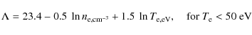
Roughly speaking, MHD waves can exist only at frequencies lower than the proton cyclotron frequency,

Either they are damped by collisional effects (mainly viscous friction and ion-neutral collisions) at low frequencies (see Sect. A.1) or, if they manage to survive collisional effects, then at frequencies approaching
For Alfvén waves (
![]() ,
with
,
with ![]() the Alfvén speed), Eq. (5) is equivalent to
the Alfvén speed), Eq. (5) is equivalent to

which, in view of the resonance conditions, Eqs. (3) and (4), implies a threshold on the positron momentum (obtained for

and a threshold on the positron kinetic energy:
![\begin{displaymath}
\ensuremath{E_{k}}\ge (m_{\rm e} ~ c^2) \
\left[
\sqrt{
\l...
... ~ V_{\rm A}}
{m_{\rm e} ~ c}
\right)^2 + 1
} - 1
\right] .
\end{displaymath}](/articles/aa/full_html/2009/48/aa09830-08/img74.png)
For fast magnetosonic waves (

and the thresholds on the positron momentum and kinetic energy (again obtained for

and
![\begin{displaymath}
\ensuremath{E_{k}}\ge (m_{\rm e} ~ c^2) \
\left[
\sqrt{
\l...
...V_{\rm F}(0)}
{m_{\rm e} ~ c}
\right)^2 + 1
} - 1
\right] ,
\end{displaymath}](/articles/aa/full_html/2009/48/aa09830-08/img88.png)
respectively.
The question now is what expression should be used for the Alfvén
speed. In a fully ionized medium, the Alfvén speed is simply
![]() ,
with
,
with
![]() the
ion mass density. However, in a partially ionized medium, the
relevant Alfvén speed depends on the degree of coupling between
ions and neutrals. If the ion-neutral and neutral-ion collision
frequencies,
the
ion mass density. However, in a partially ionized medium, the
relevant Alfvén speed depends on the degree of coupling between
ions and neutrals. If the ion-neutral and neutral-ion collision
frequencies,
![]() and
and
![]() ,
are much greater than
the wave frequency,
,
are much greater than
the wave frequency, ![]() ,
then ions and neutrals are very well
coupled through ion-neutral collisions, and as a result, an
Alfvén wave will set the entire fluid (ions + neutrals) into
motion. In that case, one should use the total Alfvén speed,
,
then ions and neutrals are very well
coupled through ion-neutral collisions, and as a result, an
Alfvén wave will set the entire fluid (ions + neutrals) into
motion. In that case, one should use the total Alfvén speed,
![]() ,
with
,
with
![]() the total (ion + neutral) mass
density. In contrast, if the ion-neutral and neutral-ion collision
frequencies are much smaller than the wave frequency, then ions and
neutrals are no longer coupled, and an Alfvén wave will set the
ions alone in motion. In that case, one should use the
ionic Alfvén speed,
the total (ion + neutral) mass
density. In contrast, if the ion-neutral and neutral-ion collision
frequencies are much smaller than the wave frequency, then ions and
neutrals are no longer coupled, and an Alfvén wave will set the
ions alone in motion. In that case, one should use the
ionic Alfvén speed,
![]() ,
as in a fully ionized medium.
,
as in a fully ionized medium.
In an atomic medium with temperature ![]() K, the
ion-neutral and neutral-ion collision frequencies are given by
K, the
ion-neutral and neutral-ion collision frequencies are given by
![]() and
and
![]() ,
where
,
where ![]() and
and ![]() are the neutral and ion number
densities, respectively (Osterbrock 1961). At high
temperature, the collision frequencies increase as
are the neutral and ion number
densities, respectively (Osterbrock 1961). At high
temperature, the collision frequencies increase as ![]() (Braginskii 1965; Shull & Draine 1987); assuming an effective
cross section for H-H+ collisions
(Braginskii 1965; Shull & Draine 1987); assuming an effective
cross section for H-H+ collisions
![]() (Wentzel 1974), we find that, for
(Wentzel 1974), we find that, for ![]() K,
K,
![]() and
and
![]() .
In a molecular
medium, the collision frequencies are
.
In a molecular
medium, the collision frequencies are
![]() and
and
![]() (Osterbrock 1961). For comparison, the frequency of a
resonant Alfvén wave is given by
(Osterbrock 1961). For comparison, the frequency of a
resonant Alfvén wave is given by
![]() with, according to Eq. (2),
with, according to Eq. (2),
![]() ,
i.e.,
,
i.e.,
![]()
![]() ,
where n is the relevant number density (e.g.,
,
where n is the relevant number density (e.g.,
![]() if
if
![]() and
and
![]() if
if
![]() ). From this, it follows
that for typical interstellar conditions (see Table 1),
). From this, it follows
that for typical interstellar conditions (see Table 1),
![]() up to positron energies of at
least 1 GeV. Hence, in the present context, the relevant Alfvén
speed is
up to positron energies of at
least 1 GeV. Hence, in the present context, the relevant Alfvén
speed is
![]() ,
not only in
the ionized phases, but also in the so-called neutral (i.e., atomic
and molecular) phases.
,
not only in
the ionized phases, but also in the so-called neutral (i.e., atomic
and molecular) phases.
Alfvén waves
With the above statements in mind, the requirement on the parallel
wavenumber of Alfvén waves, Eq. (6), can be
rewritten as
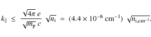
The corresponding condition on the positron kinetic energy, Eq. (8), becomes
![\begin{displaymath}
\ensuremath{E_{k}}\ge (511~{\rm keV}) \
\left[
\sqrt{
1....
...\frac{B_{\rm\mu G}^2}{n_{\rm i,cm^{-3}}}
+ 1
} - 1
\right] .
\end{displaymath}](/articles/aa/full_html/2009/48/aa09830-08/img115.png)
The above expressions were obtained on the assumption that the only ion present in the ISM is H+. To account for the presence of other ions, it suffices, to a good approximation, to replace
The maximum parallel wavenumber,
![]() ,
and the minimum
kinetic energy,
,
and the minimum
kinetic energy,
![]() ,
given by the right-hand sides of
Eqs. (12) and (13), respectively,
are listed in Table 1 for the different phases of the ISM.
Also listed in Table 1 are the estimated temperature, T,
magnetic field strength, B, hydrogen density,
,
given by the right-hand sides of
Eqs. (12) and (13), respectively,
are listed in Table 1 for the different phases of the ISM.
Also listed in Table 1 are the estimated temperature, T,
magnetic field strength, B, hydrogen density, ![]() ,
and
ionization fraction,
,
and
ionization fraction,
![]() of the different phases. The values of T,
of the different phases. The values of T, ![]() and
and
![]() are taken from the review paper of
Ferrière (2001).
For B, we adopt the value of
are taken from the review paper of
Ferrière (2001).
For B, we adopt the value of
![]() inferred from rotation
measure studies (e.g. Ohno & Shibata 1993; Rand & Kulkarni 1989) for the
warm phases, the value of
inferred from rotation
measure studies (e.g. Ohno & Shibata 1993; Rand & Kulkarni 1989) for the
warm phases, the value of
![]() inferred from Zeeman
splitting measurements (Heiles & Troland 2005) for the cold phase,
the relation
inferred from Zeeman
splitting measurements (Heiles & Troland 2005) for the cold phase,
the relation
![]() normalized to
normalized to
![]() at
at
![]() (Crutcher 1999) for molecular clouds, and the two extreme
values of
(Crutcher 1999) for molecular clouds, and the two extreme
values of
![]() and
and
![]() for the hot phase. The
lower value pertains to the standard scenario in which the hot gas is
generated by stellar winds and supernova explosions, which sweep up
the ambient magnetic field lines and evacuate them from the hot
cavities. The higher value pertains to an alternative scenario in
which large-scale highly turbulent MHD fluctuations produce magnetic
fields above equipartition with the local thermal pressure
(Bykov 2001; Parizot et al. 2004b; and references therein).
for the hot phase. The
lower value pertains to the standard scenario in which the hot gas is
generated by stellar winds and supernova explosions, which sweep up
the ambient magnetic field lines and evacuate them from the hot
cavities. The higher value pertains to an alternative scenario in
which large-scale highly turbulent MHD fluctuations produce magnetic
fields above equipartition with the local thermal pressure
(Bykov 2001; Parizot et al. 2004b; and references therein).
From Table 1, it emerges that the maximum parallel
wavenumber of Alfvén waves is typically a few
![]() ,
close to the largest wavenumber,
,
close to the largest wavenumber,
![]() ,
of the electron density power spectrum
inferred from interstellar scintillation (Armstrong et al. 1995).
Furthermore, the minimum kinetic energy required for positrons to
interact resonantly with Alfvén waves varies from a few keV (in the
warm ionized medium) to a few hundreds of keV (in regions with large
Alfvén speeds, namely, in molecular clouds and possibly in the warm
neutral and hot ionized media). For comparison, positrons produced by
radioactive decay are injected into the ISM with typical kinetic
energies
,
of the electron density power spectrum
inferred from interstellar scintillation (Armstrong et al. 1995).
Furthermore, the minimum kinetic energy required for positrons to
interact resonantly with Alfvén waves varies from a few keV (in the
warm ionized medium) to a few hundreds of keV (in regions with large
Alfvén speeds, namely, in molecular clouds and possibly in the warm
neutral and hot ionized media). For comparison, positrons produced by
radioactive decay are injected into the ISM with typical kinetic
energies ![]() 1 MeV. This means that positrons from radioactive
decay can interact resonantly with Alfvén waves only over a
restricted energy range. This range is particularly narrow in regions
with large Alfvén speeds, such as molecular clouds (where
1 MeV. This means that positrons from radioactive
decay can interact resonantly with Alfvén waves only over a
restricted energy range. This range is particularly narrow in regions
with large Alfvén speeds, such as molecular clouds (where
![]() ); it can even vanish in the hot phase if
the magnetic field is as strong as
); it can even vanish in the hot phase if
the magnetic field is as strong as
![]() (implying
(implying
![]() ). In contrast, the resonant range
extends over at least two orders of magnitude in the warm ionized
medium, where the ion density is highest (and
). In contrast, the resonant range
extends over at least two orders of magnitude in the warm ionized
medium, where the ion density is highest (and
![]() ). The reason why resonant interactions with
Alfvén waves are no longer possible below
). The reason why resonant interactions with
Alfvén waves are no longer possible below
![]() is
because the Larmor radius has become smaller than the smallest
possible scale of existing Alfvén waves.
is
because the Larmor radius has become smaller than the smallest
possible scale of existing Alfvén waves.
Fast magnetosonic waves
The numerical expressions and values of the wavenumber and kinetic
energy thresholds can be obtained in the same manner as for Alfvén
waves, with the two following differences: First, the wavenumber
threshold (Eq. (9)) applies to the total
wavenumber, as opposed to the parallel wavenumber. Second, the speed
entering the expressions of the thresholds is the phase speed of the
fast mode for parallel propagation,
![]() ,
as opposed to the
Alfvén speed,
,
as opposed to the
Alfvén speed, ![]() .
In practice, however, the second
difference is only formal, except in the hot low-B phase. Indeed,
.
In practice, however, the second
difference is only formal, except in the hot low-B phase. Indeed,
![]() ,
and
,
and
![]() in all the ISM phases, except in
the hot low-B phase, where
in all the ISM phases, except in
the hot low-B phase, where
![]() .
In consequence, the values of the
maximum wavenumber,
.
In consequence, the values of the
maximum wavenumber,
![]() ,
and the minimum kinetic energy,
,
and the minimum kinetic energy,
![]() ,
are those listed in Table 1, except in the
hot low-B phase, for which Eqs. (9) and
(11) lead to
,
are those listed in Table 1, except in the
hot low-B phase, for which Eqs. (9) and
(11) lead to
![]() and
and
![]() ,
respectively. The latter value is roughly an order of magnitude
larger than for Alfvén waves, which significantly narrows down the
energy range over which positrons from radioactive decay can interact
resonantly with fast magnetosonic waves.
,
respectively. The latter value is roughly an order of magnitude
larger than for Alfvén waves, which significantly narrows down the
energy range over which positrons from radioactive decay can interact
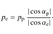
resonantly with fast magnetosonic waves.
The Cherenkov resonance (for ![]() )
occurs when
)
occurs when
![]() ,
i.e., at a wave propagation angle
,
i.e., at a wave propagation angle
![]() such that
such that
![]() ,
independent of the wavenumber. Since
,
independent of the wavenumber. Since
![]() never departs from the fast magnetosonic speed,
never departs from the fast magnetosonic speed,
![]() ,
by more than a factor
,
by more than a factor ![]() ,
this expression is
approximately equivalent to
,
this expression is
approximately equivalent to
![]() .
The Cherenkov resonance requires that the wave at
propagation angle
.
The Cherenkov resonance requires that the wave at
propagation angle
![]() exist and not be damped by a
collisional or collisionless process (see next subsections).
exist and not be damped by a
collisional or collisionless process (see next subsections).
Let us re-emphasize that the above results should be considered only as rough estimates. As we will now see, both Alfvén and fast magnetosonic waves are subject to various damping processes in the ISM.
2.2 MHD wave cascades
2.2.1 Energy transfer timescales
We consider both Alfvén waves and fast magnetosonic waves as parts
of turbulent cascades. The main sources of turbulence able to
counterbalance the dissipation mechanisms expected in the ISM are
the magnetorotational instability driven by the differential rotation
of the Galaxy and the explosion of supernovae (Mac Low & Klessen 2004).
Both mechanisms release energy at large scales. In the rest of the
paper, we adopt
![]() pc for the injection scale.
This does not preclude the possibility of injecting magnetic
fluctuations at smaller scales; an issue discussed in Sect. 2.4.
pc for the injection scale.
This does not preclude the possibility of injecting magnetic
fluctuations at smaller scales; an issue discussed in Sect. 2.4.
Alfvén wave cascade
The most recent developments in MHD turbulence theory explain the
energy cascade towards smaller scales by the distortion of oppositely
travelling Alfvén wave packets
(e.g., Lithwick & Goldreich 2001). The kinematics of the
interactions produce a highly anisotropic cascade, which
redistributes most of the energy in the perpendicular
scales![]() .
We will return to this important question in Sect. 2.3.
.
We will return to this important question in Sect. 2.3.
The transfer time of the Alfvén wave cascade,
![]() ,
corresponds to the wave packet crossing time along the mean magnetic
field:
,
corresponds to the wave packet crossing time along the mean magnetic
field:

For reference, when
where n is the relevant number density (in a fully ionized medium,
Fast magnetosonic wave cascade
The transfer time of the fast magnetosonic wave cascade,
![]() ,
can be written as
,
can be written as
where
with the density n defined as for the Alfvén wave cascade.
For both Alfvén and fast magnetosonic waves, the dominant damping
process depends on the wavelength (or inverse wavenumber) compared to
the proton collisional mean free-path,
where
and
(Braginskii 1965). Waves with
As we will see below, in all the cases considered here,
![]() ,
which means that both turbulent cascades start in
the collisional range. The wave energy is then transferred to smaller
scales up to the point where the wave damping rate,
,
which means that both turbulent cascades start in
the collisional range. The wave energy is then transferred to smaller
scales up to the point where the wave damping rate, ![]() ,
becomes
equal to the transfer rate. In other words, the turbulent cascades
are cut off at a wavenumber
,
becomes
equal to the transfer rate. In other words, the turbulent cascades
are cut off at a wavenumber
![]() such that
such that
for the Alfvén cascade and
for the fast magnetosonic cascade. If the collisional damping rate,
2.2.2 Damping and cutoff
In this section, we summarize the investigation presented in Appendix A on the dominant damping processes of the Alfvén and fast magnetosonic wave cascades in the different ISM phases.
In the mostly neutral, atomic and molecular phases of the ISM,
the Alfvén and fast magnetosonic wave cascades are, regardless of
their origin, both cut off by ion-neutral collisions at scales larger
than the proton mean free-path,
![]() ,
i.e.,
in the collisional regime - and thus at scales considerably
larger
than the Larmor radii of interstellar positrons.
In consequence, positrons will find no Alfvén or fast magnetosonic
waves from an MHD cascade to resonantly interact with (see also
Higdon et al. 2009).
,
i.e.,
in the collisional regime - and thus at scales considerably
larger
than the Larmor radii of interstellar positrons.
In consequence, positrons will find no Alfvén or fast magnetosonic
waves from an MHD cascade to resonantly interact with (see also
Higdon et al. 2009).
The situation is completely different in the ionized phases of the
ISM. There, the Alfvén wave cascade develops with insignificant
(collisional) damping down to
![]() .
It then enters the
collisionless range, where it
is eventually cut off by linear Landau damping around the proton
inertial length. Thus, the extended inertial range of the Alfvén
wave
cascade leaves some room for possible resonant interactions with
positrons. The fast magnetosonic wave cascade, for its part, suffers
strong collisional (viscous) damping. In the warm ionized phase, this
damping is sufficient to destroy the cascade (with the possible
exception of quasi-parallel waves) before it enters the collisionless
range. In the hot ionized phase, the cascade manages to reach the
collisionless range, but it is then quickly destroyed by linear
Landau damping (again with the possible exception of quasi-parallel
waves).
Altogether, no fast magnetosonic waves from an MHD cascade have
sufficiently small scales to come into resonant interactions with
positrons.
.
It then enters the
collisionless range, where it
is eventually cut off by linear Landau damping around the proton
inertial length. Thus, the extended inertial range of the Alfvén
wave
cascade leaves some room for possible resonant interactions with
positrons. The fast magnetosonic wave cascade, for its part, suffers
strong collisional (viscous) damping. In the warm ionized phase, this
damping is sufficient to destroy the cascade (with the possible
exception of quasi-parallel waves) before it enters the collisionless
range. In the hot ionized phase, the cascade manages to reach the
collisionless range, but it is then quickly destroyed by linear
Landau damping (again with the possible exception of quasi-parallel
waves).
Altogether, no fast magnetosonic waves from an MHD cascade have
sufficiently small scales to come into resonant interactions with
positrons.
2.3 Positron interactions with MHD wave cascades
Our previous discussion indicates that the MHD cascades are truncated
at scales several orders of magnitude larger than the Larmor radii
of positrons produced by radioactive decay or as cosmic rays, except
in the hot and warm ionized phases of the ISM. In these phases, Alfvén
wave turbulence is expected to cascade nearly undamped down to scales
close to the Larmor radius of MeV positrons. However, as we now argue, this
does not necessarily mean that short-wavelength Alfvén waves will resonantly
interact with MeV positrons. Indeed, magnetic fluctuations are probably highly
anisotropic at small scales, in the sense that turbulent eddies are strongly
elongated along the mean magnetic field, or, in mathematical terms,
![]() (Goldreich & Sridhar 1995; Yan & Lazarian 2004).
Because of the important anisotropy of magnetic fluctuations, which
increases towards smaller scales, scattering off Alfvén waves appears
questionable. The elongated irregularities associated with anisotropic
turbulence average out over a particle gyration (Chandran 2000).
If some Alfvén waves are present at scales
(Goldreich & Sridhar 1995; Yan & Lazarian 2004).
Because of the important anisotropy of magnetic fluctuations, which
increases towards smaller scales, scattering off Alfvén waves appears
questionable. The elongated irregularities associated with anisotropic
turbulence average out over a particle gyration (Chandran 2000).
If some Alfvén waves are present at scales
![]() ,
the scattering frequency is reduced by more than 20 orders of magnitude
compared to the situation with isotropic turbulence
(see, for instance, Yan & Lazarian 2002). Slab turbulence gives the
same order of estimates (Yan & Lazarian 2004). In consequence, scattering
off Alfvén wave turbulence should be extremely inefficient at confining
positrons in the ionized phases of the ISM. In this view, the diffusion models
for positron transport adopted in a series of recent papers by
Cheng et al. (2006); Jean et al. (2006); Parizot et al. (2005), using diffusion coefficients
derived from quasi-linear theory, overestimate the confinement by plasma waves.
,
the scattering frequency is reduced by more than 20 orders of magnitude
compared to the situation with isotropic turbulence
(see, for instance, Yan & Lazarian 2002). Slab turbulence gives the
same order of estimates (Yan & Lazarian 2004). In consequence, scattering
off Alfvén wave turbulence should be extremely inefficient at confining
positrons in the ionized phases of the ISM. In this view, the diffusion models
for positron transport adopted in a series of recent papers by
Cheng et al. (2006); Jean et al. (2006); Parizot et al. (2005), using diffusion coefficients
derived from quasi-linear theory, overestimate the confinement by plasma waves.
To circumvent this problem, Yan & Lazarian (2004) reconsidered scattering
off fast magnetosonic waves, emphasizing the isotropy of the
fast wave cascade. As we saw earlier, in the hot and warm ionized phases,
fast waves decay away at scales much larger than the Larmor radii
of positrons from radioactivity, except possibly at quasi-parallel
propagation. If propagation angles are not or only weakly randomized
by wave-wave interactions or by chaotic divergence of magnetic field lines,
quasi-parallel waves may survive down to much smaller scales.
In that case, they may be involved either in gyroresonance or in
Cherenkov resonance, also known as transit-time damping (TTD) resonance, with
positrons. As explained at the end of Sect. 2.1, Cherenkov resonance
occurs at propagation angles
![]() such that
such that
![]() ,
independent of the wavelength. But we know that only those fast waves with
,
independent of the wavelength. But we know that only those fast waves with
![]() have a chance to escape heavy damping. From this, we conclude that only positrons with pitch angles
satisfying
have a chance to escape heavy damping. From this, we conclude that only positrons with pitch angles
satisfying
![]() have a chance to
experience TTD resonance. At precisely
have a chance to
experience TTD resonance. At precisely
![]() ,
the TTD mechanism
vanishes, but its rate rises rapidly as
,
the TTD mechanism
vanishes, but its rate rises rapidly as
![]() increases
above
increases
above
![]() (Schlickeiser & Miller 1998).
Ultimately, positrons produced by radioactive decay are unlikely to
efficiently interact with MHD waves from a direct cascade
generated at large scales. Such positron-wave interactions appear to be
completely ruled out in the neutral phases of the ISM. In the ionized phases, they could
potentially take place, but only under very restrictive conditions, including quasi-parallel
fast waves (
(Schlickeiser & Miller 1998).
Ultimately, positrons produced by radioactive decay are unlikely to
efficiently interact with MHD waves from a direct cascade
generated at large scales. Such positron-wave interactions appear to be
completely ruled out in the neutral phases of the ISM. In the ionized phases, they could
potentially take place, but only under very restrictive conditions, including quasi-parallel
fast waves (
![]() )
and nearly perpendicular positron
motion (
)
and nearly perpendicular positron
motion (
![]() ).
).
Of course, an additional local injection of MHD waves at much smaller scales could participate in the confinement of positrons. Some aspects of this possibility will be discussed in Sect. 2.5.
2.4 Wave injection through plasma instabilities
As we saw in the previous subsection, MHD waves injected at large scales
into an MHD cascade are generally unable to efficiently interact with
positrons from radioactive decay. However, MHD waves can be injected
into the ISM by a variety of fluid or kinetic instabilities, which
involve changes over the whole or a fraction of the velocity distribution
of some particle population. These waves can be injected at scales
![]() ,
possibly directly into the collisionless regime.
Each case requires a dedicated investigation of the wave damping process.
The scale of the turbulence injection is a key parameter controlling
the interaction between MHD waves and positrons. First,
,
possibly directly into the collisionless regime.
Each case requires a dedicated investigation of the wave damping process.
The scale of the turbulence injection is a key parameter controlling
the interaction between MHD waves and positrons. First,
![]() controls the anisotropy of the Alfvén wave cascade at the scale of
the Larmor radius of positrons. Second, it also controls the cutoff
wavenumber and the propagation angle of the fast magnetosonic cascade
(see Eq. (A.18)). In this subsection, we
focus on some particular aspects of one type of kinetic instability.
controls the anisotropy of the Alfvén wave cascade at the scale of
the Larmor radius of positrons. Second, it also controls the cutoff
wavenumber and the propagation angle of the fast magnetosonic cascade
(see Eq. (A.18)). In this subsection, we
focus on some particular aspects of one type of kinetic instability.
One of the most widely studied kinetic instabilities is triggered by the streaming of cosmic rays in the ISM, with a bulk velocity larger than a few times the local Alfvén speed (Wentzel 1974; Skilling 1975). The streaming instability is expected to develop mainly in the intercloud medium. Cosmic-ray streaming compensates for the sink in the low-energy cosmic-ray population due to strong ionization losses inside molecular clouds. Low-energy cosmic rays scatter off their self-generated waves, and are, therefore, excluded from molecular clouds (Dogel & Sharov 1985; Skilling & Strong 1976; Cesarsky & Volk 1978; Lerche 1967). This scenario was adapted to the transport of cosmic-ray electrons by Morfill (1982). The streaming instability and other kinds of kinetic instabilities recently received new attention in the context of cosmic-ray diffusion in anisotropic MHD turbulence (Farmer & Goldreich 2004; Lazarian & Beresnyak 2006).
Here, we restrict our discussion to the sole streaming instability.
The waves are generated at scales
![]() close to the
gyroradii of low-energy cosmic rays, so that
close to the
gyroradii of low-energy cosmic rays, so that
![]() .
If the waves generated by cosmic rays are to serve as scattering
agents for low-energy positrons, then the Landau-synchrotron resonance
condition has to be fulfilled by both species, i.e., by virtue of
Eq. (3):
.
If the waves generated by cosmic rays are to serve as scattering
agents for low-energy positrons, then the Landau-synchrotron resonance
condition has to be fulfilled by both species, i.e., by virtue of
Eq. (3):
Equation (19) implies that the wave-generating cosmic rays and the scattered positrons must have comparable momenta, unless the ratio of angular factors is very different from unity. Now, the wave-generating cosmic rays have typical momenta in the range
Higdon et al. (2009) proposed an alternative mechanism whereby positrons scatter off their own self-generated waves. The growth rate of such an instability is proportional to the density of resonant particles. The positron density depends strongly on their position with respect to the sources. Higdon et al. (2009) argued that whistler waves are heavily damped in the neutral phases of the ISM, but the streaming instability may also operate close to the sources (for instance close to supernova remnants; see Ptuskin et al. 2008) or above the Galactic disk where the ionization fraction can be close to unity. A complete estimation of this process deserves a detailed investigation and will be considered in a forthcoming paper.
2.5 Positron transport in dissipated turbulence and re-acceleration
In the solar wind, MeV positrons can also interact with perturbations
that fall into the dissipative range of the turbulence, above the
steepening observed at a fraction of the proton gyrofrequency at
wavenumbers
![]() .
It has been proposed that low-frequency
non-resonant magnetosonic waves can dominate the propagation of
sub-MeV particles if magnetosonic waves are present in the solar wind
(Toptygin 1985; Ragot 2006).
Ragot (1999) suggested that non-resonant fast magnetosonic
waves can produce efficient angular scattering through pitch angles
.
It has been proposed that low-frequency
non-resonant magnetosonic waves can dominate the propagation of
sub-MeV particles if magnetosonic waves are present in the solar wind
(Toptygin 1985; Ragot 2006).
Ragot (1999) suggested that non-resonant fast magnetosonic
waves can produce efficient angular scattering through pitch angles
![]() and thus govern the particle mean
free-path at energies
and thus govern the particle mean
free-path at energies ![]() 1 MeV. This result could be applied
to the stellospheres of massive stars (about a few parsecs)
and to larger regions of the ISM (see discussion in Higdon et al. (2009),
though in a different perspective).
1 MeV. This result could be applied
to the stellospheres of massive stars (about a few parsecs)
and to larger regions of the ISM (see discussion in Higdon et al. (2009),
though in a different perspective).
The electric component of the waves induces a variation
in particle energy. The average effect of such interactions
leads to a stochastic energy gain, also known as second-order
Fermi acceleration.
Particle stochastic acceleration (also referred to as re-acceleration)
is important
if the re-acceleration time is shorter than the energy loss time,
i.e., if
![]() .
The re-acceleration time is related to the momentum diffusion coefficient
Dp through
.
The re-acceleration time is related to the momentum diffusion coefficient
Dp through
![]() (here, we consider
only pitch-angle averaged quantities).
It can also be expressed in terms of the particle angular diffusion
frequency
(here, we consider
only pitch-angle averaged quantities).
It can also be expressed in terms of the particle angular diffusion
frequency
![]() as
as
![]() .
Then the above timescale ordering is equivalent to
.
Then the above timescale ordering is equivalent to
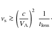
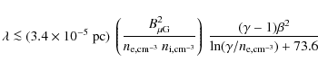
Particles with energies
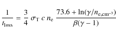
|
(21) |
in an ionized medium and
![\begin{displaymath}\frac{1}{t_{\rm loss}}
= \frac{3}{4} ~ \sigma_{\rm T} ~ c ~ n...
...left[ (\gamma - 1) (\gamma^2 - 1) \right]}{\beta
(\gamma -1)}
\end{displaymath}](/articles/aa/full_html/2009/48/aa09830-08/img202.png)
|
(22) |
in a neutral medium, where
in an ionized medium and
![$\displaystyle \times \frac{(\gamma - 1) \beta^2}{\ln\left[ (\gamma - 1) (\gamma^2 - 1)
\right]+20.5}$](/articles/aa/full_html/2009/48/aa09830-08/img210.png)
in a neutral medium. This implies that if, in a particular medium, the angular diffusion frequency is high enough, particles are reaccelerated. In that case, a solution can be obtained with the help of a diffusion-convection equation. This type of investigation is beyond the scope of the current paper and is postponed to a future work. However, the above discussion already calls some of the results derived by Higdon et al. (2009) into question, as these authors ignored re-acceleration in their analysis. What emerges from the above discussion is that re-acceleration can be important, especially in low-density ionized phases. More specifically, if we introduce the parameter values proposed by Higdon et al. (2009) for the Galactic interstellar bulge (see their Table 1), we find that positron re-acceleration is important in the very hot phase of the inner bulge, and probably in the hot phase of the middle and outer bulge.
3 Effects of collisions with gas particles
In this section, we examine the case when the trajectories of positrons in the ISM is only driven by their collisions with gas particles while they propagate along a steady state magnetic field line, without considering interactions with MHD waves, an aspect usually overlooked by the previous analysis. During these collisions, high-energy positrons not only lose energy, but they also undergo pitch angle scattering. The scattering of kinematic parameters of positrons reduces the maximum distance they can travel along a straight line in the ISM. In Sect. 3.1, we review and describe the interaction processes between positrons and interstellar matter. In Sect. 3.2, we describe the methods used to calculate positron propagation in this so-called ``collisional regime'', and in Sect. 3.3, we present the detailed results of our computations for 1 MeV positrons. The main results obtained for positrons with initial kinetic energies ranging from 1 keV to 10 MeV in typical ISM phases and the case of propagation in a turbulent magnetic field are described in Sect. 3.4.
3.1 Positron interactions with interstellar matter
In the absence of collisions, positrons move along magnetic field lines in helical trajectories. When positrons interact with gas particles, they can either gain or lose energy in elastic and inelastic scattering or even annihilate with free or bound electrons. The energy and pitch angle variations resulting from the interaction depend on the energy of the incident positron and on the velocity and nature of the target particle.
The positrons that we are studying spend most of their lifetime travelling at high energy, with a kinetic energy greater than the thermal energy of target particles in the ISM. Consequently, we do not account for the propagation of positrons at thermal energy, but postpone the discussion of this case to Sect. 3.4.
Interactions of positrons with the ionized component of the
interstellar gas and, at high energy (![]() MeV),
with the magnetic field (synchrotron radiation) and
the interstellar radiation field (inverse Compton scattering)
are generally considered as continuous processes.
They are referred to as continuous energy-loss processes
and are presented in Sect. 3.1.1. In a mostly
neutral gas, positrons lose a larger fraction of their energy
when they excite or ionize atoms or molecules.
Such interactions, which result in a quantified variation
of the positron energy, are described in Sect. 3.1.2.
MeV),
with the magnetic field (synchrotron radiation) and
the interstellar radiation field (inverse Compton scattering)
are generally considered as continuous processes.
They are referred to as continuous energy-loss processes
and are presented in Sect. 3.1.1. In a mostly
neutral gas, positrons lose a larger fraction of their energy
when they excite or ionize atoms or molecules.
Such interactions, which result in a quantified variation
of the positron energy, are described in Sect. 3.1.2.
3.1.1 Continuous energy-loss processes
Figure 1 shows the energy loss rates of positrons as
functions of their energy in a fully ionized plasma
with temperature
![]() .
The energy loss rates by
synchrotron radiation and inverse Compton scattering are
derived from Blumenthal & Gould (1970). They are proportional to
the magnetic-field and photon energy densities, respectively.
The energy loss rate by bremsstrahlung is calculated using the
approximation presented in Ginzburg (1979). The energy
loss rate due to Coulomb collisions (free-free) is calculated using
the Bhabha cross-section as described in Asano et al. (2007).
.
The energy loss rates by
synchrotron radiation and inverse Compton scattering are
derived from Blumenthal & Gould (1970). They are proportional to
the magnetic-field and photon energy densities, respectively.
The energy loss rate by bremsstrahlung is calculated using the
approximation presented in Ginzburg (1979). The energy
loss rate due to Coulomb collisions (free-free) is calculated using
the Bhabha cross-section as described in Asano et al. (2007).
![\begin{figure}
\par\includegraphics*[scale=1]{09830fg1.eps}
\end{figure}](/articles/aa/full_html/2009/48/aa09830-08/img216.png)
|
Figure 1:
Energy-loss rates of positrons in a 8000 K plasma with
number densities
|
| Open with DEXTER | |
In a fully ionized plasma, Coulomb collisions represent the
dominant loss process for positrons with ![]() 100 MeV.
Since the energy loss rates by synchrotron radiation and inverse
Compton scattering depend on the magnetic-field and photon energy
densities, they vary with the location of positrons in our Galaxy.
It is expected that inverse Compton losses become
dominant in zones close to stellar clusters.
However, we are interested in positrons
with kinetic energy
100 MeV.
Since the energy loss rates by synchrotron radiation and inverse
Compton scattering depend on the magnetic-field and photon energy
densities, they vary with the location of positrons in our Galaxy.
It is expected that inverse Compton losses become
dominant in zones close to stellar clusters.
However, we are interested in positrons
with kinetic energy ![]() 10 MeV and, therefore, we
may neglect synchrotron losses as long as
10 MeV and, therefore, we
may neglect synchrotron losses as long as ![]() mG.
mG.
The average scattering angle induced by Coulomb collisions
occurring over a time interval ![]() is estimated through the
relation
is estimated through the
relation
where
where n is the number density of target particles,
While the energy loss rate from e+p collisions is negligible compared to that from e+e- collisions, their deviation rates are equivalent. We checked that the resulting deviation rates are in agreement with those derived at low energy using the formalism of Huba (2006).
3.1.2 Annihilation and interactions with atoms and molecules
In a neutral medium, high-energy positrons lose energy mainly by ionizing and exciting atoms and molecules, or they annihilate directly with bound electrons, the elastic scattering process being negligible at these energies (see Charlton & Humberston 2000 and Wallyn et al. 1994). Such interactions occur at random while positrons propagate in the ISM. Therefore, we will determine the kind of interaction and calculate the variation of the kinematic parameters with a Monte-Carlo method that incorporates the corresponding cross sections.
The ionization and excitation cross sections as well as the differential cross sections as functions of the energy lost by positrons in ionizing collisions were calculated by Gryzinski (1965c,a,b). The cross section of annihilation in flight of positrons with bound electrons is equal to that of annihilation with free electrons, since the binding energy of electrons is negligible with respect to the kinetic energy of the positrons under study. We use the cross section of annihilation with free electrons presented in Guessoum et al. (2005, and references therein).
In the Monte-Carlo simulations, the energy lost by a positron when it ionizes an atom/molecule is chosen randomly according to its differential cross section. The energy lost by a positron when it excites an atom/molecule is derived from the energies of the atomic levels involved in the interaction. Once the energy lost by ionization or excitation is known, the scattering angle of the positron is calculated with the kinematics of the interaction, assuming that the atoms/molecules stay at rest and assuming azimuthal symmetry.
3.2 Simulations of the collisional transport
Our Monte-Carlo simulations are based on the methods presented in Bussard et al. (1979) and Guessoum et al. (2005). However, we add the calculation of the trajectories of positrons while they propagate along magnetic field lines and include additional steps to account for the scattering of positrons by collisions.
At the initial time (k=0), positrons are located
at
(x,y,z,t)=(0,0,0,0) in a
frame such that the magnetic field ![]() is directed along
the z axis. The initial kinetic energy of positrons is E0.
The direction of their initial velocity
is directed along
the z axis. The initial kinetic energy of positrons is E0.
The direction of their initial velocity
![]() ,
which is defined by their initial pitch angle
,
which is defined by their initial pitch angle
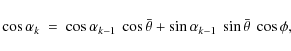
![]() and their
initial phase
and their
initial phase ![]() (see Fig. 2), is chosen randomly
according to an isotropic velocity distribution in the entire space.
(see Fig. 2), is chosen randomly
according to an isotropic velocity distribution in the entire space.
![\begin{figure}
\par\includegraphics*[scale=0.93,clip]{09830fg2.eps}
\end{figure}](/articles/aa/full_html/2009/48/aa09830-08/img235.png)
|
Figure 2:
Kinematic parameters of the scattering in the laboratory frame. The magnetic field |
| Open with DEXTER | |
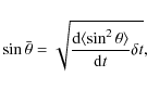
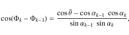
We proceed through successive iterations. At step k, the resulting
pitch angle (
![]() )
and phase (
)
and phase (![]() )
are given by
)
are given by
|
(28) |
where the azimuthal scattering angle
![\begin{displaymath}{R}=\exp\left[-\int_{E_{k-1}}^{E_{k}}\frac{\upsilon \ \sum\li...
...,j}n_j \
\sigma_{i,j}(E)}{{\rm d}E/{\rm d}t}~{\rm d}E\right],
\end{displaymath}](/articles/aa/full_html/2009/48/aa09830-08/img239.png)
|
(29) |
where R is a random number uniformly distributed between 0 and 1,
|
(30) |
The energy lost and the scattering angle induced by collisions are derived using the methods presented in Sect. 3.1.2.
The increment in time between two iterations, ![]() ,
is equal to
a scattering time
,
is equal to
a scattering time
![]() defined as
defined as
|
(31) |
with
Between two steps and/or two interactions, positrons propagate
in a regular helical trajectory along magnetic field lines
with a gyroradius
![]() (defined
in Sect. 2.1). The positron position after each step
is therefore calculated analytically.
(defined
in Sect. 2.1). The positron position after each step
is therefore calculated analytically.
The above procedure is repeated until positrons annihilate or their kinetic energy falls below 100 eV, since the distance traveled below this energy becomes negligible. To estimate the spatial distribution of positrons and their lifetime, we read out the positron location and slowing-down time at the end of the track. To save CPU time while obtaining sufficiently accurate results, Monte-Carlo simulations are performed with a number of positrons ranging from 5000 to 20 000.
To validate our code, we performed several tests for positrons with E0 < 10 MeV released in different media and we compared the results of our simulations with previous work. The fractions of positrons annihilating in flight with free or bound electrons are in agreement with the results presented by Beacom & Yüksel (2006) and Sizun et al. (2006). At low energy (E0 < 1 keV), the fractions of positronium formed in flight by charge exchange with atoms and molecules in different media are identical to those obtained by Guessoum et al. (2005). Once positrons are thermalized, their propagation behaves as classical diffusion. The distance they travel then is negligible compared to the distance traveled in the slowing-down regime, except in the hot medium (see Sect. 3.4).
3.3 Results of the simulations for 1 MeV positrons
This section presents, as an illustrative example, the
detailed results of simulations obtained for positrons with
initial kinetic energy E0 = 1 MeV. For this first set of
simulations, we chose the warm medium, whose temperature is
intermediate between those of the cold and hot media. The warm medium
is also the most appropriate medium to study the impact of the
ionization fraction, which covers the whole possible range between 0
and 1. We assumed the magnetic field to be uniform, with a strength
![]() .
.
![\begin{figure}
\par\includegraphics*[scale=0.33,clip]{09830fg3.eps}
\end{figure}](/articles/aa/full_html/2009/48/aa09830-08/img248.png)
|
Figure 3:
Spatial distributions of positrons along field lines at the end of their slowing-down period in a warm medium (T = 8000 K and
|
| Open with DEXTER | |
Since the energy loss rates and the frequency of inelastic interactions
are proportional to the target density, for given
abundances and a given ionization fraction, the distance traveled by positrons
scales as the inverse of the total density.
Therefore, we performed simulations for
![]() ,
with
,
with
![]() the total
number density of hydrogen nuclei. Preliminary tests
of our simulations indicate that the presence of
ionized or neutral helium with an abundance ratio
the total
number density of hydrogen nuclei. Preliminary tests
of our simulations indicate that the presence of
ionized or neutral helium with an abundance ratio
![]() does not strongly affect positron propagation (differences less
than 10%). We also neglected molecular hydrogen, except in the MM
where
does not strongly affect positron propagation (differences less
than 10%). We also neglected molecular hydrogen, except in the MM
where ![]() molecules are the dominant species.
molecules are the dominant species.
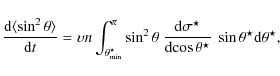
Figure 3 shows the spatial distributions of positrons
along the magnetic field direction (z), as extracted from our simulations,
once they reach E = 100 eV. Positrons are initially ``injected'' at
(x,y,z)=(0,0,0) with a pitch angle chosen randomly according
to an isotropic velocity distribution in the entire space.
The temperature is 8000 K and the
ionization fraction ranges from 0 to 1.
The field-aligned distributions are nearly uniform out to the
maximum distance traveled along field lines,
![]() (obtained
when the pitch angle is and remains equal to 0). This means that the
pitch angle does not change significantly over most of the
slowing-down period of positrons. If the pitch angle remained
strictly constant, the distance traveled along field lines
would be equal to
(obtained
when the pitch angle is and remains equal to 0). This means that the
pitch angle does not change significantly over most of the
slowing-down period of positrons. If the pitch angle remained
strictly constant, the distance traveled along field lines
would be equal to
![]() .
Since positrons are initially emitted isotropically,
.
Since positrons are initially emitted isotropically,
![]() is uniformly distributed between -1 and 1, so that the
field-aligned distributions of positrons at the end of their
slowing-down period would be uniform. In reality, the slight pitch
angle scattering induced by collisions produces a slight scattering of their
final field-aligned positions and, therefore, smoothes out
the edge of the otherwise uniform distributions.
The maximum distance
is uniformly distributed between -1 and 1, so that the
field-aligned distributions of positrons at the end of their
slowing-down period would be uniform. In reality, the slight pitch
angle scattering induced by collisions produces a slight scattering of their
final field-aligned positions and, therefore, smoothes out
the edge of the otherwise uniform distributions.
The maximum distance
![]() is obtained by integrating over
energy the ratio of the positron velocity to the energy loss rate.
In the present case, the energy loss rate is the sum of the
contributions from Coulomb collisions (see Sect. 3.1.1)
and inelastic interactions (ionization and excitation) with atoms
and molecules. The latter contributions are evaluated using the
Bethe-Bloch formula (Ginzburg 1979).
is obtained by integrating over
energy the ratio of the positron velocity to the energy loss rate.
In the present case, the energy loss rate is the sum of the
contributions from Coulomb collisions (see Sect. 3.1.1)
and inelastic interactions (ionization and excitation) with atoms
and molecules. The latter contributions are evaluated using the
Bethe-Bloch formula (Ginzburg 1979).
The extent of the spatial distributions in the directions perpendicular to the magnetic field is a few times the Larmor radius, i.e., negligible with respect to the extent of the field-aligned distributions. We characterize the extent of the field-aligned distributions presented in Fig. 3 by their full width at half maximum (FWHM//). Its uncertainty is calculated with a bootstrap method taking into account the uncertainty in the number of positrons (Poisson statistics) in each spatial bin.
The extent of the field-aligned distributions increases naturally with
decreasing ionization fraction (see Fig. 3), since
the energy losses through Coulomb collisions dominate over the losses
due to inelastic interactions (ionization and excitation) with
neutrals. Depending on the ionization fraction, the half FWHM//
is 15% to 30% lower than
![]() .
.
3.4 Transport of positrons in the different ISM phases
This section summarizes the results of the simulations for positrons with initial kinetic energies ranging from 1 keV to 10 MeV, in the different ISM phases.
Figure 4 shows the extent (FWHM//) of the field-aligned
distribution of positrons at the end of their slowing-down time (i.e.,
when they reach 100 eV), as a function of their initial kinetic energy
in the different ISM phases. As in Sect. 3.3 , the hydrogen
density is arbitrarily set to
![]() ,
and the ionization
fraction is 0, 0.001, 0.1, 0.9 and 1 in the MM, CM, WNM, WIM and HIM,
respectively.
The extents presented in Fig. 4 are compared to the extents
that the distributions would have if the positron pitch angles remained
constant, namely, 2
,
and the ionization
fraction is 0, 0.001, 0.1, 0.9 and 1 in the MM, CM, WNM, WIM and HIM,
respectively.
The extents presented in Fig. 4 are compared to the extents
that the distributions would have if the positron pitch angles remained
constant, namely, 2
![]() .
In each ISM phase and for any given initial energy, FWHM// is
similar to, and always slightly less than, 2
.
In each ISM phase and for any given initial energy, FWHM// is
similar to, and always slightly less than, 2
![]() ,
as expected
from the effect of pitch angle scattering.
,
as expected
from the effect of pitch angle scattering.
![\begin{figure}
\par\includegraphics*[scale=0.33,clip]{09830fg4.eps}
\end{figure}](/articles/aa/full_html/2009/48/aa09830-08/img254.png)
|
Figure 4:
FWHM of the field-aligned distributions of at the end of their
slowing-down period, as functions of their initial kinetic energy. The
hydrogen density is arbitrarily set to
|
| Open with DEXTER | |
The above FWHM// extents are given assuming a uniform magnetic field in the z direction. However, field lines in the ISM are perturbed by turbulent motions. As a result, realistic magnetic fields in the ISM consist of a mean (``regular'') component plus a turbulent component, leading to chaotic field lines. The distances traveled by positrons along the uniform field (i.e., along the z axis) are shorter than the total distances traveled along the actual chaotic field lines.
We estimate the effects of the turbulent magnetic field on the distances
traveled by positrons by adding a turbulent component to the uniform
field. This turbulent field
is modelled using the plane wave approximation method presented
by Giacalone & Jokipii (1994). We assume a ratio
![]() .
The fluctuations follow a Kolmogorov spectrum and have a maximum
turbulent scale
.
The fluctuations follow a Kolmogorov spectrum and have a maximum
turbulent scale
![]() 10-100 pc in the hot
and warm phases and
10-100 pc in the hot
and warm phases and
![]() 1-10 pc in
the cold neutral and molecular phases.
These scale lengths correspond to the typical sizes of the respective phases.
Since the Larmor radii of positrons with kinetic energies in the considered
range are extremely small compared to the turbulent scale lengths,
positrons simply propagate along the turbulent field lines.
Under these conditions, the actual coordinates of positrons at the end of their
slowing-down period are obtained by carrying their coordinates along the
uniform field (as calculated in Sect. 3.3) over
to the curvilinear frame of the turbulent field lines. These
coordinates are calculated by
Monte-Carlo simulations, using a large number of randomly chosen turbulent
configurations for a given
1-10 pc in
the cold neutral and molecular phases.
These scale lengths correspond to the typical sizes of the respective phases.
Since the Larmor radii of positrons with kinetic energies in the considered
range are extremely small compared to the turbulent scale lengths,
positrons simply propagate along the turbulent field lines.
Under these conditions, the actual coordinates of positrons at the end of their
slowing-down period are obtained by carrying their coordinates along the
uniform field (as calculated in Sect. 3.3) over
to the curvilinear frame of the turbulent field lines. These
coordinates are calculated by
Monte-Carlo simulations, using a large number of randomly chosen turbulent
configurations for a given
![]() .
Figure 5
shows examples of the positions of positrons at the end of the
slowing-down time, calculated with this method in a WIM with
.
Figure 5
shows examples of the positions of positrons at the end of the
slowing-down time, calculated with this method in a WIM with
![]() = 0.2 cm-3 and
= 0.2 cm-3 and
![]() .
.
![\begin{figure}
\par\includegraphics*[scale=0.33,clip]{09830f5a.eps}\vspace*{2.5m...
...ps}\vspace*{2.5mm}
\includegraphics*[scale=0.33,clip]{09830f5c.eps}
\end{figure}](/articles/aa/full_html/2009/48/aa09830-08/img258.png)
|
Figure 5:
Positions of positrons at the end of their slowing-down time in a WIM
taking into account collisional transport in a turbulent magnetic field
(
|
| Open with DEXTER | |
![\begin{figure}
\par\includegraphics*[scale=0.33,clip]{09830fg6.eps}
\end{figure}](/articles/aa/full_html/2009/48/aa09830-08/img259.png)
|
Figure 6:
Transverse distributions of positrons at the end of their slowing-down period in a WIM, calculated for maximum turbulent scales
|
| Open with DEXTER | |
![\begin{figure}
\par\includegraphics*[scale=0.33,clip]{09830f7a.eps}\vspace*{2.5mm}
\includegraphics*[scale=0.33,clip]{09830f7b.eps}
\end{figure}](/articles/aa/full_html/2009/48/aa09830-08/img260.png)
|
Figure 7: Minimum and maximum extents of the spatial distributions of positrons reaching 100 eV, along ( top) and perpendicular ( bottom) to the uniform magnetic field, taking into account the turbulent behavior of the field lines as well as realistic values for the density in each ISM phase. |
| Open with DEXTER | |
Adding such a turbulent magnetic field in the simulations
reduces the FWHM of the positron field-aligned distributions by a
factor ![]() 0.75 and broadens their transverse (i.e.,
perpendicular to
0.75 and broadens their transverse (i.e.,
perpendicular to
![]() )
distributions
due to the chaotic behavior of field lines. At low energy,
when the distance traveled by positrons is
shorter than the maximum scale of the turbulence,
)
distributions
due to the chaotic behavior of field lines. At low energy,
when the distance traveled by positrons is
shorter than the maximum scale of the turbulence,
![]() (e.g., Fig. 5a), positrons
have a quasi-uniform distribution along any field line that
can be considered, at this scale, as straight and randomly
tilted with respect to
(e.g., Fig. 5a), positrons
have a quasi-uniform distribution along any field line that
can be considered, at this scale, as straight and randomly
tilted with respect to
![]() .
In this case, the
spatial distribution of positrons is nearly
spherically symmetric. At intermediate energy
(e.g., Fig. 5b), positrons have a more collimated
distribution with a transverse dispersion that increases with
distance from the source. At high energy, when the distance
traveled by positrons is large compared to
.
In this case, the
spatial distribution of positrons is nearly
spherically symmetric. At intermediate energy
(e.g., Fig. 5b), positrons have a more collimated
distribution with a transverse dispersion that increases with
distance from the source. At high energy, when the distance
traveled by positrons is large compared to
![]() (e.g., Fig. 5c), the positron distribution is highly
collimated along
(e.g., Fig. 5c), the positron distribution is highly
collimated along
![]() .
.
The shape of the transverse distribution![]() is strongly peaked, as illustrated in
Fig. 6, for positrons with E0 = 1 MeV propagating
in a WIM. The transverse distribution is close to a decaying exponential
function. Its extent increases with
is strongly peaked, as illustrated in
Fig. 6, for positrons with E0 = 1 MeV propagating
in a WIM. The transverse distribution is close to a decaying exponential
function. Its extent increases with
![]() ,
as expected
since a larger scale length leads to larger transverse excursions
of field lines away from the uniform field.
In contrast, the extent of the field-aligned distribution does not
change with
,
as expected
since a larger scale length leads to larger transverse excursions
of field lines away from the uniform field.
In contrast, the extent of the field-aligned distribution does not
change with
![]() ,
because, on average, positrons propagate along
the uniform magnetic field.
,
because, on average, positrons propagate along
the uniform magnetic field.
Due to the cusped shape of the transverse distribution,
FWHM![]() is not necessarily a very meaningful quantity,
as the fraction of
positrons inside FWHM
is not necessarily a very meaningful quantity,
as the fraction of
positrons inside FWHM![]() is low. Moreover, this fraction changes
significantly with
is low. Moreover, this fraction changes
significantly with
![]() (e.g., from
(e.g., from ![]() 1% to
1% to
![]() 9% for the cases presented in Fig. 6) and
with E0 (e.g., from
9% for the cases presented in Fig. 6) and
with E0 (e.g., from ![]() 1% to
1% to ![]() 30% for E0
decreasing from 10 MeV to 1 keV). In contrast, the fraction of positrons
inside the FWHM of the field-aligned distribution ranges from
30% for E0
decreasing from 10 MeV to 1 keV). In contrast, the fraction of positrons
inside the FWHM of the field-aligned distribution ranges from
![]() 80% to
80% to ![]() 95%.
95%.
Consequently, instead of characterizing the spatial extents of the
positron distribution by its FWHM, we will use the field-aligned
length (2z90) and the diameter (2r90) that contain 90% of
the positrons. Figure 7 shows the extents
of the spatial distribution as functions of the initial kinetic
energy of positrons.
The physical conditions (density, ionization fraction, temperature,...)
of the different ISM phases correspond to the extreme values
presented in Table 1. The minimum and maximum spatial
extents are obtained with the maximum and minimum densities and
ionization fractions listed in Table 1 and with the minimum
and maximum
![]() ,
respectively.
,
respectively.
The ratio r90/z90 increases up to ![]() 0.8 with decreasing
energy, confirming that the positron distribution is more isotropic
at low energy. A spherically symmetric distribution would have produced
a ratio r90/
z90 = 1.2.
0.8 with decreasing
energy, confirming that the positron distribution is more isotropic
at low energy. A spherically symmetric distribution would have produced
a ratio r90/
z90 = 1.2.
The results displayed in Fig. 7 show that MeV positrons
travel long distances before reaching 100 eV. Positrons with ![]() 30 keV generally cannot escape molecular clouds (assuming the
smallest size
of molecular clouds is
30 keV generally cannot escape molecular clouds (assuming the
smallest size
of molecular clouds is ![]() 1 pc). On the other hand, positrons with
1 pc). On the other hand, positrons with
![]() 7 keV generally escape the hot medium (assuming the typical size
of hot regions is
7 keV generally escape the hot medium (assuming the typical size
of hot regions is ![]() 200 pc).
200 pc).
So far, we have discussed the distance traveled by positrons over their
slowing-down period, which ends when their kinetic energy falls below 100 eV.
We now consider the distance they travel before annihilating with
electrons. In the neutral phases, low-energy positrons (E<100 eV) annihilate
mostly by forming positroniums through charge exchange processes with
atoms or molecules. The distance they travel before annihilating is negligible
compared to the distance traveled at high energy (see Table 4 of Jean et al.
2006). The situation is different in the ionized phases. There, positrons
quickly thermalize and then annihilate with electrons (via radiative
recombination or direct annihilation). Since the time scale
of annihilation (
![]() )
is inversely proportional to the electron
density, positrons in low-density media may travel a long distance before
annihilating. The rms distance traveled by thermalized positrons along
a uniform magnetic field is
)
is inversely proportional to the electron
density, positrons in low-density media may travel a long distance before
annihilating. The rms distance traveled by thermalized positrons along
a uniform magnetic field is
with the diffusion coefficient
and values of
The rms distance
![]() characterizes the width of the Gaussian
field-aligned distribution of thermalized positrons at the time of
annihilation, when they are initially injected isotropically at z = 0.
Taking into account the turbulent magnetic field, the 3-D spatial distribution
of the sites where positrons annihilate is calculated by carrying their
coordinates along the uniform field over to the curvilinear frame of the
turbulent field lines. We then derive the field-aligned and transverse
extents of this distribution (
characterizes the width of the Gaussian
field-aligned distribution of thermalized positrons at the time of
annihilation, when they are initially injected isotropically at z = 0.
Taking into account the turbulent magnetic field, the 3-D spatial distribution
of the sites where positrons annihilate is calculated by carrying their
coordinates along the uniform field over to the curvilinear frame of the
turbulent field lines. We then derive the field-aligned and transverse
extents of this distribution (
![]() and
and
![]() ,
respectively), defined as the field-aligned length and the diameter that
contain 90% of the annihilating positrons.
In the WIM,
,
respectively), defined as the field-aligned length and the diameter that
contain 90% of the annihilating positrons.
In the WIM,
![]() pc, i.e.,
pc, i.e.,
![]() .
In the HIM,
.
In the HIM,
![]() 300 and
300 and ![]() 600 pc,
for
600 pc,
for ![]() = 0.01 and 0.005 cm-3, respectively.
These values are >z90 for positrons with
= 0.01 and 0.005 cm-3, respectively.
These values are >z90 for positrons with ![]() 10 keV
(see. Fig. 7). Furthermore,
10 keV
(see. Fig. 7). Furthermore,
![]() in
the HIM is larger than the typical size of hot regions, confirming
the estimates of Jean et al. (2006) that positrons do not annihilate
in the HIM.
in
the HIM is larger than the typical size of hot regions, confirming
the estimates of Jean et al. (2006) that positrons do not annihilate
in the HIM.
Combining these results with the half extents (z90 and r90)
presented in Fig. 7, we calculate the actual full
half-extents of the spatial distribution of annihilating positrons,
as functions of their initial kinetic energy:
and
Figure 8 presents these extents in the different phases of the ISM. They are similar to the results presented in Fig. 7, except in the HIM where the lifetime of thermalized positrons is so long that they have time to travel a non-negligible distance before they annihilate.
![\begin{figure}
\par\includegraphics*[scale=0.33,clip]{09830f8a.eps}\par\includegraphics*[scale=0.33,clip]{09830f8a.eps}
\end{figure}](/articles/aa/full_html/2009/48/aa09830-08/img281.png)
|
Figure 8: Minimum and maximum extents of the spatial distributions of annihilating positrons, along ( top) and perpendicular ( bottom) to the uniform magnetic field, taking into account the turbulent behavior of the field lines as well as realistic values for the density in each ISM phase. |
| Open with DEXTER | |
4 Advection with large-scale fluid motions
As discussed in Sect. 2, low-energy positrons are at least
loosely coupled to the thermal plasma, regardless of their
production channel (![]() decay or cosmic-ray interactions).
More specifically, positrons are tied to magnetic field lines
and the latter are frozen-in in the plasma. If the plasma is subject
to ordered or stochastic large-scale motions, positrons will be
dragged along with the plasma and the field lines.
decay or cosmic-ray interactions).
More specifically, positrons are tied to magnetic field lines
and the latter are frozen-in in the plasma. If the plasma is subject
to ordered or stochastic large-scale motions, positrons will be
dragged along with the plasma and the field lines.
The Galactic center region is the site of intense massive star formation, as recently confirmed by long-exposure Chandra observations (Muno et al. 2006); it harbours within the innermost 30 pc three bright and young star clusters: the Arches, the Quintuplet and the central Galactic cluster close to Sagittarius A*. Most massive stars are grouped into clusters and/or associations of up to several hundreds. The powerful winds from these stars together with their terminal supernova explosions act collectively to produce hot, low-density superbubbles (Parizot et al. 2004b; McCray & Kafatos 1987). These superbubbles have a profound impact on the structure of the ambient ISM. Some of them are even powerful enough to break through the Galactic disk and produce chimneys, thereby venting their energy into the halo (McClure-Griffiths et al. 2006, and references therein).
Another possibility to drive strong winds in the Galaxy is again related
to the streaming instability triggered by cosmic rays escaping
the Galactic disk into the halo. This phenomenon may be rather
effective at distances ![]() 1 kpc from the Galactic center,
at the transition between the diffusion and advection zones
(Ptuskin et al. 1997).
In reality, the transition could well be closer to the Galactic center.
Recent HESS observations tend to support the idea that the cosmic-ray
energy density around the Galactic center is higher than in the solar
system (Aharonian et al. 2006).
1 kpc from the Galactic center,
at the transition between the diffusion and advection zones
(Ptuskin et al. 1997).
In reality, the transition could well be closer to the Galactic center.
Recent HESS observations tend to support the idea that the cosmic-ray
energy density around the Galactic center is higher than in the solar
system (Aharonian et al. 2006).
The two next subsections examine some of these aspects in more detail.
4.1 Massive-star forming regions: small-scale advection
Positrons produced by radioactive decay in massive stars are typically injected into the hot interior cavity of a superbubble. In this hot medium, most positron transport takes place during the slowing-down period, a phase during which positrons are subject to collisions with gas particles.
In addition, positrons are advected with the motion of the plasma
filling the superbubble. Because of the presence of strong stellar winds
and supernova shocks inside the superbubble and because of their interactions
with each other as well as with local density inhomogeneities,
the hot cavity is undoubtedly highly turbulent (Bykov 2001,
and references therein).
According to Bykov (2001)'s model of inhomogeneous turbulence
in superbubbles, positrons, which follow field lines, are subject to
the same chaotic transport, characterized by a diffusion coefficient
![]() .
With a turbulent velocity in the range
.
With a turbulent velocity in the range
![]() and a mean scale
of turbulent eddies in the range
and a mean scale
of turbulent eddies in the range
![]() ,
corresponding to the typical distance between two stars (and two shocks),
we find
,
corresponding to the typical distance between two stars (and two shocks),
we find
![]() .
It then follows that over their lifetime (
.
It then follows that over their lifetime (
![]() ,
with
,
with ![]() given
in Table 1; see section 3),
positrons diffuse over distances
given
in Table 1; see section 3),
positrons diffuse over distances
![]() .
Thus chaotic motions appear to ``confine" low-energy positrons in the hot medium
rather efficiently compared to collisions and anisotropic MHD turbulence.
.
Thus chaotic motions appear to ``confine" low-energy positrons in the hot medium
rather efficiently compared to collisions and anisotropic MHD turbulence.
Large-scale MHD compressible fluctuations also provide stochastic acceleration.
The rate of re-acceleration is given by
![]() in the limit
in the limit
![]() ,
where
,
where ![]() is the positron velocity and
is the positron velocity and
![]() its mean free-path controlled by pitch-angle scattering
(Bykov 2008, private communication).
Re-acceleration is efficient only if the re-acceleration rate is large
compared to the Coulomb energy loss rate
(see Eq. (23)),
i.e., if
its mean free-path controlled by pitch-angle scattering
(Bykov 2008, private communication).
Re-acceleration is efficient only if the re-acceleration rate is large
compared to the Coulomb energy loss rate
(see Eq. (23)),
i.e., if
![]() .
Re-acceleration can contribute to delaying the annihilation of positrons.
.
Re-acceleration can contribute to delaying the annihilation of positrons.
At the scales explored by the gyromotion of positrons produced
by radioactive decay or by cosmic-ray interactions, one should also
account for transport processes similar to those invoked for low-energy
particles in the solar wind.
Ragot (1999), for instance, considered the role of non-resonant
fast magnetosonic waves in the dissipation regime of turbulence,
i.e., above the steepening observed at a fraction of the thermal proton
gyrofrequency (see Alexandrova et al. 2008, and references therein).
This non-resonant transport process can produce efficient angular
scattering through pitch angles
![]() and thus govern
the particle mean free-path at energies
and thus govern
the particle mean free-path at energies ![]() 1 MeV.
We believe that this process adapted to the stellospheres of massive stars
(typically a few parsecs in size) should be relevant for the problem of
positron transport.
1 MeV.
We believe that this process adapted to the stellospheres of massive stars
(typically a few parsecs in size) should be relevant for the problem of
positron transport.
A full investigation of the local transport of positrons within the stellospheres of massive stars and of their spatial transport and re-acceleration in chaotic compressible turbulence is beyond the scope of this paper and deserves separate future studies.
4.2 Galactic winds: large-scale advection
Galactic winds can produce a systematic shift of the fluid at velocity
![]() toward high Galactic latitudes.
Positrons coupled to the fluid will be transported over their lifetimes
toward high Galactic latitudes.
Positrons coupled to the fluid will be transported over their lifetimes
![]() over typical distances
over typical distances
![]() (for a constant wind velocity).
As mentioned above, large-scale winds can be driven
by the collective action of massive stars (stellar winds and supernova
explosions) in active regions of the Galaxy or by the streaming
of cosmic rays into the Galactic halo.
(for a constant wind velocity).
As mentioned above, large-scale winds can be driven
by the collective action of massive stars (stellar winds and supernova
explosions) in active regions of the Galaxy or by the streaming
of cosmic rays into the Galactic halo.
Several observations support the idea of starburst episodes in the history
of our Galaxy (some of their properties were reviewed by
Veilleux et al. 2005). There are further pieces of evidence indicating
an active nuclear wind in our Galaxy.
For instance, powerful mass ejections from the Galactic center were observed
on scales from a few arcminutes to tens of degrees at several wavelengths
(Yusef-Zadeh et al. 2000; Morris & Serabyn 1996).
Some evidence for a large-scale bipolar wind from the Galactic center
was found in infrared dust emission (Bland-Hawthorn & Cohen 2003). The authors
attributed their
![]() observations to dust entrained in
a Galactic wind that was powered by a central starburst several million
years ago.
Wind velocities in the Galactic center are difficult to estimate.
Bland-Hawthorn & Cohen (2003) considered vertical velocities
observations to dust entrained in
a Galactic wind that was powered by a central starburst several million
years ago.
Wind velocities in the Galactic center are difficult to estimate.
Bland-Hawthorn & Cohen (2003) considered vertical velocities
![]() at Galactic heights of a few 100 pc.
A recent HST and FUSE data analysis (Keeney et al. 2006) uncovered four
high-velocity absorption components with typical velocities
at Galactic heights of a few 100 pc.
A recent HST and FUSE data analysis (Keeney et al. 2006) uncovered four
high-velocity absorption components with typical velocities
![]() at a distance of a few kpc from the Galactic plane.
One of these components was blueshifted and interpreted as being part of
a Galactic fountain returning matter toward the Galactic center.
Alternatively, these observations might correspond to wind velocities
at high altitudes (
at a distance of a few kpc from the Galactic plane.
One of these components was blueshifted and interpreted as being part of
a Galactic fountain returning matter toward the Galactic center.
Alternatively, these observations might correspond to wind velocities
at high altitudes (
![]() )
that would be driven by the combined
effect of the flux of cosmic rays escaping into the halo and the pressure
of the thermal plasma (Everett et al. 2008).
)
that would be driven by the combined
effect of the flux of cosmic rays escaping into the halo and the pressure
of the thermal plasma (Everett et al. 2008).
The wind closer to the Galactic disk or the Galactic center is certainly
slower, and it probably speeds up with height.
Totani (2006), instead of a starburst episode, favored a wind
with velocity
![]() produced by flaring activity
from
produced by flaring activity
from
![]() .
Assuming convective transport (no other type of transport
was considered in his analysis) throughout the lifetimes of positrons
makes it possible to fill the extended 511 keV bulge.
.
Assuming convective transport (no other type of transport
was considered in his analysis) throughout the lifetimes of positrons
makes it possible to fill the extended 511 keV bulge.
Another constraint on wind velocities, probably more relevant to positrons
produced in the Galactic disk, comes from the presence of cosmic-ray
radioactive elements and the analysis of secondary-to-primary ratios.
Incorporated into a transport model, these observables are best fitted
with a wind of constant velocity
![]() (Maurin et al. 2002; Strong et al. 2007).
Under the assumption of a constant wind velocity of
(Maurin et al. 2002; Strong et al. 2007).
Under the assumption of a constant wind velocity of
![]() and for typical positron lifetimes
and for typical positron lifetimes
![]() (see Sect. 3), the distances covered by convection only
are rather modest (
(see Sect. 3), the distances covered by convection only
are rather modest (
![]() ).
We do not expect this effect to be dominant in the transport of positrons
from the Galactic disk.
).
We do not expect this effect to be dominant in the transport of positrons
from the Galactic disk.
5 Conclusion
The purpose of this work was to carefully examine the propagation of positrons
with kinetic energies ![]() 10 MeV in the different phases of the ISM.
We identified and analyzed three main transport mechanisms:
scattering off MHD waves, ballistic motion along magnetic field lines
and advection with large-scale fluid motion.
10 MeV in the different phases of the ISM.
We identified and analyzed three main transport mechanisms:
scattering off MHD waves, ballistic motion along magnetic field lines
and advection with large-scale fluid motion.
In Sect. 2, we presented an investigation of the scattering off of positrons by MHD waves. Two necessary conditions are required for this process to work: (1) MHD waves and positron motions must satisfy a synchrotron resonance condition and (2) the corresponding MHD waves must exist. Since MHD waves exist only at frequencies lower than the local proton cyclotron frequency, the resonance condition and, therefore, the scattering off MHD waves are restricted to positrons with kinetic energies higher than a threshold which depends on the physical parameters of the local ISM (see Table 1). We showed that positrons in the neutral phases (i.e., WNM, CM and MM) do not scatter off MHD waves, because the latter are damped by collisional effects, causing MHD cascades to be truncated at scales several orders of magnitude above the Larmor radii of MeV positrons. In the ionized phases, Landau damping cuts off the Alfvén cascade at the dissipation scale. In principle, positrons could be in resonance with this part of the MHD cascade. However, the anisotropy of magnetic perturbations in the ISM leaves only a small fraction of the turbulent energy injected at large scales, thereby casting some doubt on this conclusion.
We also briefly discussed the possible action of resonant Alfvén waves generated by the streaming of cosmic rays in the WIM. It appears that positrons can resonate with these waves over a rather restricted momentum range. In the case of self-generated streaming modes, the issue is uncertain: while the waves are probably rapidly damped in a neutral medium, the interaction of positrons with the waves injected in an ionized medium may well help to confine them near their sources over longer timescales.
We also addressed the effect of compressional magnetosonic waves produced either in the large-scale cascade or injected locally, as in the solar wind. These waves can indeed produce some particle transport and re-acceleration, especially in the HIM. The importance of re-acceleration requires a kinetic treatement of the transport problem, i.e., solving a diffusion-convection equation.
Positrons that do not scatter off MHD waves move along magnetic field lines
with helical trajectories which are perturbed by collisions with the neutral
and/or charged particles of the ISM. A detailed analysis of this propagation mode,
also called ``collisional regime'', is presented in Sect. 3.
We found that the pitch angle of positrons is only slightly perturbed by
collisions during their propagation at high energy. The spatial
distribution of positrons at the end of their lifetimes was calculated using
a Monte-Carlo method, assuming that positrons are isotropically emitted
at a point source in the different ISM phases, with various characteristics of
the turbulent magnetic field. The spatial distributions of high-energy
positrons are nearly uniform along the mean magnetic field, but
with an extent ![]() 1.7 times smaller than twice the maximum distance
traveled by positrons. Turbulence induces a scattering of positrons
perpendicular to the mean magnetic field, which cause an extent of
the transverse distributions that is generally negligible compared
to the extent of the field-aligned distributions,
except for positrons at low energy (
1.7 times smaller than twice the maximum distance
traveled by positrons. Turbulence induces a scattering of positrons
perpendicular to the mean magnetic field, which cause an extent of
the transverse distributions that is generally negligible compared
to the extent of the field-aligned distributions,
except for positrons at low energy (![]() keV) or in high-density media
(e.g., in the MM). The distances traveled by thermal positrons before
they annihilate are negligible compared to the distances traveled
at high energy, except in the HIM. There, their lifetimes are
sufficiently long to allow them to diffuse along field lines over
distances larger than the typical size of the HIM.
keV) or in high-density media
(e.g., in the MM). The distances traveled by thermal positrons before
they annihilate are negligible compared to the distances traveled
at high energy, except in the HIM. There, their lifetimes are
sufficiently long to allow them to diffuse along field lines over
distances larger than the typical size of the HIM.
In this collisional regime, positrons
can travel over long distances (e.g.,
![]() for E0 = 1 MeV). Consequently, they go through several phases of
the ISM before annihilating. In this case, since positrons probably
propagate along field lines, the spatial distribution of their annihilation
sites should depend on the spatial distribution of
the Galactic magnetic field.
for E0 = 1 MeV). Consequently, they go through several phases of
the ISM before annihilating. In this case, since positrons probably
propagate along field lines, the spatial distribution of their annihilation
sites should depend on the spatial distribution of
the Galactic magnetic field.
Finally, in Sect. 4, we reviewed the process of transport by
large-scale fluid motion. There, positrons are coupled to magnetic
field lines, which are frozen to the plasma. We distinguished between
advection by star-driven motions
and by Galactic winds. In the first case, positrons experience the turbulent
motions of the hot plasma in the winds of massive stars and in supernova
remnants. We estimated a diffusion coefficient
![]() cm2 s-1,
depending on the turbulent velocity and the scale of turbulent eddies.
In the second case, positrons are transported towards high Galactic latitudes
by the Galactic wind, over distances
cm2 s-1,
depending on the turbulent velocity and the scale of turbulent eddies.
In the second case, positrons are transported towards high Galactic latitudes
by the Galactic wind, over distances
![]() .
The Galactic wind velocity ranges from
.
The Galactic wind velocity ranges from ![]() 15 km s-1
in the Galactic disk to
15 km s-1
in the Galactic disk to ![]() 200 km s-1 a few kpc above
the Galactic plane.
200 km s-1 a few kpc above
the Galactic plane.
If the anisotropy of the magnetic field does not affect the scattering off
MHD waves in the WIM and HIM, the distances traveled by positrons
scattered off MHD waves have to be compared with those resulting
from collisions with interstellar matter; the propagation regime
leading to the shorter distances is the dominant one. Transport
by winds will further increase the extent of the spatial distributions
of positrons. Comparing the distances traveled by positrons,
we find that scattering off MHD waves is more efficient to confine Galactic
positrons. For instance, assuming quasi-linear diffusion, we estimate that
90% of the 1 MeV positrons emitted in the WIM by a point source would
fill a sphere with radius ![]() 20-77 pc before being
excluded from the resonance condition at an energy
20-77 pc before being
excluded from the resonance condition at an energy ![]() 2.5-9.5 keV (see Table 1), depending on the true
density and the maximum turbulent scale of the WIM. Low-energy positrons
would then propagate along field lines in the collisional regime before
annihilating. Ultimately, the spatial distribution of these positrons
would have an extent ranging from
2.5-9.5 keV (see Table 1), depending on the true
density and the maximum turbulent scale of the WIM. Low-energy positrons
would then propagate along field lines in the collisional regime before
annihilating. Ultimately, the spatial distribution of these positrons
would have an extent ranging from ![]() 40 to 160 pc, i.e., lower than
or similar to the typical size of the WIM. This implies that all
or a large fraction of these positrons would annihilate in the WIM,
where they are produced. The result is quite different in the case of
anisotropic turbulence. If we neglect the effect of scattering off MHD
waves in the WIM, then the spatial distribution of positrons would
extend between
40 to 160 pc, i.e., lower than
or similar to the typical size of the WIM. This implies that all
or a large fraction of these positrons would annihilate in the WIM,
where they are produced. The result is quite different in the case of
anisotropic turbulence. If we neglect the effect of scattering off MHD
waves in the WIM, then the spatial distribution of positrons would
extend between ![]() 33 kpc and 100 kpc (see Fig. 8),
which implies that 1 MeV positrons systematically escape from the WIM.
33 kpc and 100 kpc (see Fig. 8),
which implies that 1 MeV positrons systematically escape from the WIM.
The effect of the confinement of positrons close to their sources has to be taken into account in future investigations of their origin. The media in which positrons are likely to be produced are generally turbulent (supernova envelopes, supernova remnants, jets, winds). This effect would not only delay the time when positrons escape in the ISM, but would also lower their ``initial'' kinetic energy when they are released in the ISM. Therefore, such positrons would not propagate too far from their birth sites and the spatial distribution of sources would be closely related to the spatial distribution of the annihilation emission. Such a scenario is in favor of the hypothesis that LMXBs are a dominant source of positrons in the Galactic disk. Indeed, since these sources are expected to release low-energy positrons through winds and/or jets (Guessoum et al. 2006), they may explain that the longitudinal asymmetry of the annihilation emission observed in the Galactic disk fits in with the asymmetry observed in the distribution of LMXBs emitting at high energy (Weidenspointner et al. 2008). This requires that positrons propagate to distances shorter than a few kpc from their sources in the Galactic disk, in order to preserve the asymmetry, i.e., that their initial kinetic energies are lower than a few hundred keV if they propagate in the warm media in the collisional regime.
To conclude, we showed that the propagation of positrons in our Galaxy
depends on their initial kinetic energy and on the physical conditions of
the ISM in which they propagate. Therefore, in order to solve the mystery of
the origin of Galactic positrons, a careful study and modelling of
their sources (spatial distribution in our Galaxy, initial kinetic
energy,...) and their propagation (ambient medium,
mean magnetic field, turbulence,...)
have to be undertaken. Here, we recall that the physical parameters
of the different ISM phases used in this study are
characteristic of the Galactic disk. The physical parameters are
different in the Galactic bulge and particularly close to
![]() .
A detailed calculation for each kind of source will be presented
in a future paper. The results of such calculations will be compared to the
spatial and spectral distributions of the annihilation emission
measured by SPI.
.
A detailed calculation for each kind of source will be presented
in a future paper. The results of such calculations will be compared to the
spatial and spectral distributions of the annihilation emission
measured by SPI.
The authors would like to thank M. Lee for his helpful comments, and A. Bykov for many enlighting discussions. The authors also thank the anonymous referee for helpful corrections and comments. This work was partially supported by the the ISSI (International Space Science Institute at Bern) programme for International Team work (ID #110 on ``Positron annihilation in the Galaxy'').
Appendix A: MHD wave cascade damping
A.1 Collisional damping
Alfvén waves
- a.
- Ionized phases
With the parameter values listed in Table 1, the proton collisional mean free-path (Eq. (16)) is cm in the hot phase and
 cm in the warm
ionized phase. Clearly,
cm in the warm
ionized phase. Clearly,
 in both media.
In the collisional range
 ,
the main damping mechanism of Alfvén waves is viscous damping
(e.g., Lazar et al. 2003), which proceeds at a rate
,
the main damping mechanism of Alfvén waves is viscous damping
(e.g., Lazar et al. 2003), which proceeds at a rate
where
is the (ion + electron) viscosity coefficient (Braginskii 1965; note that we divided his damping rate, which applies to the wave energy, by a factor of 2 so as to obtain the amplitude damping rate). When ,
as will be assumed here, the electron contribution to the
viscosity coefficient is negligible.
,
as will be assumed here, the electron contribution to the
viscosity coefficient is negligible.
It then follows from Eqs. (14) and (A.1) that
In a fully ionized pure-hydrogen gas, the ion rms velocity,
 ,
is
approximately equal to the adiabatic sound speed,
,
is
approximately equal to the adiabatic sound speed,
 .
The latter is everywhere smaller than or on the order of the Alfvén
speed,
.
The latter is everywhere smaller than or on the order of the Alfvén
speed,  - more specifically,
 everywhere, except in the hot low-B phase,
where
everywhere, except in the hot low-B phase,
where
 .
Since, in
addition,
.
Since, in
addition,
 ,
one has
,
one has
 throughout the collisional
range (except in the limit
throughout the collisional
range (except in the limit
 ,
which is of little
interest here), so that the Alfvén wave cascade proceeds virtually
undamped down to
,
which is of little
interest here), so that the Alfvén wave cascade proceeds virtually
undamped down to
 .
.
- b.
- Atomic phases
In the weakly ionized (warm and cold) atomic phases, Alfvén waves are damped by ion-neutral collisions (Kulsrud & Pearce 1969). Near the injection scale, Alfvén waves have ,
as can be verified with the
help of the relations
,
as can be verified with the
help of the relations
 and
and
 (see section 2.1), together with
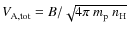 ,
,
 ,
and thus
,
and thus
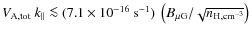 .
Again,
the relevant parameter values can be found in Table 1. In
this low-frequency regime, the damping rate due to ion-neutral
collisions is given by
.
Again,
the relevant parameter values can be found in Table 1. In
this low-frequency regime, the damping rate due to ion-neutral
collisions is given by
(Ferriere et al. 1988).Introducing Eqs. (A.4) and (14) with
 into
Eq. (17) then yields for the cutoff parallel
wavenumber
into
Eq. (17) then yields for the cutoff parallel
wavenumber
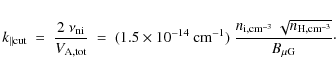
(A.5)
Clearly, this expression is such that ,
which is not quite inside, but not
too far from the validity limit of Eq. (A.4).
,
which is not quite inside, but not
too far from the validity limit of Eq. (A.4).
A comparison with the right-hand side of Eq. (12) immediately shows that
 ,
which
means that the Alfvén wave cascade is cut off by ion-neutral
collisions way before reaching the maximum parallel wavenumber.
Moreover, since positrons can interact resonantly with Alfvén
waves only over a restricted energy range just above
,
which
means that the Alfvén wave cascade is cut off by ion-neutral
collisions way before reaching the maximum parallel wavenumber.
Moreover, since positrons can interact resonantly with Alfvén
waves only over a restricted energy range just above
 ,
corresponding to a restricted wavenumber range just below
,
corresponding to a restricted wavenumber range just below
 (see Sect. 2.1), we may conclude that the Alfvén
wave cascade will produce no waves capable of resonantly interacting
with positrons in the (warm and cold) atomic phases of the ISM.
(see Sect. 2.1), we may conclude that the Alfvén
wave cascade will produce no waves capable of resonantly interacting
with positrons in the (warm and cold) atomic phases of the ISM.
- c.
- Molecular medium
In molecular clouds, Alfvén waves are again damped by ion-neutral collisions. Including the effect of collisions of gas particles on grains, Elmegreen & Fiebig (1993) accurately calculated the minimum scale of Alfvén waves in a molecular cloud of radius R. They found that the maximum value of the product R k is on the order of a few for a typical cloud density .
Since
R typically ranges between 0.01 and 10 pc, this leads to a cutoff
wavenumber
.
Since
R typically ranges between 0.01 and 10 pc, this leads to a cutoff
wavenumber
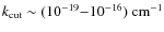 .
Here, too, the smallest scale of the Alfvén wave cascade is
considerably larger than the scales at which resonant interactions
with positrons occur.
.
Here, too, the smallest scale of the Alfvén wave cascade is
considerably larger than the scales at which resonant interactions
with positrons occur.
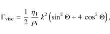
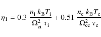
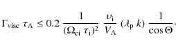

Fast magnetosonic waves
- a.
- Ionized phases
Like Alfvén waves, magnetosonic waves with
are primarily damped by viscous
friction![[*]](/icons/foot_motif.png) . However, because of their compressible
nature, they decay away much faster than Alfvén waves - by a
factor
. However, because of their compressible
nature, they decay away much faster than Alfvén waves - by a
factor
 .
The correct
expression of their viscous damping rate reads
.
The correct
expression of their viscous damping rate reads
where
is the (ion + electron) viscosity coefficient and denotes the viscous damping rate of Alfvén waves
(given by Eq. (A.1))
(Braginskii 1965). The latter is negligible,
except in the limit
denotes the viscous damping rate of Alfvén waves
(given by Eq. (A.1))
(Braginskii 1965). The latter is negligible,
except in the limit
 .
.
With both
and the electron contribution
to  neglected, Eqs. (15) and
(A.6) combine to give
neglected, Eqs. (15) and
(A.6) combine to give
As mentioned below Eq. (A.3), ,
so that
,
so that
 .
It
then follows that, at the injection scale (
.
It
then follows that, at the injection scale (
 ),
),
 .
.
At the transition between the collisional and collisionless ranges (
 ),
),
![\begin{displaymath}\left[ \Gamma_{\rm visc} ~ \tau_{\rm F} \right]_{\lambda_{\rm...
...{L_{\rm inj}}{\lambda_{\rm p}}
\right)^{1/2} \ \sin^2 \Theta ,
\end{displaymath}](/articles/aa/full_html/2009/48/aa09830-08/img351.png)
which can be either smaller or larger than unity, depending on the considered ISM phase and on the propagation angle, .
.
In the hot phase,
![$\left[ \Gamma_{\rm visc} ~ \tau_{\rm F}
\right]_{\lambda_{\rm p}^{-1}} < 1$](/articles/aa/full_html/2009/48/aa09830-08/img352.png) at all propagation angles. This
means that the entire fast magnetosonic cascade manages to reach the
collisionless range beyond
at all propagation angles. This
means that the entire fast magnetosonic cascade manages to reach the
collisionless range beyond
 ,
with only little
or moderate damping.
,
with only little
or moderate damping.
In contrast, in the warm ionized phase,
only for
 ,
with
,
with
 .
If all the waves preserve their propagation angles
across the cascade, then waves with
reach
the collisionless range, whereas those with
.
If all the waves preserve their propagation angles
across the cascade, then waves with
reach
the collisionless range, whereas those with
 are viscous-damped before
reaching
,
and their cutoff wavenumber, given
by Eq. (18), is a decreasing function of :
are viscous-damped before
reaching
,
and their cutoff wavenumber, given
by Eq. (18), is a decreasing function of :
or, numerically,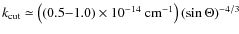 .
However,
the actual situation may not be as clear-cut, as in reality, the
energy transfer down the cascade is accompanied by a randomization of
,
due to both nonlinear interactions between modes with
non-parallel wave vectors and wandering of magnetic field lines.
Yan & Lazarian (2004) estimated that the variation in
is
.
However,
the actual situation may not be as clear-cut, as in reality, the
energy transfer down the cascade is accompanied by a randomization of
,
due to both nonlinear interactions between modes with
non-parallel wave vectors and wandering of magnetic field lines.
Yan & Lazarian (2004) estimated that the variation in
is
 .
At
.
At
 ,
this gives
,
this gives
 ,
which
is small, but not negligible compared to the small values of
,
which
is small, but not negligible compared to the small values of
 .
Ultimately, we cannot rule out the possibility
that even waves with
are cut off by viscous
damping before reaching
.
.
Ultimately, we cannot rule out the possibility
that even waves with
are cut off by viscous
damping before reaching
.
- b.
- Atomic phases
Here, fast magnetosonic waves are damped by ion-neutral collisions, at a rate
with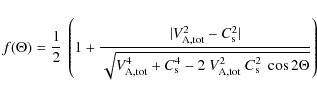
(Ferriere et al. 1988).Substitution of Eqs. (A.10) and (15) into Eq. (18) directly gives for the cutoff wavenumber
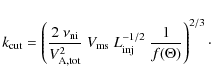
(A.11)
Since in both atomic phases, we may, to
the order of the present approximation, let
in both atomic phases, we may, to
the order of the present approximation, let
 and
and
 in the above equation, whereupon we
obtain
in the above equation, whereupon we
obtain


(A.12)
The fast magnetosonic wave cascade is cut off by ion-neutral collisions way before reaching the small scales at which positrons can be in resonant interaction. - c.
- Molecular medium
Our conclusion is similar to that reached for Alfvén waves.
A.2 Collisionless damping
In Sect. A.1, we saw that, in the ionized phases of the
ISM, the Alfvén wave cascade experiences negligible collisional
damping, which enables it to make it all the way down to the
collisionless range
![]() .
The fast magnetosonic
wave cascade, in contrast, experiences significant collisional
(viscous) damping. In the hot ionized phase, the collisional range
.
The fast magnetosonic
wave cascade, in contrast, experiences significant collisional
(viscous) damping. In the hot ionized phase, the collisional range
![]() is sufficiently narrow that the fast magnetosonic cascade
nevertheless reaches the collisionless range only partially
attenuated. But in the warm ionized phase, where the collisional
range spans roughly eight decades, the fast magnetosonic cascade
completely (or almost completely) decays away before reaching the
collisionless range.
is sufficiently narrow that the fast magnetosonic cascade
nevertheless reaches the collisionless range only partially
attenuated. But in the warm ionized phase, where the collisional
range spans roughly eight decades, the fast magnetosonic cascade
completely (or almost completely) decays away before reaching the
collisionless range.
We now examine collisionless damping in the cases of interest, namely,
for the Alfvén cascade in the hot and warm ionized phases and for
the
fast magnetosonic cascade in the hot ionized phase.![]() In all cases, the dominant collisionless damping mechanism is linear
Landau damping.
In all cases, the dominant collisionless damping mechanism is linear
Landau damping.
Alfvén waves
For Alfvén waves, an approximate expression of the linear Landau
damping rate is (Ginzburg 1961):
![$\displaystyle \times
\left[
\frac{{\upsilon'_{\rm i}}^2}{{\upsilon'_{\rm e}}^2}...
...\
\exp \left( - \frac{V_{\rm A}^2}{2 ~ {\upsilon'_{\rm i}}^2} \right)
\right] ,$](/articles/aa/full_html/2009/48/aa09830-08/img374.png)
where
Multiplying Eq. (A.13) by
Eq. (14) leads to
![$\displaystyle \times
\left[
\frac{{\upsilon'_{\rm i}}^2}{{\upsilon'_{\rm e}}^2}...
...\
\exp \left( - \frac{V_{\rm A}^2}{2 ~ {\upsilon'_{\rm i}}^2} \right)
\right] .$](/articles/aa/full_html/2009/48/aa09830-08/img383.png)
The cutoff of the Alfvén cascade occurs when
In the hot low-B and warm ionized phases, where
![]() ,
the first term inside the square brackets on the
right-hand side of Eq. (A.14) is negligible,
and the relation
,
the first term inside the square brackets on the
right-hand side of Eq. (A.14) is negligible,
and the relation
![]() admits one
solution, given by
admits one
solution, given by
| |
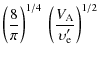
|
||
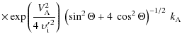
|
(A.15) |
(except in the limit
In the hot high-B phase, where ![]() exceeds
exceeds
![]() by a factor
by a factor
![]() ,
the exponential factor on the
right-hand side of Eq. (A.14) becomes
negligibly small, with the result that
,
the exponential factor on the
right-hand side of Eq. (A.14) becomes
negligibly small, with the result that
![]() at all k (except in the limit
at all k (except in the limit
![]() ,
but in
this limit Alfvén waves are viscous-damped before reaching the
collisionless range;
see Eq. (A.3)). If taken at face value, this
result would lead to the erroneous conclusion that the Alfvén
cascade is not cut off by Landau damping.
,
but in
this limit Alfvén waves are viscous-damped before reaching the
collisionless range;
see Eq. (A.3)). If taken at face value, this
result would lead to the erroneous conclusion that the Alfvén
cascade is not cut off by Landau damping.
The truth is that our expressions for the frequency, transfer time
and damping rate of Alfvén waves are all strictly valid only in the
MHD regime, so that Eq. (A.14) actually breaks
down at
wavenumbers approaching the inverse proton inertial length, ![]() .
The only conclusion that can be drawn from
Eq. (A.14) is that the cutoff of the Alfvén
cascade by Landau damping occurs roughly at the inverse proton
inertial length,
.
The only conclusion that can be drawn from
Eq. (A.14) is that the cutoff of the Alfvén
cascade by Landau damping occurs roughly at the inverse proton
inertial length, ![]() .
.
Fast magnetosonic waves
For fast magnetosonic waves, linear Landau damping proceeds at a rate
(Ginzburg 1961)
![\begin{displaymath}
\Gamma_{\rm LD} =
\sqrt{\frac{\pi}{8}} \ \upsilon'_{\rm i} \...
...2 ~ {\upsilon'_{\rm i}}^2 ~ \cos^2
\Theta}
\right)
\right] ,
\end{displaymath}](/articles/aa/full_html/2009/48/aa09830-08/img393.png)
which, combined with Eq. (15), yields
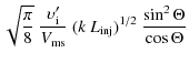
![$\displaystyle \times \left[
\frac{{\upsilon'_{\rm i}}}{{\upsilon'_{\rm e}}}
+ 5...
...c{V_{\rm F}^2}
{2 ~ {\upsilon'_{\rm i}}^2 ~ \cos^2 \Theta}
\right)
\right]\cdot$](/articles/aa/full_html/2009/48/aa09830-08/img396.png)
The cutoff wavenumber, at which

![$\displaystyle \times
\left[
\frac{{\upsilon'_{\rm i}}}{{\upsilon'_{\rm e}}}
+ 5...
...psilon'_{\rm i}}^2 ~ \cos^2
\Theta}
\right)
\right]^{-2} \ L_{\rm inj}^{-1} \ .$](/articles/aa/full_html/2009/48/aa09830-08/img399.png)
Here, the cutoff depends strongly on
The only interstellar phase that needs to be considered here is the
hot ionized phase. In the low-B case,
![]() and the expression within square brackets in
Eq. (A.18) is dominated by the exponential term
(except in the limit
and the expression within square brackets in
Eq. (A.18) is dominated by the exponential term
(except in the limit
![]() ).
Equation (A.18) then reduces to
).
Equation (A.18) then reduces to
![]() .
Despite the strong
.
Despite the strong ![]() -dependence of
-dependence of
![]() ,
we may
conclude that the fast magnetosonic cascade is severely affected by
Landau damping
as soon as it enters the collisionless range and that it globally
decays away shortly below
,
we may
conclude that the fast magnetosonic cascade is severely affected by
Landau damping
as soon as it enters the collisionless range and that it globally
decays away shortly below
![]() .
.
In the high-B case,
![]() ,
the
exponential term drops out from Eq. (A.18), and
the result reads
,
the
exponential term drops out from Eq. (A.18), and
the result reads
![]()
![]() .
Here, Landau damping is less severe, which allows the fast
magnetosonic cascade to globally proceed over roughly three decades
below
.
Here, Landau damping is less severe, which allows the fast
magnetosonic cascade to globally proceed over roughly three decades
below
![]() ,
before vanishing.
,
before vanishing.
Appendix B: Summary of the Monte Carlo algorithm
This section presents a summary of the Monte-Carlo algorithm used
to simulate the collisional transport of positrons in an ISM with
given physical parameters. The method, the equations and the
parameters are described in Sect. 3.
![]() is the
initial positron kinetic energy specified by the user.
is the
initial positron kinetic energy specified by the user.
- 1
- Load the differential and total cross sections, rate of variation of the average scattering-angle and energy-loss rates as functions of positron energy for the given ISM parameters (see Sect. 3.1.1, Eq. (26), Sect. 3.1.2 and references therein).
- 2
- Calculate the distribution function for collisions with
H and annihilation with
 as functions of positron
energy (right hand side of Eq. (29)).
as functions of positron
energy (right hand side of Eq. (29)).
- 3
- Initialize the kinetic parameters of the considered positron
- 3.1
- Set k = 0,
 ,
t0 = 0 and
,
t0 = 0 and
 .
.
- 3.2
- Set the initial direction (isotropic):
- 3.2.1
-
 is chosen randomly between -1 and 1;
- 3.2.2
 is chosen randomly between 0 and
  .
.
- 4
- While the kinetic energy Ek of the positron is larger than 100 eV do
- 4.1
- calculate the gyroradius and the gyrofrequency;
- 4.2
- calculate the scattering time
 (Eq. (31));
- 4.3
- calculate the energy
 at which a collision occurs (Eq. (29));
- 4.4
- calculate the time of flight before the collision
 ;
;
- 4.5
- if
is smaller than
then
- 4.5.1
- calculate the energy lost
 ;
;
- 4.5.2
- calculate the average scattering angle (Eq. (25));
- 4.5.3
- calculate the new pitch angle
 and phase
 (Eqs. (27) and (28));
- 4.5.4
- calculate the new position
 and time
 ;
;
- 4.5.5
- set the energy
 ;
;
- 4.6
- Else if
 is greater than
 then
then
- 4.6.1
- calculate the average scattering angle before the collision (replace
by
in Eq. (25));
- 4.6.2
- calculate the new pitch angle
and phase
before the collision (Eqs. (27) and (28));
- 4.6.3
- calculate the new position
and the time
 ;
;
- 4.6.4
- choose randomly the kind of collision (Eq. (30));
- 4.6.5
- if the interaction is an annihilation then Ek+1 = 0 and go to step 5;
- 4.6.6
- calculate the energy lost in the collision
 (Sect. 3.1.2);
- 4.6.7
- calculate the new pitch angle
and phase
after the collision (Sect. 3.1.2, Eqs. (27) and (28));
- 4.6.8
- set the energy
 ;
;
- 4.7
- End of the kth iteration, set k = k + 1 and go to step 4;
- 5
- Store the final position, time and energy and go to step 3 to process the next positron.
References
- Aharonian, F., Akhperjanian, A. G., Bazer-Bachi, A. R., et al. 2006, ApJ, 636, 777 [NASA ADS] [CrossRef]
- Alexandrova, O., Carbone, V., Veltri, P., & Sorriso-Valvo, L. 2008, ApJ, 674, 1153 [NASA ADS] [CrossRef]
- Armstrong, J. W., Rickett, B. J., & Spangler, S. R. 1995, ApJ, 443, 209 [NASA ADS] [CrossRef]
- Asano, K., Iwamoto, S., & Takahara, F. 2007, ApJS, 168, 268 [NASA ADS] [CrossRef]
- Beacom, J. F., & Yüksel, H. 2006, Phys. Rev. Lett., 97, 071102 [NASA ADS] [CrossRef]
- Bland-Hawthorn, J., & Cohen, M. 2003, ApJ, 582, 246 [NASA ADS] [CrossRef]
- Blumenthal, G. R. & Gould, R. J. 1970, Rev. Mod. Phys., 42, 237 [NASA ADS] [CrossRef]
- Boehm, C., Hooper, D., Silk, J., Casse, M., & Paul, J. 2004, Phys. Rev. Lett., 92, 101301 [NASA ADS] [CrossRef]
- Braginskii, S. I. 1965, Rev. Plasma Phys., 1, 205 [NASA ADS]
- Bussard, R. W., Ramaty, R., & Drachman, R. J. 1979, ApJ, 228, 928 [NASA ADS] [CrossRef]
- Bykov, A. M. 2001, Space Sci. Rev., 99, 317 [NASA ADS] [CrossRef]
- Cardelli, J. A., Meyer, D. M., Jura, M., & Savage, B. D. 1996, ApJ, 467, 334 [NASA ADS] [CrossRef]
- Cesarsky, C. J., & Volk, H. J. 1978, A&A, 70, 367 [NASA ADS]
- Chandran, B. D. G. 2000, Phys. Rev. Lett., 85, 4656 [NASA ADS] [CrossRef]
- Charlton, M., & Humberston, J. W. 2000, Positron Physics (Cambridge, UK: Cambridge University Press)
- Cheng, K. S., Chernyshov, D. O., & Dogiel, V. A. 2006, ApJ, 645, 1138 [NASA ADS] [CrossRef]
- Crutcher, R. M. 1999, ApJ, 520, 706 [NASA ADS] [CrossRef]
- Dermer, C. D. 1984, ApJ, 280, 328 [NASA ADS] [CrossRef]
- Dermer, C. D. 1985, ApJ, 295, 28 [NASA ADS] [CrossRef]
- Diehl, R., Prantzos, N., & von Ballmoos, P. 2006, Nucl. Phys. A, 777, 70 [NASA ADS] [CrossRef]
- Dogel, V. A. & Sharov, G. S. 1985, Soviet Astron. Lett., 11, 346 [NASA ADS]
- Elmegreen, B. G., & Fiebig, D. 1993, A&A, 270, 397 [NASA ADS]
- Everett, J. E., Zweibel, E. G., Benjamin, R. A., et al. 2008, ApJ, 674, 258 [NASA ADS] [CrossRef]
- Farmer, A. J., & Goldreich, P. 2004, ApJ, 604, 671 [NASA ADS] [CrossRef]
- Ferrière, K. 2001, Rev. Mod. Phys., 73, 1031 [NASA ADS] [CrossRef]
- Ferriere, K. M., Zweibel, E. G., & Shull, J. M. 1988, ApJ, 332, 984 [NASA ADS] [CrossRef]
- Ferrière, K., Gillard, W., & Jean, P. 2007, A&A, 467, 611 [NASA ADS] [EDP Sciences] [CrossRef]
- Giacalone, J., & Jokipii, J. R. 1994, ApJ, 430, L137 [NASA ADS] [CrossRef]
- Ginzburg, V., L. 1961, Propagation of Electromagnetic Waves in Plasma (New York: Gordon & Breach)
- Ginzburg, V. L. 1979, Theoretical physics and astrophysics, International Series in Natural Philosophy (Oxford: Pergamon)
- Goldreich, P., & Sridhar, S. 1995, ApJ, 438, 763 [NASA ADS] [CrossRef]
- Gryzinski, M. 1965a, Phys. Rev., 138, 336 [NASA ADS] [CrossRef]
- Gryzinski, M. 1965b, Phys. Rev., 138, 305 [NASA ADS] [CrossRef]
- Gryzinski, M. 1965c, Phys. Rev., 138, 322 [NASA ADS] [CrossRef]
- Guessoum, N., Jean, P., & Gillard, W. 2005, A&A, 436, 171 [NASA ADS] [EDP Sciences] [CrossRef]
- Guessoum, N., Jean, P., & Prantzos, N. 2006, A&A, 457, 753 [NASA ADS] [EDP Sciences] [CrossRef]
- Heiles, C., & Troland, T. H. 2005, ApJ, 624, 773 [NASA ADS] [CrossRef]
- Higdon, J. C., Lingenfelter, R. E., & Rothschild, R. E. 2009, ApJ, 698, 350 [NASA ADS] [CrossRef]
- Huba, J. D. 2006, A collection of plasma physics formulas and data - NRL plasma formulary, Tech. rep., Naval Research Laboratory
- Jean, P., von Ballmoos, P., Knödlseder, J., et al. 2004, in 5th INTEGRAL Workshop on the INTEGRAL Universe, ed. V. Schoenfelder, G. Lichti, & C. Winkler, ESA SP, 552, 51
- Jean, P., Knödlseder, J., Gillard, W., et al. 2006, A&A, 445, 579 [NASA ADS] [EDP Sciences] [CrossRef]
- Keeney, B. A., Danforth, C. W., Stocke, J. T., et al. 2006, ApJ, 646, 951 [NASA ADS] [CrossRef]
- Knödlseder, J., Lonjou, V., Weidenspointner, G., et al. 2005, A&A, 441, 513 [NASA ADS] [EDP Sciences] [CrossRef]
- Kulsrud, R., & Pearce, W. P. 1969, ApJ, 156, 445 [NASA ADS] [CrossRef]
- Lazar, M., Spanier, F., & Schlickeiser, R. 2003, A&A, 410, 415 [NASA ADS] [EDP Sciences] [CrossRef]
- Lazarian, A., & Beresnyak, A. 2006, MNRAS, 373, 1195 [NASA ADS] [CrossRef]
- Lerche, I. 1967, ApJ, 147, 689 [NASA ADS] [CrossRef]
- Lithwick, Y., & Goldreich, P. 2001, ApJ, 562, 279 [NASA ADS] [CrossRef]
- Mac Low, M.-M. & Klessen, R. S. 2004, Rev. Mod. Phys., 76, 125 [NASA ADS] [CrossRef]
- Maurin, D., Taillet, R., & Donato, F. 2002, A&A, 394, 1039 [NASA ADS] [EDP Sciences] [CrossRef]
- McClure-Griffiths, N. M., Ford, A., Pisano, D. J., et al. 2006, ApJ, 638, 196 [NASA ADS] [CrossRef]
- McCray, R., & Kafatos, M. 1987, ApJ, 317, 190 [NASA ADS] [CrossRef]
- Melrose, D. B. 1986, Instabilities in Space and Laboratory Plasmas, Instabilities in Space and Laboratory Plasmas, ed. D. B. Melrose, ISBN 0521305411 (Cambridge, UK: Cambridge University Press, August)
- Morfill, G. E. 1982, MNRAS, 198, 583 [NASA ADS]
- Morris, M., & Serabyn, E. 1996, ARA&A, 34, 645 [NASA ADS] [CrossRef]
- Muno, M. P., Bauer, F. E., Bandyopadhyay, R. M., & Wang, Q. D. 2006, ApJS, 165, 173 [NASA ADS] [CrossRef]
- Ohno, H., & Shibata, S. 1993, MNRAS, 262, 953 [NASA ADS]
- Osterbrock, D. E. 1961, ApJ, 134, 270 [NASA ADS] [CrossRef]
- Parizot, E., Marcowith, A., van der Swaluw, E., Bykov, A. M., & Tatischeff, V. 2004a, A&A, 424, 747 [NASA ADS] [EDP Sciences] [CrossRef]
- Parizot, E., Marcowith, A., van der Swaluw, E., Bykov, A. M., & Tatischeff, V. 2004b, A&A, 424, 747 [NASA ADS] [EDP Sciences] [CrossRef]
- Parizot, E., Cassé, M., Lehoucq, R., & Paul, J. 2005, A&A, 432, 889 [NASA ADS] [EDP Sciences] [CrossRef]
- Prantzos, N. 2006, A&A, 449, 869 [NASA ADS] [EDP Sciences] [CrossRef]
- Ptuskin, V. S., Voelk, H. J., Zirakashvili, V. N., & Breitschwerdt, D. 1997, A&A, 321, 434 [NASA ADS]
- Ragot, B. R. 1999, ApJ, 518, 974 [NASA ADS] [CrossRef]
- Ragot, B. R. 2006, ApJ, 642, 1163 [NASA ADS] [CrossRef]
- Rand, R. J., & Kulkarni, S. R. 1989, ApJ, 343, 760 [NASA ADS] [CrossRef]
- Schlickeiser, R. & Miller, J. A. 1998, ApJ, 492, 352 [NASA ADS] [CrossRef]
- Shull, J. M., & Draine, B. T. 1987, in Interstellar Processes, ed. D. J. Hollenbach, & H. A. Thronson, Jr., Astrophysics and Space Science Library, 134, 283
- Sizun, P., Cassé, M., & Schanne, S. 2006, Phys. Rev. D, 74, 063514 [NASA ADS] [CrossRef]
- Skilling, J. 1975, MNRAS, 173, 255 [NASA ADS]
- Skilling, J., & Strong, A. W. 1976, A&A, 53, 253 [NASA ADS]
- Strong, A. W., Moskalenko, I. V., & Ptuskin, V. S. 2007, Ann. Rev. Nucl. Part. Sci., 57, 285 [NASA ADS] [CrossRef]
- Toptygin, I. N. 1985, Cosmic rays in interplanetary magnetic fields, ed. I. N. Toptygin
- Totani, T. 2006, PASJ, 58, 965 [NASA ADS]
- Veilleux, S., Cecil, G., & Bland-Hawthorn, J. 2005, ARA&A, 43, 769 [NASA ADS] [CrossRef]
- von Ballmoos, P., Guessoum, N., Jean, P., & Knödlseder, J. 2003, A&A, 397, 635 [NASA ADS] [EDP Sciences] [CrossRef]
- Wallyn, P., Durouchoux, P., Chapuis, C., & Leventhal, M. 1994, ApJ, 422, 610 [NASA ADS] [CrossRef]
- Wang, W. 2006, Chin. J. Astron. Astrophys. Suppl., 6, 020000
- Weidenspointner, G., Shrader, C. R., Knödlseder, J., et al. 2006, A&A, 450, 1013 [NASA ADS] [EDP Sciences] [CrossRef]
- Weidenspointner, G., Skinner, G. K., Jean, P., et al. 2008, Nature, 451, L159 [NASA ADS] [CrossRef]
- Wentzel, D. G. 1974, ARA&A, 12, 71 [NASA ADS] [CrossRef]
- Yan, H., & Lazarian, A. 2002, Phys. Rev. Lett., 89, B1102 [NASA ADS] [CrossRef]
- Yan, H., & Lazarian, A. 2004, ApJ, 614, 757 [NASA ADS] [CrossRef]
- Yusef-Zadeh, F., Melia, F., & Wardle, M. 2000, Science, 287, 85 [NASA ADS] [CrossRef]
Footnotes
- ...

- According to Eq. (5),
this condition is automatically satisfied for positrons with
 ,
corresponding to energies
,
corresponding to energies  0.94 GeV.
- ...
scales
- Throughout this paper, the perpendicular and parallel directions are taken with respect to the mean magnetic field direction.
- ... distribution
- The transverse
distribution is
 with
with
 and r the
radius in the xy plane.
and r the
radius in the xy plane.
- ...
friction
- We checked that Joule damping leads to a cutoff
wavenumber several orders of magnitude greater than
.
It only dominates viscous damping at propagation angles
 .
.
- ... phase.
- We will, however, keep in mind the possibility that, in the warm ionized phase, waves with small propagation angles might enter the collisionless regime.
- ... then
- The positron propagates without colliding with a neutral or annihilating with an electron.
- ... then
- A collision with a neutral or an annihilation with an electron occurs.
All Tables
Table 1: Physical parameters of the different ISM phases.
All Figures
|
|
Figure 1:
Energy-loss rates of positrons in a 8000 K plasma with
number densities
|
| Open with DEXTER | |
| In the text | |
|
|
Figure 2:
Kinematic parameters of the scattering in the laboratory frame. The magnetic field |
| Open with DEXTER | |
| In the text | |
|
|
Figure 3:
Spatial distributions of positrons along field lines at the end of their slowing-down period in a warm medium (T = 8000 K and
|
| Open with DEXTER | |
| In the text | |
|
|
Figure 4:
FWHM of the field-aligned distributions of at the end of their
slowing-down period, as functions of their initial kinetic energy. The
hydrogen density is arbitrarily set to
|
| Open with DEXTER | |
| In the text | |
|
|
Figure 5:
Positions of positrons at the end of their slowing-down time in a WIM
taking into account collisional transport in a turbulent magnetic field
(
|
| Open with DEXTER | |
| In the text | |
|
|
Figure 6:
Transverse distributions of positrons at the end of their slowing-down period in a WIM, calculated for maximum turbulent scales
|
| Open with DEXTER | |
| In the text | |
|
|
Figure 7: Minimum and maximum extents of the spatial distributions of positrons reaching 100 eV, along ( top) and perpendicular ( bottom) to the uniform magnetic field, taking into account the turbulent behavior of the field lines as well as realistic values for the density in each ISM phase. |
| Open with DEXTER | |
| In the text | |
|
|
Figure 8: Minimum and maximum extents of the spatial distributions of annihilating positrons, along ( top) and perpendicular ( bottom) to the uniform magnetic field, taking into account the turbulent behavior of the field lines as well as realistic values for the density in each ISM phase. |
| Open with DEXTER | |
| In the text | |
Copyright ESO 2009
Current usage metrics show cumulative count of Article Views (full-text article views including HTML views, PDF and ePub downloads, according to the available data) and Abstracts Views on Vision4Press platform.
Data correspond to usage on the plateform after 2015. The current usage metrics is available 48-96 hours after online publication and is updated daily on week days.
Initial download of the metrics may take a while.