| Issue |
A&A
Volume 508, Number 2, December III 2009
|
|
|---|---|---|
| Page(s) | 933 - 940 | |
| Section | The Sun | |
| DOI | https://doi.org/10.1051/0004-6361/200912946 | |
| Published online | 21 October 2009 | |
A&A 508, 933-940 (2009)
On the physical origin of the second solar spectrum of the Sc II line at 4247 Å
L. Belluzzi
Dipartimento di Astronomia e Scienza dello Spazio, University of Firenze, Largo E. Fermi 2, 50125 Firenze, Italy
Received 21 July 2009 / Accepted 6 August 2009
Abstract
Context. The peculiar three-peak structure of the
linear polarization profile shown in the second solar spectrum by the
Ba II line
at 4554 Å has been interpreted as the result of the different
contributions coming from the barium isotopes with and without
hyperfine structure. In the same spectrum, a triple peak polarization
signal is also observed in the Sc II line
at 4247 Å. Scandium has a single stable isotope (45Sc),
which shows hyperfine structure due to a nuclear spin I=7/2.
Aims. We investigate the possibility of interpreting
the linear
polarization profile shown in the second solar spectrum by this
Sc II line in terms of
hyperfine structure.
Methods. A two-level model atom with hyperfine
structure is
assumed. Adopting an optically thin slab model, the role of atomic
polarization and of hyperfine structure is investigated, avoiding the
complications caused by radiative transfer effects. The slab is assumed
to be illuminated from below by the photospheric continuum, and the
polarization of the radiation scattered at 90![]() is investigated.
is investigated.
Results. The three-peak structure of the scattering
polarization profile observed in this Sc II line
cannot be fully explained in terms of hyperfine structure.
Conclusions. Given the similarities between the
Sc II line at 4247 Å and
the Ba II line at
4554 Å, it is not clear why, within the same modeling
assumptions, only the three-peak Q/I profile
of the barium line can be fully interpreted in terms of hyperfine
structure. The failure to interpret this Sc II
polarization signal raises important questions, whose resolution might
lead to significant improvements in our understanding of the second
solar spectrum. In particular, if the three-peak structure of the
Sc II signal is actually produced
by a physical
mechanism neglected within the approach considered here, it will be
extremely interesting not only to identify this mechanism, but also to
understand why it seems to be less important in the case of the barium
line.
Key words: atomic processes - polarization - scattering - Sun: atmosphere
1 Introduction
The theoretical interpretation of the ``second solar spectrum'', namely the linearly polarized spectrum of the solar radiation coming from quiet regions close to the limb, is presently one of the most intriguing challenges in the field of solar physics. Although the basic physical process at the origin of this spectrum is clear (scattering line polarization), and although several of its properties and peculiarities have been interpreted through the theoretical approaches that have been proposed so far, our understanding of this spectrum remains rather fragmentary, and several features still elude any attempt of interpretation. The main difficulty in the interpretation of the second solar spectrum is that many physical mechanisms are capable of generating or modifying the polarization of the solar radiation, and it is an extremely complicated task to properly quantify their effects in such a complex environment as the solar atmosphere. On the other hand, our knowledge of some of these mechanisms is still rather poor, since they have received attention only recently, both from a theoretical and experimental point of view (e.g., evaluation of the depolarizing collisional rates, development of theoretical frameworks able to account for partial redistribution effects in a self-consistent way, etc.). Nevertheless, the efforts that have been made in this sense are fully justified, because a complete and correct understanding and modeling of the physics underlying the formation of the second solar spectrum will allow us to fully exploit its enormous diagnostic potential, mainly for the investigation of the magnetic fields present in the solar atmosphere (see Trujillo Bueno 2009, for a recent review).Observations performed with instruments having sensitivities on the order of 10-3-10-4 have shown in great detail the spectral richness and complexity of the second solar spectrum (see Stenflo & Keller 1996,1997). Among the profiles observed, those with a three-peak structure have particularly excited the interest and curiosity of the scientific community. Remarkable examples are the three-peak Q/I profiles of the Ca I line at 4227 Å, of the Na I D2 line at 5889 Å, and of the Ba II D2 line at 4554 Å. The intensity spectrum and the second solar spectrum of the Na I and Ba II D2 lines are shown in the first two panels of Fig. 1.
![\begin{figure}
\par\includegraphics[width=18cm]{12946fg1.eps}
\end{figure}](/articles/aa/full_html/2009/47/aa12946-09/img18.png)
|
Figure 1: Three spectral lines showing a three-peak Q/I profile in the second solar spectrum: the Na I D2 line at 5889 Å ( left), the Ba II line at 4554 Å ( middle), and the Sc II line at 4247 Å ( right). The dashed line in the lower panels represents the polarization level of the continuum. All the observations are taken from Gandorfer (2000,2002). |
| Open with DEXTER | |
The three-peak structure shown by the Ba II D2 line
has been explained in terms of the presence of barium isotopes both
with and without hyperfine structure (HFS) (see Belluzzi et al. 2007; Stenflo 1997).
In particular, it has been shown that the two secondary peaks in the
wings of the Q/I profile
are due to the isotopes with HFS (![]() 18% in abundance), while the
central,
higher peak is produced by the isotopes without HFS (
18% in abundance), while the
central,
higher peak is produced by the isotopes without HFS (![]() 82% in
abundance). Taking into account the effect of the HFS shown by this
rather small fraction of barium isotopes, the observed three-peak
profile could be reproduced to very high accuracy, even within the
simplifying modeling assumption of the so-called optically thin slab
model (i.e., neglecting radiative transfer effects).
82% in
abundance). Taking into account the effect of the HFS shown by this
rather small fraction of barium isotopes, the observed three-peak
profile could be reproduced to very high accuracy, even within the
simplifying modeling assumption of the so-called optically thin slab
model (i.e., neglecting radiative transfer effects).
As can be observed in the right panel of Fig. 1, also the Sc II line at 4247 Å shows in the second solar spectrum a three-peak Q/I profile. In contrast to the Q/I profile produced by the Ba II D2 line, which shows a central peak (due to the isotopes without HFS) of amplitude much larger than that of the lateral peaks, the three peaks exhibited by this scandium signal have approximately the same amplitude. This peculiarity strongly suggests that the three-peak structure of this signal might also be due to HFS, since scandium has a single stable isotope, which shows HFS (see Sect. 2.2). This possibility is strengthened by the wavelength separation between the lateral peaks being very similar to that observed in the Q/I profile of the Ba II D2 line, and by this scandium line in the intensity spectrum being very similar to the Ba II D2 line. We note that these latter circumstances do not hold in the case of the Na I D2 line: the sodium line is much stronger and broader in the intensity spectrum, and the wavelength separation between the lateral peaks shown by the Q/I profile is much larger than for either barium or scandium. Indeed, it has already been observed that the three-peak structure of the Na I D2 line cannot be explained only in terms of the HFS exhibited by the single stable isotope of sodium, but that its interpretation seems to require the inclusion of other physical ``ingredients'' such as ``super-interferences'' and lower level polarization (see Landi Degl'Innocenti 1998), and/or the effects of partial redistribution in frequency (see Holzreuter et al. 2005), and/or the enhancement of the line-center scattering polarization peak by vertical magnetic fields (see Trujillo Bueno et al. 2002). For the reasons explained above, we considered it worthwhile to investigate whether the peculiar three-peak structure of this scandium Q/I signal might be explained in terms of HFS, within a modeling approach similar to that proposed by Belluzzi et al. (2007) for the Ba II D2 line.
2 Formulation of the problem
2.1 The two-level atom with hyperfine structure
It is well-known that hyperfine structure is produced by the influence
of the nucleus on the energy levels of the atom. On the one hand, this
influence is related to the nuclei of the various isotopes having
slightly different volumes and masses (isotopic effect), and on the
other hand, to the coupling of the nuclear spin ![]() with the total angular momentum
with the total angular momentum ![]() of the electronic cloud (nuclear spin effect).
We note that it is customary to speak about hyperfine structure tout
court when referring to the nuclear spin effect only.
of the electronic cloud (nuclear spin effect).
We note that it is customary to speak about hyperfine structure tout
court when referring to the nuclear spin effect only.
In the absence of magnetic fields, using Dirac's notation, the
energy eigenvectors of an atomic system with HFS can be written in the
form ![]() ,
where
,
where ![]() represents a set of inner quantum numbers (specifying the electronic
configuration and, if the atomic system is described by the L-S
coupling scheme, the total electronic orbital, and spin angular
momenta), F is the quantum number associated with
the total angular momentum operator (electronic plus nuclear:
represents a set of inner quantum numbers (specifying the electronic
configuration and, if the atomic system is described by the L-S
coupling scheme, the total electronic orbital, and spin angular
momenta), F is the quantum number associated with
the total angular momentum operator (electronic plus nuclear: ![]() ),
and f is the quantum number associated with
the projection of
),
and f is the quantum number associated with
the projection of ![]() along the quantization axis.
It is possible to demonstrate that the HFS Hamiltonian, describing the
interaction between the nuclear spin and the electronic angular
momentum,
can be expressed as a series of electric and magnetic multipoles
(see, for example, Kopfermann 1958).
In this investigation, we retain only the first two terms
(magnetic-dipole
and electric-quadrupole), which are given by
along the quantization axis.
It is possible to demonstrate that the HFS Hamiltonian, describing the
interaction between the nuclear spin and the electronic angular
momentum,
can be expressed as a series of electric and magnetic multipoles
(see, for example, Kopfermann 1958).
In this investigation, we retain only the first two terms
(magnetic-dipole
and electric-quadrupole), which are given by
where ![]() and
and ![]() are the
magnetic-dipole and the electric-quadrupole HFS constants,
respectively, and where
are the
magnetic-dipole and the electric-quadrupole HFS constants,
respectively, and where
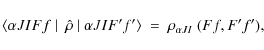
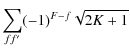
| K=F(F+1)-J(J+1)-I(I+1) . | (2) |
We describe the atomic system by means of the density matrix formalism, a robust theoretical framework very suitable for handling atomic polarization phenomena (population imbalances and quantum interferences between pairs of magnetic sublevels) that can be induced in the atomic system (for example by an anisotropic incident radiation field). Since the upper and lower levels of the Sc II line at 4247 Å pertain to singlet terms (this is the only line of the multiplet), we consider a simple two-level model atom with HFS. Following Landi Degl'Innocenti & Landolfi (2004, hereafter LL04), we describe the atom through the density matrix elements
where
|
|
= | 
|
|
|
(4) |
The statistical equilibrium equations (SEE), and the radiative transfer coefficients for a two-level atom with HFS, in the spherical statistical tensor representation can be found in LL04. Here we write only the expression of the emission coefficient (in the absence of magnetic fields)
with ![]() (corresponding respectively to the Stokes parameters
I,Q,U, and V),
(corresponding respectively to the Stokes parameters
I,Q,U, and V),
![]() the number density of atoms,
the number density of atoms,
![]() the Einstein coefficient
for spontaneous emission,
the Einstein coefficient
for spontaneous emission, ![]() a
geometrical tensor (see Sect. 5.11 of LL04), and
a
geometrical tensor (see Sect. 5.11 of LL04), and ![]() the (complex) profile of the line.
The indices
the (complex) profile of the line.
The indices ![]() and u have the usual meaning of lower and upper
(level), respectively.
and u have the usual meaning of lower and upper
(level), respectively.
It is important to recall that Eq. (5), and the SEE
needed to find the spherical statistical tensors ![]() are
valid under the flat-spectrum approximation.
For a two-level atom with HFS, this approximation requires that the
incident radiation field should be flat (i.e., independent of
frequency) across a spectral interval
are
valid under the flat-spectrum approximation.
For a two-level atom with HFS, this approximation requires that the
incident radiation field should be flat (i.e., independent of
frequency) across a spectral interval ![]() larger than the frequency intervals among the HFS levels, and larger
than the inverse lifetimes of the same levels. Given the small
frequency separation between the various HFS levels (see Fig. 2), this
appears to be a good approximation for the Sc II line
under investigation.
larger than the frequency intervals among the HFS levels, and larger
than the inverse lifetimes of the same levels. Given the small
frequency separation between the various HFS levels (see Fig. 2), this
appears to be a good approximation for the Sc II line
under investigation.
2.2 The atomic model
Scandium has only one stable isotope (45Sc), of nuclear spin I=7/2. The Sc II line at 4247 Å originates from the transition between the levels 3d4s 1D2 (lower level) and 3d4p 1D2 (upper level). The Einstein coefficient for spontaneous emission isTable 1: Magnetic dipole and electric quadrupole HFS constants of the levels considered in this investigation.
The laboratory positions and the relative strengths of the various HFS components are shown in the lower panel of Fig. 2.![\begin{figure}
\par\includegraphics[width=8.8cm]{12946fg2.eps}\vspace{2mm}
\end{figure}](/articles/aa/full_html/2009/47/aa12946-09/img52.png)
|
Figure 2: Upper panel: Grotrian diagram showing the terms, the fine structure, and the hyperfine structure levels considered in the atomic model (the separation between the two J-levels is not on scale). The 13 HFS components of the line under investigation are drawn in the diagram. Lower panel: laboratory positions and relative strengths of the various HFS components, broadened by their natural width. Note that only twelve components are visible since two are blended. The zero of the wavelength scale is at 4246.82 Å. |
| Open with DEXTER | |
Despite the simplicity of the atomic model considered (two-level atom),
because of the high values of the quantum numbers involved, the SEE
form a set of 3200 equations in 3200 unknowns (the
various spherical statistical tensors ![]() of the upper and lower levels). To reduce the amount of numerical
calculations involved in the solution of this set of equations, we
limit ourselves to considering only the spherical statistical tensors
with
of the upper and lower levels). To reduce the amount of numerical
calculations involved in the solution of this set of equations, we
limit ourselves to considering only the spherical statistical tensors
with ![]() ,
thus reducing the SEE to a set of 278 equations. Because of
the low value of the anisotropy factor that we assume for the radiation
field (see following subsection), the statistical tensors of higher
rank are found to be almost two orders of magnitude smaller, so that
the results obtained within this approximation do not show any
appreciable difference with respect to those obtained by carrying out
the complete calculations.
,
thus reducing the SEE to a set of 278 equations. Because of
the low value of the anisotropy factor that we assume for the radiation
field (see following subsection), the statistical tensors of higher
rank are found to be almost two orders of magnitude smaller, so that
the results obtained within this approximation do not show any
appreciable difference with respect to those obtained by carrying out
the complete calculations.
2.3 The optically thin slab model
![\begin{figure}
\par\includegraphics[width=8cm]{12946fg3.eps}\end{figure}](/articles/aa/full_html/2009/47/aa12946-09/img55.png)
|
Figure 3: Geometry of the problem being investigated. |
| Open with DEXTER | |
where ![]() is the cosine of the heliocentric angle.
The former quantity is the mean intensity of the radiation field
(averaged over all directions), the second quantifies the anisotropy of
the radiation field (imbalance between vertical and horizontal
illumination). The mean intensity of the radiation field can also be
expressed in terms of the average number of photons per mode,
is the cosine of the heliocentric angle.
The former quantity is the mean intensity of the radiation field
(averaged over all directions), the second quantifies the anisotropy of
the radiation field (imbalance between vertical and horizontal
illumination). The mean intensity of the radiation field can also be
expressed in terms of the average number of photons per mode, ![]() ,
while the anisotropy degree is often quantified through the so-called
anisotropy factor, w. These new, non-dimensional
quantities are related to J00
and J20
by the equations
,
while the anisotropy degree is often quantified through the so-called
anisotropy factor, w. These new, non-dimensional
quantities are related to J00
and J20
by the equations
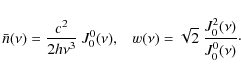
|
(7) |
We calculate the values of
Taking into account the atomic weight of scandium, assuming a
temperature
of 6000 K, and neglecting microturbulent velocity, we obtain
for this line a Doppler width, ![]() ,
given by
,
given by
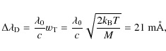
|
(8) |
where
| Figure 4:
Fractional atomic alignment |
|
| Open with DEXTER | |
2.4 Polarization of the emergent spectral line radiation
Once the SEE have been written down and solved numerically, we can calculate the radiative transfer coefficients according to the equations of Sect. 7.9 of LL04. We consider the radiation scattered by the slab at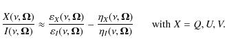
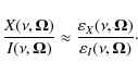
The first and second terms in the right-hand side of Eq. (9) represent the contribution to the emergent radiation due to processes of selective emission and selective absorption (dichroism) of polarization components, respectively.
We note that while the lower level of Ba II
D2, with J=1/2, can carry
alignment only because of the presence of HFS, the lower level of this
scandium line, with J=2, can be polarized also
neglecting HFS. As a consequence, while in the case of the Ba
II D2 line
the lower level results to be significantly less polarized than the
upper level (see Belluzzi
et al. 2007), in this scandium line the upper and
lower levels carry the same amount of atomic polarization![]() (see Fig. 4).
Although the contribution of dichroism is thus expected to be more
important in this line than in the Ba II
D2 line, we start our investigation by
neglecting it.
(see Fig. 4).
Although the contribution of dichroism is thus expected to be more
important in this line than in the Ba II
D2 line, we start our investigation by
neglecting it.
![\begin{figure}
\par\includegraphics[width=18cm]{12946fg5.eps}
\end{figure}](/articles/aa/full_html/2009/47/aa12946-09/img73.png)
|
Figure 5:
Left panel: fractional polarization profile
for the Ba II line at
4554 Å, obtained by applying Eq. (10) (without
continuum).
The values of |
| Open with DEXTER | |
Some results obtained taking into account dichroism effects (i.e., applying Eq. (9)) will be shown in Sect. 3.4.
We recall that the emission coefficient given in Eq. (5) includes only
line processes. To reproduce, albeit qualitatively, the observed
profile, we need to add the contribution of the continuum. Assuming
that the continuum is constant across the line, we have
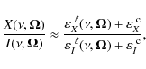
where the superscripts ``c'' and ``
We point out that the three-peak structure of the Q/I profile shown by the Ba II D2 line could be reproduced by Belluzzi et al. (2007) within the constraints of the same modeling assumptions and approximations outlined above. However, we note that this ionized scandium line is a rather strong spectral line: as for Ba II D2, the wings of this line originate in the photosphere, while the line core originates in the high photosphere/low chromosphere. The optically thin slab model considered in this paper is therefore just a first order approximation. Nevertheless, as previously stated, it allows us to take into account in a very rigorous way the relevant atomic aspects of the problem, avoiding the complications produced by radiative transfer effects.
![\begin{figure}
\par\includegraphics[width=17.5cm,clip]{12946fg6.eps}
\end{figure}](/articles/aa/full_html/2009/47/aa12946-09/img78.png)
|
Figure 6:
Left panel: theoretical profiles obtained
including the continuum contribution to the intensity. The various
profiles have been obtained by assuming |
| Open with DEXTER | |
3 Results
3.1 Three-peak structure of the Ba II D2 line Q/I profile
As discussed in Belluzzi et al.
(2007), the presence of barium isotopes both with and without
HFS is understood to be important in explaining the three-peak
structure of the Q/I profile
shown in the second solar spectrum by the Ba II
D2 line. In particular, the central
peak is due to the isotopes without HFS, while the two lateral peaks
seem to be caused by the depolarizing effect of the isotopes with HFS (135Ba
and 137Ba), combined with the effect of the
continuum, which depolarizes the wings of the line.
The fractional polarization profile plotted in the left panel of
Fig. 5
clearly shows the depolarizing effect of the isotopes with HFS, as well
as the polarization enhancement at line center due to the isotopes
without HFS.
This profile was obtained by applying Eq. (10) (i.e.,
neglecting the continuum) to the case of the Ba II
D2 line, assuming for ![]() ,
w, and
,
w, and ![]() the values corresponding to a slab of barium ions at 6000 K,
located 1000 km above the solar surface. Starting from this
fractional polarization profile, and adding the contribution of the
continuum, Belluzzi et al.
(2007) were able to obtain a good fit to the observed
three-peak Q/I profile.
the values corresponding to a slab of barium ions at 6000 K,
located 1000 km above the solar surface. Starting from this
fractional polarization profile, and adding the contribution of the
continuum, Belluzzi et al.
(2007) were able to obtain a good fit to the observed
three-peak Q/I profile.
The fundamental role of the isotopes without HFS in producing the higher central peak of the observed linear polarization profile can be clearly appreciated from the middle panel of Fig. 5. Here the same fractional polarization profile as in the left panel of Fig. 5 (without continuum) is plotted assuming that only the isotope 137Ba (with HFS) is present (100% in abundance). Comparing the two profiles, it is noticeable that although a polarization enhancement can be observed at line center also when only 137Ba is present, this is much larger when the isotopes without HFS are also taken into account. In particular, if these isotopes are considered, the polarization at line center reaches the same value as in the far wings. This is an important peculiarity, since in this case there is no way, by adding the continuum, to obtain three peaks of the same amplitude (such as those observed in the Sc II line). On the other hand, this would be possible if, hypothetically, only the isotope 137Ba were present.
3.2 Three-peak structure of the Sc II 4247 Å line Q/I profile
As previously pointed out, scandium has a single stable isotope, with
HFS, which is consistent with the interpretation of this scandium
signal, showing three peaks of the same amplitude, in terms of HFS.
Applying Eq. (10),
and using the values previously calculated for ![]() ,
w, and
,
w, and ![]() ,
we find the fractional polarization profile shown in the right panel of
Fig. 5.
The profile clearly shows the depolarizing effect of HFS
,
we find the fractional polarization profile shown in the right panel of
Fig. 5.
The profile clearly shows the depolarizing effect of HFS![]() , but the polarization
enhancement at line-center, which produces the central peak, is by far
less evident than in the case of 137Ba.
On the one hand, this is because the HFS components of 137Ba
are gathered into two well separated groups (because of the large HFS
splitting of the ground level), while the HFS components of scandium
are gathered into a single group at line center, spreading out over a
narrow wavelength interval of about 15 mÅ (see the middle and
right panels of Fig. 5,
and Fig. 2).
On the other hand, the smaller Doppler width assumed for barium (much
heavier than scandium) contributes to making the line-core enhancement
of the corresponding fractional polarization profile far more evident.
, but the polarization
enhancement at line-center, which produces the central peak, is by far
less evident than in the case of 137Ba.
On the one hand, this is because the HFS components of 137Ba
are gathered into two well separated groups (because of the large HFS
splitting of the ground level), while the HFS components of scandium
are gathered into a single group at line center, spreading out over a
narrow wavelength interval of about 15 mÅ (see the middle and
right panels of Fig. 5,
and Fig. 2).
On the other hand, the smaller Doppler width assumed for barium (much
heavier than scandium) contributes to making the line-core enhancement
of the corresponding fractional polarization profile far more evident.
As in the case of barium, to reproduce the observed profile,
it is necessary to include the effect of the continuum. By so doing,
the value of the fractional polarization decreases in the wings of the
line, and a two-peak profile with a small hump at line center is
obtained. The left panel of Fig. 6 shows the
profiles that result when assuming different values of ![]() ,
where
,
where ![]() is the maximum value of
is the maximum value of ![]() in the wavelength range considered. A value of
in the wavelength range considered. A value of ![]() on the order of 10-3 is needed to obtain similar
polarization values in the wing peaks and the line-core. Because of the
small enhancement exhibited by the fractional polarization profile at
line center, by setting
on the order of 10-3 is needed to obtain similar
polarization values in the wing peaks and the line-core. Because of the
small enhancement exhibited by the fractional polarization profile at
line center, by setting ![]() we actually obtain a profile with three peaks of the same amplitude
(see the middle panel of Fig. 6).
we actually obtain a profile with three peaks of the same amplitude
(see the middle panel of Fig. 6).
To reproduce the amplitude of the central peak (![]() 0.46%,
according to the observation of Gandorfer 2002), and the polarization
level of the continuum at the wavelength of this line (
0.46%,
according to the observation of Gandorfer 2002), and the polarization
level of the continuum at the wavelength of this line (![]() 0.23%), we
have to set w=0.11 and
0.23%), we
have to set w=0.11 and ![]() .
Assuming that
.
Assuming that ![]() (which is a rather realistic value for a spectral line such as that
under investigation), we obtain the theoretical profile plotted in the
right panel of Fig. 6.
This profile indeed shows a three-peak structure, but its width can be
immediately noticed to be much smaller than that of the observed
profile. In particular, in the observed profile the wavelength
separations between the two dips and between the two lateral peaks are
about 90 mÅ and 190 mÅ, respectively, while in the
theoretical profile
they are about 75 mÅ and 110 mÅ, respectively.
Moreover, while the amplitude of the dip at longer wavelengths (the
``red'' dip) is very similar to the observed one, the amplitude of the
``blue''
dip is much smaller.
(which is a rather realistic value for a spectral line such as that
under investigation), we obtain the theoretical profile plotted in the
right panel of Fig. 6.
This profile indeed shows a three-peak structure, but its width can be
immediately noticed to be much smaller than that of the observed
profile. In particular, in the observed profile the wavelength
separations between the two dips and between the two lateral peaks are
about 90 mÅ and 190 mÅ, respectively, while in the
theoretical profile
they are about 75 mÅ and 110 mÅ, respectively.
Moreover, while the amplitude of the dip at longer wavelengths (the
``red'' dip) is very similar to the observed one, the amplitude of the
``blue''
dip is much smaller.
The only way to increase the width of the theoretical profile
is to assume a larger value of the Doppler width. In the case of
barium, to reproduce the observed profile it was necessary to assume a
Doppler width of 30 mÅ, corresponding to a temperature of
6000 K and a microturbulent velocity of
1.8 km s-1 (see Belluzzi et al. 2007).
In the left panel of Fig. 7, the barium
fractional polarization profiles, obtained by assuming ![]() mÅ
(dotted line) and
mÅ
(dotted line) and ![]() mÅ
(solid line) are shown: increasing the Doppler width, the wavelength
separation between the two dips is increased, but the two-dip structure
of the profile is not lost. In the middle panel of Fig. 7, we plot the
fractional polarization profiles of the scandium line, obtained by
assuming
mÅ
(solid line) are shown: increasing the Doppler width, the wavelength
separation between the two dips is increased, but the two-dip structure
of the profile is not lost. In the middle panel of Fig. 7, we plot the
fractional polarization profiles of the scandium line, obtained by
assuming ![]() mÅ
(dotted line) and
mÅ
(dotted line) and ![]() mÅ
(solid line), the latter corresponding to a temperature of
6000 K and a microturbulent velocity of
1.8 km s-1. Increasing the
Doppler width, the fractional polarization profile shows a
significantly larger depolarizing feature, but the small polarization
enhancement at line core, and therefore the three-peak structure of the
polarization profile obtained by adding the continuum, are almost
completely lost (see the middle and right panels of Fig. 7).
mÅ
(solid line), the latter corresponding to a temperature of
6000 K and a microturbulent velocity of
1.8 km s-1. Increasing the
Doppler width, the fractional polarization profile shows a
significantly larger depolarizing feature, but the small polarization
enhancement at line core, and therefore the three-peak structure of the
polarization profile obtained by adding the continuum, are almost
completely lost (see the middle and right panels of Fig. 7).
![\begin{figure}
\par\includegraphics[width=18cm]{12946fg7.eps}
\end{figure}](/articles/aa/full_html/2009/47/aa12946-09/img82.png)
|
Figure 7:
Left panel: fractional polarization profiles
for the Ba II line at
4554 Å, obtained by applying Eq. (10) (without
continuum), assuming |
| Open with DEXTER | |
![\begin{figure}
\par\includegraphics[width=18cm]{12946fg8.eps}
\end{figure}](/articles/aa/full_html/2009/47/aa12946-09/img83.png)
|
Figure 8:
Left panel: theoretical polarization profiles
obtained in the presence of a unimodal microturbulent magnetic field of
various intensities. All the profiles are calculated by using
Eq. (11),
assuming for the free parameters the same values as in the right panel
of Fig. 6.
The solid-line profile is the same as in the right panel of
Fig. 6.
Middle panel: |
| Open with DEXTER | |
3.3 The effect of a unimodal microturbulent magnetic field
The left panel of Fig. 8 shows the theoretical linear polarization profiles obtained according to Eq. (11), in the presence of a unimodal microturbulent magnetic field of various intensities. A useful estimate of the spectral line sensitivity to the Hanle effect can be obtained by calculating the critical fields of the upper and lower levels (see, for example, Trujillo Bueno 2001)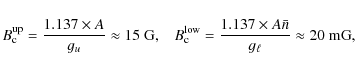
|
(12) |
where the Einstein coefficient for spontaneous emission must be expressed in units of 107 s-1. In agreement with the previous estimate, we observe an increase of the polarization, due to the lower-level Hanle effect, for magnetic fields between 10 mG and 1 G. The polarization is found to increase by a larger amount at the wavelength positions of both the central peak and the blue dip, than of the red dip. If the continuum is changed, so that the wing peaks have the same amplitude as the central peak, a three-peak structure might possibly be recovered, but a red dip much deeper than the blue one would be found, in disagreement with the observation. We point out that the lower-level Hanle effect is particularly evident in this scandium line because, as previously observed, the lower level carries the same amount of atomic polarization as the upper level (in the Ba II D2 line, where the lower level is much less polarized than the upper level, this effect cannot be observed).
If the magnetic field is further increased, the upper level
Hanle effect becomes dominant, and a depolarization at the line core is
observed.
We note that for magnetic fields on the order of 100 G, the
polarization at line center becomes lower than in the far wings (i.e.,
lower than the continuum), although always remaining positive. A
saturation regime is reached for fields of about 200 G.
Even though for fields on the order of 50 G, a three-peak
structure can still be recovered by adjusting the parameters (w
and ![]() ),
nevertheless the observed profile cannot be reproduced.
In particular, the width of the theoretical profile does not increase
appreciably with the magnetic field intensity, so that the disagreement
with the observation previously discussed cannot be solved.
),
nevertheless the observed profile cannot be reproduced.
In particular, the width of the theoretical profile does not increase
appreciably with the magnetic field intensity, so that the disagreement
with the observation previously discussed cannot be solved.
In conclusion, within our modeling assumptions, which also include the effect of a unimodal microturbulent magnetic field, it is not possible to reproduce the observed Q/I profile.
3.4 Results obtained including dichroism
In the middle panel of Fig. 8, the ![]() profile
is plotted. In the line-core, it exhibits an anti-symmetrical shape,
while in the far wings, because of the presence of lower level
polarization, it reaches an asymptotic value that differs from zero.
The profile obtained by applying Eq. (9) is plotted
with a solid line in the right panel of Fig. 8.
Comparing this profile with the one previously obtained by means of
Eq. (10)
(plotted with a dotted line in the same figure), an overall shift
towards higher values of polarization is discernible, in addition to a
slightly different substructure in the line-core, that, however, does
not provide a more accurate fit to the observed profile. The inclusion
of dichroism does not modify the width of the profile.
By also including dichroism, if we increase the width of the profile by
assuming a larger value of the Doppler width, the three-peak structure
of the profile is found to be lost.
profile
is plotted. In the line-core, it exhibits an anti-symmetrical shape,
while in the far wings, because of the presence of lower level
polarization, it reaches an asymptotic value that differs from zero.
The profile obtained by applying Eq. (9) is plotted
with a solid line in the right panel of Fig. 8.
Comparing this profile with the one previously obtained by means of
Eq. (10)
(plotted with a dotted line in the same figure), an overall shift
towards higher values of polarization is discernible, in addition to a
slightly different substructure in the line-core, that, however, does
not provide a more accurate fit to the observed profile. The inclusion
of dichroism does not modify the width of the profile.
By also including dichroism, if we increase the width of the profile by
assuming a larger value of the Doppler width, the three-peak structure
of the profile is found to be lost.
4 Conclusions
In terms of the same modeling approximations adopted by Belluzzi et al. (2007) to reproduce the three-peak Q/I profile observed in the second solar spectrum of the Ba II D2 line, it is impossible to reproduce the similar three-peak linear polarization profile exhibited in the same spectrum by the Sc II line at 4247 Å. This is a surprising result given the similarities between the two lines in the intensity spectrum, and that the only stable isotope of scandium shows hyperfine structure, which is the physical aspect responsible for the triple peak structure of the Ba II D2 line Q/I profile. The possibility of reproducing the polarization signal of this ionized scandium line in terms of hyperfine structure was also suggested by the three peaks having the same amplitude, a circumstance that appears to be in perfect agreement with the absence of scandium isotopes without hyperfine structure. We are indeed able to obtain a Q/I profile with three peaks of the same amplitude, but unfortunately its width is found to be considerably smaller than that of the observed profile. Moreover, while the red dip can be reproduced quite well, the depth of the blue one is much smaller than in the observation. The only way to increase the width of the profile is to assume alarger Doppler width, but, in this case, the three peak structure is rapidly lost. We investigated the effect of a microturbulent magnetic field, as well as the effect of dichroism, but they both do not seem to be able to explain the disagreement between our theoretical result and the observation. Nevertheless, it is important to point out that the lower level of this line, being polarizable irrespective of the hyperfine structure (
The author wishes to express his gratitude to Egidio Landi Degl'Innocenti and Javier Trujillo Bueno for several scientific discussions, and for helpful comments and suggestions.
References
- Belluzzi, L., Trujillo Bueno, J., & Landi Degl'Innocenti, E. 2007, ApJ, 666, 588 [NASA ADS] [CrossRef]
- Gandorfer, A. 2000, The Second Solar Spectrum: A High Resolution Polarimetric Survey of Scattering Polarization at the Solar Limb in Graphical Representation, Vol. I: 4625 Å to 6995 Å (Zürich: vdf ETH)
- Gandorfer, A. 2002, The Second Solar Spectrum: A High Resolution Polarimetric Survey of Scattering Polarization at the Solar Limb in Graphical Representation, Vol. II: 3910 Å to 4630 Å (Zürich: vdf ETH)
- Holzreuter, R., Fluri, D. M., & Stenflo, J. O. 2005, A&A, 434, 713 [NASA ADS] [EDP Sciences] [CrossRef]
- Kopfermann, H. 1958, Nuclear Moments (New York: Academic Press)
- Landi Degl'Innocenti, E. 1998, Nature, 392, 256 [NASA ADS] [CrossRef]
- Landi Degl'Innocenti, E., & Landolfi, M. 2004, Polarization in Spectral Lines (Dordrecht: Kluwer) (LL04)
- Pierce, K. 2000, in Allen's Astrophysical Quantities, ed. A. N. Cox 4th edn. (New York: Springer), 355
- Ralchenko, Yu., Kramida, A. E., Reader, J., & NIST ASD Team 2008, NIST Atomic Spectra Database (version 3.1.4) (Gaithersburg, MD.: NIST) [Online]
- Stenflo, J. O. 1997, A&A, 324, 344 [NASA ADS]
- Stenflo, J. O., & Keller, C. U. 1996, Nature, 382, 588 [NASA ADS] [CrossRef]
- Stenflo, J. O., & Keller, C. U. 1997, A&A, 321, 927 [NASA ADS]
- Trujillo Bueno, J. 2001, Atomic Polarization and the Hanle effect in Advanced Solar Polarimetry: Theory, Observations and Instrumentation, ed. M. Sigwarth, ASP Conf. Ser., 236, 161
- Trujillo Bueno, J. 2003, New Diagnostic Windows on the Weak Magnetism of the Solar Atmosphere in Solar Polarization, Proceeding of the Conference held 30 September - 4 October 2002 at Tenerife, Canary Islands, Spain, ed. J. Trujillo Bueno, & J. Sanchez Almeida, ASP Conf. Ser., 307, 407
- Trujillo Bueno, J. 2009, The Magnetic Sensitivity of the Second Solar Spectrum, in Solar Polarization 5, ed. S. Berdyugina, K. N. Nagendra, & R. Ramelli, ASP Conf. Ser., 405, 65
- Trujillo Bueno, J., Casini, R., Landolfi, M., & Landi Degl'Innocenti, E. 2002, ApJ, 566, L53 [NASA ADS] [CrossRef]
- Villemoes, P., van Leeuwen, R., Arnesen, A., et al. 1992, Phys. Rev. A, 45, 6241 [NASA ADS] [CrossRef]
Footnotes
- ... polarization
![[*]](/icons/foot_motif.png)
- Collisions will be neglected throughout this investigation.
- ... HFS
- Note that if HFS had been neglected, the fractional polarization profile calculated considering only the line processes (no continuum) would have been constant with wavelength, as it is clear from Belluzzi et al. (2007), where the results obtained considering only 138Ba (without HFS) are shown.
All Tables
Table 1: Magnetic dipole and electric quadrupole HFS constants of the levels considered in this investigation.
All Figures
|
|
Figure 1: Three spectral lines showing a three-peak Q/I profile in the second solar spectrum: the Na I D2 line at 5889 Å ( left), the Ba II line at 4554 Å ( middle), and the Sc II line at 4247 Å ( right). The dashed line in the lower panels represents the polarization level of the continuum. All the observations are taken from Gandorfer (2000,2002). |
| Open with DEXTER | |
| In the text | |
|
|
Figure 2: Upper panel: Grotrian diagram showing the terms, the fine structure, and the hyperfine structure levels considered in the atomic model (the separation between the two J-levels is not on scale). The 13 HFS components of the line under investigation are drawn in the diagram. Lower panel: laboratory positions and relative strengths of the various HFS components, broadened by their natural width. Note that only twelve components are visible since two are blended. The zero of the wavelength scale is at 4246.82 Å. |
| Open with DEXTER | |
| In the text | |
|
|
Figure 3: Geometry of the problem being investigated. |
| Open with DEXTER | |
| In the text | |
| |
Figure 4:
Fractional atomic alignment |
| Open with DEXTER | |
| In the text | |
|
|
Figure 5:
Left panel: fractional polarization profile
for the Ba II line at
4554 Å, obtained by applying Eq. (10) (without
continuum).
The values of |
| Open with DEXTER | |
| In the text | |
|
|
Figure 6:
Left panel: theoretical profiles obtained
including the continuum contribution to the intensity. The various
profiles have been obtained by assuming |
| Open with DEXTER | |
| In the text | |
|
|
Figure 7:
Left panel: fractional polarization profiles
for the Ba II line at
4554 Å, obtained by applying Eq. (10) (without
continuum), assuming |
| Open with DEXTER | |
| In the text | |
|
|
Figure 8:
Left panel: theoretical polarization profiles
obtained in the presence of a unimodal microturbulent magnetic field of
various intensities. All the profiles are calculated by using
Eq. (11),
assuming for the free parameters the same values as in the right panel
of Fig. 6.
The solid-line profile is the same as in the right panel of
Fig. 6.
Middle panel: |
| Open with DEXTER | |
| In the text | |
Copyright ESO 2009
Current usage metrics show cumulative count of Article Views (full-text article views including HTML views, PDF and ePub downloads, according to the available data) and Abstracts Views on Vision4Press platform.
Data correspond to usage on the plateform after 2015. The current usage metrics is available 48-96 hours after online publication and is updated daily on week days.
Initial download of the metrics may take a while.