| Issue |
A&A
Volume 508, Number 2, December III 2009
|
|
|---|---|---|
| Page(s) | 575 - 582 | |
| Section | Cosmology (including clusters of galaxies) | |
| DOI | https://doi.org/10.1051/0004-6361/200912575 | |
| Published online | 21 October 2009 | |
A&A 508, 575-582 (2009)
Solving the main cosmological puzzles with a generalized time varying vacuum energy
S. Basilakos
Research Center for Astronomy, Academy of Athens, 11527 Athens, Greece
Received 26 May 2009 / Accepted 12 October 2009
Abstract
We study the dynamics of the FLRW flat cosmological models
in which the vacuum energy density varies with time,
![]() .
In particular, we investigate the dynamical
properties of a generalized vacuum model, and we
find that under certain circumstances the vacuum term in the
radiation era varies as
.
In particular, we investigate the dynamical
properties of a generalized vacuum model, and we
find that under certain circumstances the vacuum term in the
radiation era varies as
![]() ,
while in the matter era
we have
,
while in the matter era
we have
![]() up to
up to
![]() and
and
![]() for
for ![]() .
The confirmation of such a behavior would be of paramount importance
because it could provide a solution
to the cosmic coincidence problem as well as to the fine-tuning
problem, without changing the
well known (from the concordance
.
The confirmation of such a behavior would be of paramount importance
because it could provide a solution
to the cosmic coincidence problem as well as to the fine-tuning
problem, without changing the
well known (from the concordance ![]() -cosmology) Hubble expansion.
-cosmology) Hubble expansion.
Key words: cosmology: theory - methods: analytical
1 Introduction
The analysis of the available high quality cosmological data (supernovae type Ia, CMB, galaxy clustering, etc.) have converged during the last decade towards a cosmic expansion history that involves a spatial flat geometry and a recent accelerating expansion of the universe (Spergel et al. 2007; Davis et al. 2007; Kowalski et al. 2008; Komatsu et al. 2009, and references therein). This expansion has been attributed to an energy component (dark energy) with negative pressure which dominates the universe at late times and causes the observed accelerating expansion. The simplest type of dark energy corresponds to the cosmological constant (see for review Peebles & Ratra 2003). The so called concordanceHowever, the concordance model suffers from, among others
(cf. Perivolaropoulos 2008),
two fundamental problems: (a)
the fine-tuning problem i.e., the fact that the observed value of the
vacuum density (
![]() )
is more than 120 orders of magnitude below that
value found using quantum field theory (Weinberg 1989) and (b)
the coincidence problem i.e., the matter energy density
and the vacuum energy density are of the same
order prior to the present epoch, despite the fact that the former
is a function of time while the latter is not (Peebles & Ratra 2003).
Attempts to solve the coincidence problem have been presented in the
literature (see Egan & Lineweaver 2008, and references therein), in which
an easy way to overcome the coincidence problem is to replace the
constant vacuum energy with a dark energy that evolves with time.
The simplest approach is to consider a
tracker scalar field
)
is more than 120 orders of magnitude below that
value found using quantum field theory (Weinberg 1989) and (b)
the coincidence problem i.e., the matter energy density
and the vacuum energy density are of the same
order prior to the present epoch, despite the fact that the former
is a function of time while the latter is not (Peebles & Ratra 2003).
Attempts to solve the coincidence problem have been presented in the
literature (see Egan & Lineweaver 2008, and references therein), in which
an easy way to overcome the coincidence problem is to replace the
constant vacuum energy with a dark energy that evolves with time.
The simplest approach is to consider a
tracker scalar field ![]() in which it
rolls down the potential energy
in which it
rolls down the potential energy ![]() and therefore
could mimic the dark energy
(see Ratra & Peebles 1988; Weinberg 1989;
Turner & White 1997; Caldwell et al. 1998; Padmanabhan 2003).
Nevertheless, the latter consideration does not really solve the
problem because the initial value of the dark energy still needs to be
fine-tuned (Padmanabhan 2003). Also, despite the fact that the current
observations do not rule out the possibility of a dynamical
dark energy (Tegmark et al. 2004), they strongly indicate that
the dark energy equation of state parameter
and therefore
could mimic the dark energy
(see Ratra & Peebles 1988; Weinberg 1989;
Turner & White 1997; Caldwell et al. 1998; Padmanabhan 2003).
Nevertheless, the latter consideration does not really solve the
problem because the initial value of the dark energy still needs to be
fine-tuned (Padmanabhan 2003). Also, despite the fact that the current
observations do not rule out the possibility of a dynamical
dark energy (Tegmark et al. 2004), they strongly indicate that
the dark energy equation of state parameter
![]() is close to -1 (Spergel et al. 2007; Davis et al. 2007;
Kowalski et al. 2008; Komatsu et al. 2009).
is close to -1 (Spergel et al. 2007; Davis et al. 2007;
Kowalski et al. 2008; Komatsu et al. 2009).
Alternatively, more than two decades ago,
Ozer & Taha (1987) proposed a different pattern in which
a time varying ![]() parameter could be a possible
candidate to solve the two fundamental cosmological puzzles
(see also Bertolami 1986; Freese et al. 1987;
Peebles & Ratra 1988;
Carvalho et al. 1992; Overduin & Cooperstock 1998;
Bertolami & Martins 2000; Opher & Pellison 2004;
Bauer 2005; Barrow & Clifton 2006;
Montenegro & Carneiro 2007, and references therein).
In this cosmological paradigm,
the dark energy equation of state parameter wis strictly equal to -1, but the vacuum energy density (or
parameter could be a possible
candidate to solve the two fundamental cosmological puzzles
(see also Bertolami 1986; Freese et al. 1987;
Peebles & Ratra 1988;
Carvalho et al. 1992; Overduin & Cooperstock 1998;
Bertolami & Martins 2000; Opher & Pellison 2004;
Bauer 2005; Barrow & Clifton 2006;
Montenegro & Carneiro 2007, and references therein).
In this cosmological paradigm,
the dark energy equation of state parameter wis strictly equal to -1, but the vacuum energy density (or ![]() )
is not a constant but
varies with time. Of course, the weak point in this theory is the
unknown functional form of the
)
is not a constant but
varies with time. Of course, the weak point in this theory is the
unknown functional form of the
![]() parameter. Also,
in the
parameter. Also,
in the
![]() cosmological model there is a coupling
between the time-dependent vacuum and matter
(Wang & Meng 2005; Alcaniz & Lima 2005;
Carneiro et al. 2008; Basilakos 2009;
Basilakos et al. 2009).
Indeed, using the combination of the conservation of the total energy
with the variation of the vacuum energy, one can prove that
the
cosmological model there is a coupling
between the time-dependent vacuum and matter
(Wang & Meng 2005; Alcaniz & Lima 2005;
Carneiro et al. 2008; Basilakos 2009;
Basilakos et al. 2009).
Indeed, using the combination of the conservation of the total energy
with the variation of the vacuum energy, one can prove that
the
![]() model provides either a particle production process
or that the mass of the dark matter particles increases (Basilakos
2009, and references therein).
Despite the fact that
most of the recent papers in dark energy studies are based
on the assumption that the dark energy evolves
independently of the dark matter,
the unknown nature of both dark matter and dark energy
implies that at the moment we cannot exclude the possibility of
interactions in the dark sector
(e.g., Zimdahl et al. 2001; Amendola et al. 2003;
Cai & Wang 2005; Binder & Kremer 2006; Das et al. 2006;
Olivares et al. 2008, and references therein).
model provides either a particle production process
or that the mass of the dark matter particles increases (Basilakos
2009, and references therein).
Despite the fact that
most of the recent papers in dark energy studies are based
on the assumption that the dark energy evolves
independently of the dark matter,
the unknown nature of both dark matter and dark energy
implies that at the moment we cannot exclude the possibility of
interactions in the dark sector
(e.g., Zimdahl et al. 2001; Amendola et al. 2003;
Cai & Wang 2005; Binder & Kremer 2006; Das et al. 2006;
Olivares et al. 2008, and references therein).
In this work we attempt
to generalize the main cosmological properties of the traditional
![]() -cosmology by introducing
a time varying vacuum energy, and specifically to
investigate whether such models can yield a late
accelerated phase of the cosmic expansion,
without the need of the extreme fine-tuning
required, in the classical
-cosmology by introducing
a time varying vacuum energy, and specifically to
investigate whether such models can yield a late
accelerated phase of the cosmic expansion,
without the need of the extreme fine-tuning
required, in the classical ![]() -model.
The plan of the paper is as follows:
The basic theoretical elements of the problem are
presented in Sects. 2-4 by solving analytically
(for a spatially flat Friedmann-Lemaitre-Robertson-Walker (FLRW) geometry)
the basic cosmological equations. In these sections we prove further that
the concordance
-model.
The plan of the paper is as follows:
The basic theoretical elements of the problem are
presented in Sects. 2-4 by solving analytically
(for a spatially flat Friedmann-Lemaitre-Robertson-Walker (FLRW) geometry)
the basic cosmological equations. In these sections we prove further that
the concordance ![]() -cosmology is a particular solution
of the
-cosmology is a particular solution
of the
![]() models.
In Sect. 5 we place constraints on the main parameters of our model by
performing a likelihood analysis utilizing the recent Union08 SnIa data
(Kowalski et al. 2008). Also, in Sect. 5 we compare
the different time varying vacuum
models with the traditional
models.
In Sect. 5 we place constraints on the main parameters of our model by
performing a likelihood analysis utilizing the recent Union08 SnIa data
(Kowalski et al. 2008). Also, in Sect. 5 we compare
the different time varying vacuum
models with the traditional ![]() cosmology. In this section we treat analytically,
the basic cosmological puzzles (the fine-tuning and the
cosmic coincidence problem) with the aid of
the time varying
cosmology. In this section we treat analytically,
the basic cosmological puzzles (the fine-tuning and the
cosmic coincidence problem) with the aid of
the time varying
![]() parameter.
Finally, we draw our conclusions in Sect. 6.
parameter.
Finally, we draw our conclusions in Sect. 6.
2 The time dependent vacuum in the expanding universe
In the context of a spatially flat FLRW geometry the basic
cosmological equations are:
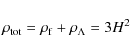
and
where
|
(3) |
and
|
(4) |
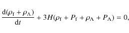
is the corresponding pressure. Also
and considering Eq. (1) we find:
where the over-dot denotes derivatives with respect to time. If the vacuum term is negligible,
Of course, in order to solve the above differential equation we need to
define explicitly the functional form of the
![]() component.
Note that the traditional
component.
Note that the traditional
![]() cosmology
can be described directly by the integration of the Eq. (6)
(for more details see Sect. 3.1).
cosmology
can be described directly by the integration of the Eq. (6)
(for more details see Sect. 3.1).
It is worth noting that the
![]() scenario has the caveat of its unknown exact
functional form, which however is also the case for the vast majority
of the dark energy models.
In the literature
there have been different phenomenological parametrizations which treat
the time-dependent
scenario has the caveat of its unknown exact
functional form, which however is also the case for the vast majority
of the dark energy models.
In the literature
there have been different phenomenological parametrizations which treat
the time-dependent
![]() function.
In particular, Freese et al. (1987) considered that
function.
In particular, Freese et al. (1987) considered that
![]() ,
with the constant c1 being the ratio of the
vacuum to the sum of vacuum and matter density (see
also Arcuri & Waga 1994). Chen & Wu (1990) proposed a different
ansatz in which
,
with the constant c1 being the ratio of the
vacuum to the sum of vacuum and matter density (see
also Arcuri & Waga 1994). Chen & Wu (1990) proposed a different
ansatz in which
![]() .
.
Recently, many authors (see for example
Ray et al. 2007; Sil & Som 2008, and references therein)
have investigated the global dynamical properties of the universe
considering that the vacuum energy density decreases linearly
either with the energy density or with the square Hubble parameter.
Attempts to provide a theoretical explanation for
the
![]() have also been presented in the
literature (see
Shapiro & Solá 2000; Babic et al. 2002;
Grande et al. 2006; Solá 2008, and references therein).
There it was found that a time dependent vacuum could
arise from the renormalization group (RG) in quantum field theory.
The corresponding solution for a running vacuum
is found to be
have also been presented in the
literature (see
Shapiro & Solá 2000; Babic et al. 2002;
Grande et al. 2006; Solá 2008, and references therein).
There it was found that a time dependent vacuum could
arise from the renormalization group (RG) in quantum field theory.
The corresponding solution for a running vacuum
is found to be
![]() (where c0
and c1 are constants; Grande et al. 2006)
and it can mimic the quintessence or phantom
behavior and a smooth transition between the two.
Alternatively, Schutzahold (2002) used
a different pattern in which the vacuum term is proportional to
the Hubble parameter,
(where c0
and c1 are constants; Grande et al. 2006)
and it can mimic the quintessence or phantom
behavior and a smooth transition between the two.
Alternatively, Schutzahold (2002) used
a different pattern in which the vacuum term is proportional to
the Hubble parameter,
![]() (see also Carneiro et al. 2008), while Basilakos (2009) considered
a power series form in H. Note that the
linear pattern,
(see also Carneiro et al. 2008), while Basilakos (2009) considered
a power series form in H. Note that the
linear pattern,
![]() ,
has been motivated theoretically
through a possible connection of cosmology with
the QCD scale of strong interactions (Schutzhold 2002).
In this context it has also been proposed that the
vacuum energy density can be defined from a possible link
of dark energy with QCD and
the topological structure of the universe (Urban & Zhitnitsky 2009a-c).
,
has been motivated theoretically
through a possible connection of cosmology with
the QCD scale of strong interactions (Schutzhold 2002).
In this context it has also been proposed that the
vacuum energy density can be defined from a possible link
of dark energy with QCD and
the topological structure of the universe (Urban & Zhitnitsky 2009a-c).
In this paper we have phenomenologically
identified a functional form of
![]() for which we can solve the main differential equation
(see Eq. (6)) analytically. This is:
for which we can solve the main differential equation
(see Eq. (6)) analytically. This is:
where the constants m and n are included for the consistency of units (see below). Although the above functional form was not motivated by some physical theory but rather phenomenologically by the fact that it provides analytical solutions to the Friedmann equation, its exact form can be physically justified a posteriori within the framework of the previously mentioned theoretical models (see Appendix A).
Using now Eq. (7), the generalized
Friedmann's equation (see Eq. (6)) becomes
and indeed, it is routine to perform the integration of Eq. (8) to obtain (see Appendix B):
![\begin{displaymath}
H(t)=\sqrt{n}{\rm e}^{mt}{\rm coth}\left[\frac{3(\beta+1-\gamma)\sqrt{n}}{2}S(t)\right]
\end{displaymath}](/articles/aa/full_html/2009/47/aa12575-09/img49.png)
where
while the range of values for which the above integration is valid is
![\begin{displaymath}a(t)=a_{1}
\sinh^{\frac{2}{3(\beta+1-\gamma)}}
\left[\frac{3(\beta+1-\gamma)\sqrt{n}}{2}S(t)\right] .
\end{displaymath}](/articles/aa/full_html/2009/47/aa12575-09/img53.png)
The relevant units of
where
In this context, the density of the cosmic fluid evolves with
time (see Eq. (1)) as:
|
(13) |
or
In the following sections, we investigate thoroughly whether such a generalized vacuum component in an expanding universe allows for a late accelerated phase of the universe, and under which circumstances such an approach provides a viable solution to the fine-tuning problem as well as to the cosmic coincidence problem.
3 The matter+vacuum scenario
In a matter+vacuum expanding universe
(
![]() ), we attempt to investigate
the correspondence of the
), we attempt to investigate
the correspondence of the
![]() pattern with the traditional
pattern with the traditional
![]() -cosmology in order to show
the extent to which they compare. In particular,
we will prove that the Hubble expansion, provided
by the current time-dependent vacuum, is
a generalization of the traditional
-cosmology in order to show
the extent to which they compare. In particular,
we will prove that the Hubble expansion, provided
by the current time-dependent vacuum, is
a generalization of the traditional ![]() cosmology.
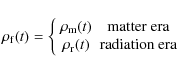
Note that in the present formalism the matter era
corresponds to
cosmology.
Note that in the present formalism the matter era
corresponds to ![]() .
.
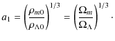
3.1 The standard  -cosmology
Let us first investigate the solution for
Now, using the well know parametrization
the scale factor of the universe is given by
where (see Eq. (12))
The cosmic time is related with the scale factor as
|
(19) |
Combining the above equations we can define the Hubble expansion as a function of the scale factor:
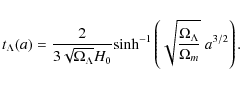
In principle, H0 and
![$\displaystyle t_{I\Lambda}=\frac{2}{3\sqrt{\Omega_{\Lambda}}H_{0}}
{\rm sinh^{-...
...\;\;
a_{I\Lambda}=\left[\frac{\Omega_{m}}{2\Omega_{\Lambda}}\right]^{1/3} \cdot$](/articles/aa/full_html/2009/47/aa12575-09/img74.png)
Therefore, we estimate
Finally, due to the fact that the traditional ![]() cosmology
is a particular solution
of the current time varying vacuum models with
cosmology
is a particular solution
of the current time varying vacuum models with
![]() strictly equal to (0,0),
the constant value n is always
defined by Eq. (16). That is why
all relevant cosmological quantities are parametrized according to
strictly equal to (0,0),
the constant value n is always
defined by Eq. (16). That is why
all relevant cosmological quantities are parametrized according to
![]() throughout the paper.
throughout the paper.
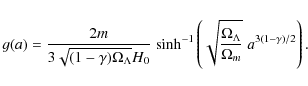
3.2 ``The general'' (t) model
In this section, we examine a more general class of vacuum models with
![\begin{displaymath}
H(t)=\sqrt{\Omega_{\Lambda}}\;H_{0}\;{\rm e}^{mt}{\rm coth}
...
...amma)\sqrt{\Omega_{\Lambda}}H_{0}}{2m}({\rm e}^{mt}-1)\right]
\end{displaymath}](/articles/aa/full_html/2009/47/aa12575-09/img80.png)
and
![\begin{displaymath}a(t)=a_{1}
\sinh^{\frac{2}{3(1-\gamma)}}
\left[\frac{3(1-\gamma)\sqrt{\Omega_{\Lambda}}H_{0}}{2m}({\rm e}^{mt}-1) \right]
\end{displaymath}](/articles/aa/full_html/2009/47/aa12575-09/img81.png)
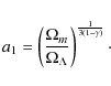
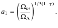
or
![\begin{displaymath}t(a)=\frac{1}{m}{\rm ln}\left[1+\frac{2m}{3(1-\gamma)\sqrt{\O...
...nh^{-1}}\left(\frac{a}{a_{1}}\right)^{3(1-\gamma)/2} \right] .
\end{displaymath}](/articles/aa/full_html/2009/47/aa12575-09/img82.png)
Obviously, if
|
(25) |
Taking the above expressions into account, the basic cosmological quantities as a function of the scale factor become
![\begin{displaymath}H(a)=H_{0}\left[1+g(a)\right]\left[\Omega_{\Lambda}+\Omega_{m}a^{-3(1-\gamma)}\right]^{1/2}
\end{displaymath}](/articles/aa/full_html/2009/47/aa12575-09/img86.png)
|
(26) |
and
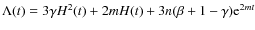
![\begin{displaymath}\Lambda_{\gamma m}(a)=3\gamma H^{2}+2mH+3H^{2}_{0}\Omega_{\Lambda}(1-\gamma)[1+g(a)]^{2}
\end{displaymath}](/articles/aa/full_html/2009/47/aa12575-09/img87.png)
where
|
(28) |
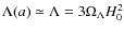
If we take
![\begin{displaymath}H(a)=\left[1+g(a)\right]H_{\Lambda}(a)
\end{displaymath}](/articles/aa/full_html/2009/47/aa12575-09/img90.png)
|
(29) |
which means that as long as the function g(a) takes small values (
![\begin{displaymath}
\Lambda_{0m}(a)=2mH(a)+3H^{2}_{0}\Omega_{\Lambda}[1+g(a)]^{2} .
\end{displaymath}](/articles/aa/full_html/2009/47/aa12575-09/img93.png)
Finally, the fact that the vacuum term has units of
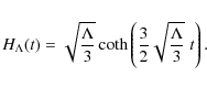
3.3 ``The modified'' model
Now we consider
![\begin{displaymath}
H(t)=\sqrt{\Omega_{\Lambda}}\;H_{0}
\;{\rm coth}\left[\frac{3(1-\gamma)\sqrt{\Omega_{\Lambda}}H_{0}}{2}\;t\right] .
\end{displaymath}](/articles/aa/full_html/2009/47/aa12575-09/img98.png)
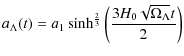
Using now Eqs. ((10), (11)), the scale factor of the universe a(t) evolves with time as
![\begin{displaymath}a(t)=a_{1}
\sinh^{\frac{2}{3(1-\gamma)}}
\left[\frac{3(1-\gamma)\sqrt{\Omega_{\Lambda}}H_{0}}{2}\;t\right]
\end{displaymath}](/articles/aa/full_html/2009/47/aa12575-09/img99.png)
where
Inverting Eq. (32) we estimate the cosmic time:
The corresponding inflection point (
or
![\begin{displaymath}a_{I}=\left[\frac{(1-3\gamma)\Omega_{m}}{2\Omega_{\Lambda}}\right]^{1/3(1-\gamma)}
\end{displaymath}](/articles/aa/full_html/2009/47/aa12575-09/img104.png)
|
(36) |
which implies that the condition for which an inflection point is present in the evolution of the scale factor is
As expected, for
![]() the
above solution tends to the concordance model,
the
above solution tends to the concordance model,
![]() .
Now from Eqs. ((31), (32)), using the well known
hyperbolic formula
.
Now from Eqs. ((31), (32)), using the well known
hyperbolic formula
![]() ,
we arrive
after some algebra:
,
we arrive
after some algebra:
![\begin{displaymath}H(a)=H_{0}\left[\Omega_{\Lambda}+\Omega_{m}a^{-3(1-\gamma)}\right]^{1/2} .
\end{displaymath}](/articles/aa/full_html/2009/47/aa12575-09/img109.png)
|
(37) |
From this analysis it becomes clear that the Hubble expansion predicted by the
As we have previously mentioned in Sect. 2, the above phenomenological functional form (see Eq. (38)) is motivated theoretically by the renormalization group (RG) in the quantum field theory (Shapiro & Solá 2000; Babic et al. 2002; Solá 2008). Moreover, recent studies (see Grande et al. 2006; and Grande et al. 2009) find that this solution alleviates the cosmic coincidence problem (see Sect. 5.1). Obviously, at late enough times (
4 The radiation+vacuum scenario
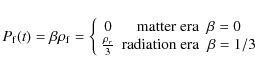
In this section, we consider a universe that is spatially flat but contains both radiation and a time vacuum term. This crucial period in the cosmic history corresponds to
where,
- radiation+constant vacuum:
 :
The scale factor is
:
The scale factor is
(39)
Owing to the fact that in this period ,
the above solution reduces to the
following simple analytic approximation:
,
the above solution reduces to the
following simple analytic approximation:
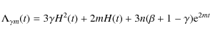
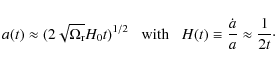
- radiation+general vacuum:
 :
this general scenario provides
:
this general scenario provides
![\begin{displaymath}a(t)=\left(\frac{\Omega_{\rm r}}{\Omega_{\Lambda}}\right)^{\f...
...ma_{1}\sqrt{\Omega_{\Lambda}}H_{0}}{m}({\rm e}^{mt}-1) \right]
\end{displaymath}](/articles/aa/full_html/2009/47/aa12575-09/img120.png)
(41)
where .
The vacuum component as a function of time (see Eq. (7)) is
.
The vacuum component as a function of time (see Eq. (7)) is
or
It is very interesting that during the radiation epoch .
For small values
of
.
For small values
of  or
or
 ,
the latter relation
implies that as long as the scale factor tends to zero the
vacuum term moves rapidly to infinity
(see Sect. 6).
In the case of
,
the latter relation
implies that as long as the scale factor tends to zero the
vacuum term moves rapidly to infinity
(see Sect. 6).
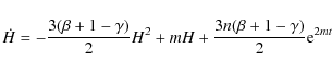
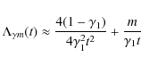
In the case of
 (or
(or
 ), the vacuum term
(see Eqs. (42) and (43))
varies with time as
), the vacuum term
(see Eqs. (42) and (43))
varies with time as
(44)
Now the vacuum component evolves as ,
in agreement with the Chen & Wu (1990) model.
,
in agreement with the Chen & Wu (1990) model.
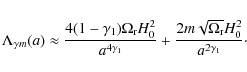
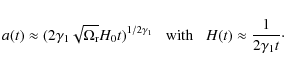
- radiation+modified vacuum:
 ,
,
 :
in this cosmological model we have
:
in this cosmological model we have
![\begin{displaymath}a(t)=\left(\frac{\Omega_{\rm r}}{\Omega_{\Lambda}}\right)^{\f...
...{1}}}
\left[2\gamma_{1}\sqrt{\Omega_{\Lambda}}H_{0}\;t \right]
\end{displaymath}](/articles/aa/full_html/2009/47/aa12575-09/img130.png)
(45)
where.
The approximate solution now becomes
The vacuum component (see Eq. (7)) evolves with time as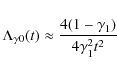
(47)
or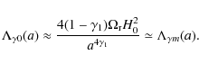
(48)
Obviously, for (
)
the vacuum energy density
goes rapidly to infinity.
(
)
the vacuum energy density
goes rapidly to infinity.
5 Tackling the cosmological puzzles
As we have stated already in the introduction, there is a possibility
for the vacuum energy to be a function of time
rather than having a constant value. Therefore, in this section
we compare the cosmic phases of the
![]() scenarios (described in the previous sections)
and the concordance
scenarios (described in the previous sections)
and the concordance ![]() -cosmology.
The aim here is to investigate the consequences
of such a comparison on the basic cosmological puzzles,
namely the cosmic coincidence problem and fine-tuning problem.
-cosmology.
The aim here is to investigate the consequences
of such a comparison on the basic cosmological puzzles,
namely the cosmic coincidence problem and fine-tuning problem.
5.1 The coincidence problem
In order to investigate the coincidence problem we
define the time-dependent proximity parameter of
![]() (see Eq. (14)) and
(see Eq. (14)) and
![]() (see Egan & Lineweaver 2008, and references therein):
(see Egan & Lineweaver 2008, and references therein):
![\begin{displaymath}
r(a)\equiv {\rm min}\left[\frac{\rho_{\Lambda}(a)}{\rho_{m}(a)},
\frac{\rho_{m}(a)}{\rho_{\Lambda}(a)} \right]
\end{displaymath}](/articles/aa/full_html/2009/47/aa12575-09/img138.png)
where in this work we use
In particular,
suppose that we have a cosmological model which
accommodates a late time accelerated expansion and
contains n-free parameters, described by the vector
![]() .
The main question that we should address here is the following:
``what is the range of input
.
The main question that we should address here is the following:
``what is the range of input
![]() parameters for which the coincidence problem
can be avoided?'' Below we implement the following tests.
parameters for which the coincidence problem
can be avoided?'' Below we implement the following tests.
- (i)
- We find the range of the free parameters of the considered
cosmological model that implies
 for at least two different
epochs, one of which is precisely the present epoch.
for at least two different
epochs, one of which is precisely the present epoch.
- (ii)
- We know that for epochs between the inflection point and the
present time
 ,
the proximity parameter is
,
the proximity parameter is
 .
As an example, for the traditional -cosmology we
have
.
As an example, for the traditional -cosmology we
have
 .
Thus, the goal here is to define the range of the
free parameters in which at least a second region
with
.
Thus, the goal here is to define the range of the
free parameters in which at least a second region
with
 occurs before the inflection point (a<aI).
![\begin{displaymath}
\chi^{2}({\vec \epsilon})=\sum_{j=1}^{307} \left[ \frac{ {\c...
...)-{\cal \mu}^{\rm obs}(a_{j}) }
{\sigma_{j}} \right]^{2} \cdot
\end{displaymath}](/articles/aa/full_html/2009/47/aa12575-09/img153.png)
where aj=(1+zj)-1 is the observed scale factor of the universe, zj is the observed redshift,
|
(51) |
where
A cosmological model for which the present tests are successfully passed
should not suffer from the coincidence problem.
Below we apply our tests
to the current
![]() cosmological models (see also Table 1).
cosmological models (see also Table 1).
- The modified vacuum model with
 :
We sample the unknown parameter as follows:
:
We sample the unknown parameter as follows:
 in steps of 10-4.
We confirm that in the range of
in steps of 10-4.
We confirm that in the range of
![$\gamma \in [0.004,0.03]$](/articles/aa/full_html/2009/47/aa12575-09/img162.png) the
the
 model
model![[*]](/icons/foot_motif.png) satisfies both the criteria (i); and
(ii) respectively. Also, we verify that this range of values fits
the SnIa data,
satisfies both the criteria (i); and
(ii) respectively. Also, we verify that this range of values fits
the SnIa data,
 very well. Notice that for
 the criterion (i) is not satisfied.
As an example, in the upper panel of Fig. 1 we present
the evolution of the proximity parameter
for
the criterion (i) is not satisfied.
As an example, in the upper panel of Fig. 1 we present
the evolution of the proximity parameter
for
 (solid line) and 0.03 (dashed line).
It becomes clear is that
for
(solid line) and 0.03 (dashed line).
It becomes clear is that
for
 (or
(or
 )
the vacuum density
is low enough (
)
the vacuum density
is low enough ( )
to allow galaxies and galaxy clusters to
form (Garriga et al. 1999; Basilakos et al. 2009).
From now on, we will utilize
)
to allow galaxies and galaxy clusters to
form (Garriga et al. 1999; Basilakos et al. 2009).
From now on, we will utilize
 that corresponds to the best
fit parameter. Thus it becomes clear that
the
model passes the above criteria and
does not suffer from the cosmic coincidence problem.
that corresponds to the best
fit parameter. Thus it becomes clear that
the
model passes the above criteria and
does not suffer from the cosmic coincidence problem.
- The mild vacuum model with
 :
In this cosmological model we find that for
:
In this cosmological model we find that for
 ,
the corresponding age of the universe is
,
the corresponding age of the universe is
 Gyr. The latter
appears to be ruled out by the ages of the oldest
known globular clusters (Krauss 2003; Hansen et al. 2004).
Using this constraint the unknown m parameter
has an upper limit of 0.17H0, and we perform the
following sampling:
Gyr. The latter
appears to be ruled out by the ages of the oldest
known globular clusters (Krauss 2003; Hansen et al. 2004).
Using this constraint the unknown m parameter
has an upper limit of 0.17H0, and we perform the
following sampling:
 in steps of
 .
Within this range,
we find that the required (i) and (ii) criteria are not satisfied.
Thus, the
.
Within this range,
we find that the required (i) and (ii) criteria are not satisfied.
Thus, the
 cosmological model suffers from the
coincidence problem. The resulting minimization provides:
cosmological model suffers from the
coincidence problem. The resulting minimization provides:
 with
.
Note that the errors of the fitted
parameters represent
with
.
Note that the errors of the fitted
parameters represent  uncertainties.
- The general vacuum model with
 :
This vacuum cosmological model contains 2 free parameters. Using
the sampling mentioned previously, we obtain that
our main criteria for the
:
This vacuum cosmological model contains 2 free parameters. Using
the sampling mentioned previously, we obtain that
our main criteria for the
 scenario are fullfilled for
![$\gamma \in [0.004,0.02]$](/articles/aa/full_html/2009/47/aa12575-09/img181.png) ,
,
![$m \in [1.4\times 10^{-3}H_{0},9\times 10^{-3}H_{0}]$](/articles/aa/full_html/2009/47/aa12575-09/img182.png) with
with
![$\chi^{2}_{\rm min}/{\rm d.o.f.}\in [1.01,1.02]$](/articles/aa/full_html/2009/47/aa12575-09/img183.png) .
Throughout the rest of the paper we will use the best fit parameters. These are:
.
Throughout the rest of the paper we will use the best fit parameters. These are:
 and
and
![\begin{figure}
\par\includegraphics[angle=0,scale=0.45]{12575fg1.eps} \vspace{-3mm}
\end{figure}](/articles/aa/full_html/2009/47/aa12575-09/img187.png)
|
Figure 1:
Upper panel: the evolution of the proximity parameter
for the
|
| Open with DEXTER | |
Table 1: Numerical results.
5.2 The cosmic evolution - fine-tuning problem
Using now our best fit parameters for the different kind of vacuums, we present in Fig. 1 the corresponding normalized energy densities, vacuumIn particular, for the
![]() vacuum scenario (the same behavior holds for
vacuum scenario (the same behavior holds for
![]() )
we have revealed the following phases:
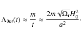
(a) at early enough times (
)
we have revealed the following phases:
(a) at early enough times (
![]() )
the scale factor of the
universe tends to its minimum value,
)
the scale factor of the
universe tends to its minimum value,
![]() ,
which means that the vacuum energy density
initially moves quickly to infinity.
So, as long as the scale factor increases
the vacuum energy rolls down rapidly as
,
which means that the vacuum energy density
initially moves quickly to infinity.
So, as long as the scale factor increases
the vacuum energy rolls down rapidly as
![]() (where
(where
![]() ).
This evolution may solve the fine-tuning problem. Indeed,
for
).
This evolution may solve the fine-tuning problem. Indeed,
for
![]() ,
we find that prior to the inflation point
(
,
we find that prior to the inflation point
(
![]() s), the vacuum energy density
divided by its present value is
s), the vacuum energy density
divided by its present value is
![]() Finally, if we consider that the functional form of
Finally, if we consider that the functional form of
![]() is still valid during the
Planck time (
is still valid during the
Planck time (
![]() s), then
s), then
![]() (see the last rows in Table 1); and (b) in the matter era the vacuum density
continues to roll down but with a
different power law
(see the last rows in Table 1); and (b) in the matter era the vacuum density
continues to roll down but with a
different power law
![]() and it tends to a constant value
close to
and it tends to a constant value
close to
![]() (
(![]() ). Finally,
for
). Finally,
for ![]() the vacuum energy density is effectively frozen to
the nominal value,
the vacuum energy density is effectively frozen to
the nominal value,
![]() ,
which implies that the considered time varying vacuum model explains
why the matter energy density and the dark energy density are of the same
order prior to the present epoch.
The moment of radiation-vacuum equality occurs at
,
which implies that the considered time varying vacuum model explains
why the matter energy density and the dark energy density are of the same
order prior to the present epoch.
The moment of radiation-vacuum equality occurs at
![]() .
Similarly, the moment of matter-vacuum equality takes place at
.
Similarly, the moment of matter-vacuum equality takes place at
![]() .
From the observational viewpoint,
in order to investigate whether the vacuum
energy density follows the above evolution, we need a robust
cosmological probe at redshifts
.
From the observational viewpoint,
in order to investigate whether the vacuum
energy density follows the above evolution, we need a robust
cosmological probe at redshifts ![]() .
In a recent paper (Basilakos et al. 2009) we have investigated
how realistic it would be to detect differences among the vacuum models.
In particular, we have found that the Sunayev-Zeldovich cluster
number-counts (as expected from the survey of the South Pole
Telescope, Staniszewski et al. 2009, and the Atacama Cosmology
Telescope, Hincks et al. 2009)
indicate that we may be able to detect significant
differences among the vacuum models in the redshift range
.
In a recent paper (Basilakos et al. 2009) we have investigated
how realistic it would be to detect differences among the vacuum models.
In particular, we have found that the Sunayev-Zeldovich cluster
number-counts (as expected from the survey of the South Pole
Telescope, Staniszewski et al. 2009, and the Atacama Cosmology
Telescope, Hincks et al. 2009)
indicate that we may be able to detect significant
differences among the vacuum models in the redshift range
![]() at a level of
at a level of ![]()
![]() ,
which translates in number count
differences over the whole sky of
,
which translates in number count
differences over the whole sky of ![]() 100 clusters
(see Fig. 6 in Basilakos et al. 2009).
100 clusters
(see Fig. 6 in Basilakos et al. 2009).
![\begin{figure}
\par\includegraphics[angle=0,scale=0.4]{12575fg2.eps}\vspace{-3mm}
\end{figure}](/articles/aa/full_html/2009/47/aa12575-09/img222.png)
|
Figure 2:
Upper panel:
comparison of the scale factor provided by our
|
| Open with DEXTER | |
Finally, in Fig. 1 we also show the evolution of the
mild vacuum model
![]() (dot line), in which
(dot line), in which ![]() .
Briefly, we get the following dependence:
(a)
.
Briefly, we get the following dependence:
(a)
![]() for
for
![]() ,
while we estimate that
,
while we estimate that
![]() and
and
![]() ;
(b) between
;
(b) between
![]() we have
we have
![]() ;
and (c)
for
;
and (c)
for ![]() the
the
![]() becomes constant.
becomes constant.
We would like to end this section with a
discussion of the evolution of the scale factor.
In particular, our approach provides an evolution of the
scale factor in the
![]() model seen in the upper panel of Fig. 2 as the solid line,
which mimics the corresponding scale factor of the
model seen in the upper panel of Fig. 2 as the solid line,
which mimics the corresponding scale factor of the ![]() cosmological model (open points), despite the
fact that they describe the vacuum term
differently.
On the other hand, in the bottom panel of
Fig. 2 we present the corresponding deviation
cosmological model (open points), despite the
fact that they describe the vacuum term
differently.
On the other hand, in the bottom panel of
Fig. 2 we present the corresponding deviation
![]() ,
of the growth factors.
It becomes evident that within the range
0 < H0t< 5
the evolution of the
scale factor provided by the
,
of the growth factors.
It becomes evident that within the range
0 < H0t< 5
the evolution of the
scale factor provided by the
![]() model
closely resembles, the corresponding scale factor of the
model
closely resembles, the corresponding scale factor of the
![]() model
(the same result holds also for the
model
(the same result holds also for the ![]() cosmology).
However, for models where
cosmology).
However, for models where ![]() the situation is somewhat different in the far future.
Indeed, for
the situation is somewhat different in the far future.
Indeed, for
![]() the
the
![]() (or
(or
![]() )
cosmological scenario
deviates from the
)
cosmological scenario
deviates from the
![]() (or
(or ![]() )
model by
)
model by
![]()
![]() .
Thus, we conclude that the
models with
.
Thus, we conclude that the
models with ![]() give a super-accelerated expansion of the
universe in the far future with respect to those vacuum models where m=0.
give a super-accelerated expansion of the
universe in the far future with respect to those vacuum models where m=0.
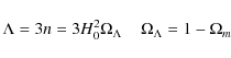
6 Conclusions
The reason why a cosmological constant leads to a late cosmic acceleration is because it introduces in Friedmann's equation a component which has an equation of state with negative pressure,Below we wish to present the basic assumptions and conclusions of our analysis.
- We are assuming a time varying vacuum pattern in which
the specific functional form is:
 ,
where
,
where  (matter era) or
  (radiation era),
 ,
while the pair
,
while the pair
 characterizes the different types of vacuum. Note
that the above functional form includes the effect of the quantum
field theory (for m=0) (Shapiro & Solá 2000;
Babic et al. 2002;
Grande et al. 2006; Solá 2008) and it also extents recent studies
(see for example Ray et al. 2007; Carneiro et al. 2008;
Sil & Som 2008; Basilakos 2009). In this context
we can easily prove that the cosmological constant is
a particular solution of the general vacuum, that
.
We have also investigated the following models: (a) modified vacuum in
which
,
mild vacuum with
and
general vacuum in which
.
In this framework we find that the time evolution of the basic cosmological
functions (scale factor and Hubble flow) is described in terms of
hyperbolic functions which can accommodate a late time accelerated
expansion equivalent to the standard model.
characterizes the different types of vacuum. Note
that the above functional form includes the effect of the quantum
field theory (for m=0) (Shapiro & Solá 2000;
Babic et al. 2002;
Grande et al. 2006; Solá 2008) and it also extents recent studies
(see for example Ray et al. 2007; Carneiro et al. 2008;
Sil & Som 2008; Basilakos 2009). In this context
we can easily prove that the cosmological constant is
a particular solution of the general vacuum, that
.
We have also investigated the following models: (a) modified vacuum in
which
,
mild vacuum with
and
general vacuum in which
.
In this framework we find that the time evolution of the basic cosmological
functions (scale factor and Hubble flow) is described in terms of
hyperbolic functions which can accommodate a late time accelerated
expansion equivalent to the standard model.
- We find that within the framework of either the
modified or general vacuum models the corresponding vacuum term in the
radiation era varies as
 while in the
matter-dominated era
we have
while in the
matter-dominated era
we have
 up to
up to
 while
while
 for
for  .
This vacuum mechanism simultaneously
sets (a) the value of
at the present time to its
observed value; and (b) at the Planck time to a value which is
10124 at its present value
(
.
This vacuum mechanism simultaneously
sets (a) the value of
at the present time to its
observed value; and (b) at the Planck time to a value which is
10124 at its present value
(
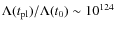 ).
Additionally, we verify that our models appear to overcome
the cosmic coincidence problem.
Finally, in order to
confirm the above results, we need to define a robust
cosmological probe at high redshifts (
).
Additionally, we verify that our models appear to overcome
the cosmic coincidence problem.
Finally, in order to
confirm the above results, we need to define a robust
cosmological probe at high redshifts ( ).
In Basilakos
et al. (2009) we propose that the future
cluster surveys based on the Sunayev-Zeldovich
detection method will possibly distinguish the closely resembling
vacuum models at high redshifts.
).
In Basilakos
et al. (2009) we propose that the future
cluster surveys based on the Sunayev-Zeldovich
detection method will possibly distinguish the closely resembling
vacuum models at high redshifts.
I would like to thank the anonymous referee for his/her useful comments and suggestions.
Appendix A
In this appendix we provide a physical justification of the functional form ofAll the above options have merits and demerits.
In the current paper the functional form of
![]() is motivated by a combination
of the above possibilities, namely
H2(t) [RG], H(t) [QCD] and
is motivated by a combination
of the above possibilities, namely
H2(t) [RG], H(t) [QCD] and
![]() (dark energy).
In particular, the linear combination reads as follows:
(dark energy).
In particular, the linear combination reads as follows:

which obviously is very similar to the original (phenomenologically selected) form of
Appendix B
With the aid of the differential equation theory we present solutions that are relevant to our Eq. (8). If we have a Riccati differential equation which is given by the following special form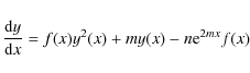
then the general solution of Eq. (52) for n>0 is
![\begin{displaymath}y(x)=\sqrt{n}{\rm e}^{mx}{\rm coth}\left[-\sqrt{n}\int_{x_{0}}^{x}
{\rm e}^{mu}f(u){\rm d}u \right] .
\end{displaymath}](/articles/aa/full_html/2009/47/aa12575-09/img248.png)
|
(53) |
On the other hand, if n<0 then the solution of Eq. (52) is
![\begin{displaymath}y(x)=\sqrt{\vert n\vert}{\rm e}^{mx}{\rm cot}\left[-\sqrt{\vert n\vert}\int_{x_{0}}^{x}
{\rm e}^{mu}f(u){\rm d}u \right] .
\end{displaymath}](/articles/aa/full_html/2009/47/aa12575-09/img249.png)
|
(54) |
Note that in our formulation the function f(x) is a constant:
References
- Alcaniz, J. S., & Lima, J. A. S. 2005, Phys. Rev. D, 72, 063516 [NASA ADS] [CrossRef]
- Amendola, L., Quercellini, C., Tocchini-Valentini, D., & Pasqui, A. 2003, ApJ, 583, L53 [NASA ADS] [CrossRef]
- Arcuri, R. C., & Waga., I. 1994, Phys. Rev. D, 50, 2928 [NASA ADS] [CrossRef]
- Babic, A., Guberina, B., Horvat, R., & Stefancic, H. 2002, Phys. Rev. D, 65, 085002 [NASA ADS] [CrossRef]
- Basilakos, S. 2009, MNRAS, 395, 2347 [NASA ADS] [CrossRef]
- Basilakos, S., Plionis, M., & Solá, J. 2009, Phys. Rev. D, 80, 083511 [CrossRef]
- Barrow, J. D., & Clifton, T. 2006, Phys. Rev. D, 73, 103520 [NASA ADS] [CrossRef]
- Bauer, F. 2005, Class. Quant. Grav., 22, 3533 [NASA ADS] [CrossRef]
- Bertolami, O. 1986, Nuovo Cimento B, 93, 36 [NASA ADS] [CrossRef]
- Bertolami, O., & Martins, P. J. 2000, Phys. Rev. D, 61, 064007 [NASA ADS] [CrossRef]
- Binder, J. B., & Kremer, G. M. 2006, Gen. Rel. Grav. 38, 857
- Cai, R. G., & Wang, A. 2005, JCAP, 0503, 002 [NASA ADS]
- Caldwell, R. R., Dave, R., & Steinhardt, P. J. 1998, Phys. Rev. Lett., 80, 1582 [NASA ADS] [CrossRef]
- Carneiro, S., Dantas, M. A., Pigozzo, C., & Alcaniz, J. S. 2008, Phys. Rev. D, 77, 3504 [CrossRef]
- Carvalho, J. C., Lima, J. A. S., & Waga, I. 1992, Phys. Rev. D, 46, 2404 [NASA ADS] [CrossRef]
- Chen, Wei, & Wu, Yong-Shi 1990, Phys. Rev. D, 41, 695 [NASA ADS] [CrossRef]
- Davis, T. M., Mörtsell, E., Sollerman, J., et al. 2007, ApJ, 666, 716 [NASA ADS] [CrossRef]
- Das, S., Corasaniti, P. S., & Khoury, J. 2006, Phys. Rev. D, 73, 083509 [NASA ADS] [CrossRef]
- Egan, C. A., & Lineweaver, C. H. 2008, Phys. Rev. D, 78, 3528 [CrossRef]
- Eisenstein, D. J., Zehavi, I., Hogg, D. W., et al. 2005, ApJ, 633, 560 [NASA ADS] [CrossRef]
- Freese, K., Adams, F. C., Frieman, J. A., & Mottola, E. 1987, Nucl. Phys., 287, 797 [NASA ADS] [CrossRef]
- Hansen, B., Richer, H. B., Fahlman, G. G., et al. 2004, ApJS, 155, 551 [NASA ADS] [CrossRef]
- Hincks, A. D., et al. 2009, ApJ, submitted [arXiv.0907.0461]
- Garriga, J., M. Livio, M., & Vilenkin, A. 1999, Phys. Rev. D, 61, 023503 [NASA ADS] [CrossRef]
- Grande, J., Solá, J., & Stefancic, H. 2006, JCAP, 8, 11 [NASA ADS]
- Grande, J., Pelinson A., & Solá, J. 2009, Phys. Rev. D, 79, 043006 [NASA ADS] [CrossRef]
- Komatsu, E., Dunkley, J., Nolta, M. R., et al. 2009, ApJS, 180, 330 [NASA ADS] [CrossRef]
- Kowalski, M., Rubin, D., Aldering, G., et al. 2008, ApJ, 686, 749 [NASA ADS] [CrossRef]
- Krauss, L. M. 2003, ApJ, 596, L1 [NASA ADS] [CrossRef]
- Montenegro, Jr., & Carneiro, S. 2007, Class. Quant. Grav., 24, 313 [NASA ADS] [CrossRef]
- Olivares, G., Atrio-Barandela, F., & Pavón, D. 2008, Phys. Rev. D, 77, 063513 [NASA ADS] [CrossRef]
- Overduin J. M., & Cooperstock, F. I. 1998, Phys. Rev. D, 58, 043506 [NASA ADS] [CrossRef]
- Opher, R., & Pellison, A. 2004, Phys. Rev. D, 70, 063529 [NASA ADS] [CrossRef]
- Ozer, M., & Taha, O. 1987, Nucl. Phys. B, 287, 776 [NASA ADS] [CrossRef]
- Peebles, P. J. E., & Ratra, B. 1988, ApJ, 325, L17 [NASA ADS] [CrossRef]
- Peebles, P. J. E., & Ratra, B. 2003, Rev. Mod. Phys., 75, 559 [NASA ADS] [CrossRef]
- Ratra, B., & Peebles, P. J. E. 1988, Phys. Rev. D, 37, 3406 [NASA ADS] [CrossRef]
- Padmanabhan, T. 2003, Phys. Rept., 380, 235 [NASA ADS] [CrossRef]
- Padmanabhan, N., Schlegel, D. J., Seljak, U., et al. 2007, MNRAS, 378, 852 [NASA ADS] [CrossRef]
- Perivolaropoulos, L. 2008 [arXiv.0811.4684]
- Ray, S., Mukhopadhyay, U., & Meng, Xin-He 2007, Grav. Cosmol., 13, 142 [NASA ADS]
- Shapiro, I. L., & Solá, J. 2000, Phys. Lett. B, 475, 236 [NASA ADS] [CrossRef]
- Sil, A., & Som, S. 2008, Ap&SS, 318, 109 [NASA ADS] [CrossRef]
- Solá, J. 2008, JPhA, 41, 4066 [NASA ADS]
- Spergel, D. N., Bean, R., Doré, O., et al. 2007, ApJS, 170, 377 [NASA ADS] [CrossRef]
- Schutzhold, R. 2002, Phys. Rev. D, 89, 081302
- Staniszewski, Z., Ade, P. A. R., Aird, K. A., et al. 2009, ApJ, 701, 32 [NASA ADS] [CrossRef]
- Tegmark, M., Blanton, M. R., Strauss, M. A., et al. 2004, ApJ, 606, 702 [NASA ADS] [CrossRef]
- Turner, M. S., & White, M. 1997, Phys. Rev. D, 56, 4439 [NASA ADS] [CrossRef]
- Urban, F. R., & Zhitnitsky, A. R. 2009a [arXiv:0906.2162]
- Urban, F. R., & Zhitnitsky, A. R. 2009b, Phys. Rev. D, 80, 063001 [NASA ADS] [CrossRef]
- Urban F. R., & Zhitnitsky, A. R. 2009c, JCAP, 09, 18 [NASA ADS]
- Wang P., & Meng, X. 2005, Clas. Quant. Grav., 22, 283 [NASA ADS] [CrossRef]
- Weinberg, S. 1989, Rev. Mod. Phys., 61, 1 [NASA ADS] [CrossRef]
- Zimdahl, W., Pavón, D., & Chimento, L. P. 2001, Phys. Lett. B, 521, 133 [NASA ADS] [CrossRef]
Footnotes
- ... model
- Note that from a theoretical
viewpoint the predicted value of the parameter is
 ,
where
,
where  is the Planck mass and M is an effective mass
parameter representing the average mass of the heavy particles of
the Grand Unified Theory (GUT) near the Planck scale, after taking
into account their multiplicities. In the case of
is the Planck mass and M is an effective mass
parameter representing the average mass of the heavy particles of
the Grand Unified Theory (GUT) near the Planck scale, after taking
into account their multiplicities. In the case of
 we can derive an upper limit of
 (for more details see Basilakos et al. 2009).
All Tables
Table 1: Numerical results.
All Figures
|
|
Figure 1:
Upper panel: the evolution of the proximity parameter
for the
|
| Open with DEXTER | |
| In the text | |
|
|
Figure 2:
Upper panel:
comparison of the scale factor provided by our
|
| Open with DEXTER | |
| In the text | |
Copyright ESO 2009
Current usage metrics show cumulative count of Article Views (full-text article views including HTML views, PDF and ePub downloads, according to the available data) and Abstracts Views on Vision4Press platform.
Data correspond to usage on the plateform after 2015. The current usage metrics is available 48-96 hours after online publication and is updated daily on week days.
Initial download of the metrics may take a while.