Wave propagation and energy transport in the magnetic network of the Sun

G. Vigeesh; S. S. Hasan; O. Steiner

doi:10.1051/0004-6361/200912450

Home

All issues

Volume 508 / No 2 (December III 2009)

A&A, 508 2 (2009) 951-962

Full HTML

Free Access

Issue		A&A Volume 508, Number 2, December III 2009


Page(s)		951 - 962
Section		The Sun
DOI		https://doi.org/10.1051/0004-6361/200912450
Published online		15 September 2009

A&A 508, 951-962 (2009)

Wave propagation and energy transport in the magnetic network of the Sun

G. Vigeesh^1,2 - S. S. Hasan¹ - O. Steiner²

1 - Indian Institute of Astrophysics, Block II Koramangala, Bangalore-560034, India
2 - Kiepenheuer-Institut für Sonnenphysik, Schöneckstrasse 6, 79104 Freiburg, Germany

Received 8 May 2009 / Accepted 10 September 2009

Abstract
Aims. We investigate wave propagation and energy transport in magnetic elements, which are representatives of small scale magnetic flux concentrations in the magnetic network on the Sun. This is a continuation of earlier work by Hasan et al. (2005, ApJ, 631, 1270). The new features in the present investigation include a quantitative evaluation of the energy transport in the various modes and for different field strengths, as well as the effect of the boundary-layer thickness on wave propagation.
Methods. We carry out 2D MHD numerical simulations of magnetic flux concentrations for strong and moderate magnetic fields for which $\beta$ (the ratio of gas to magnetic pressure) on the tube axis at the photospheric base is 0.4 and 1.7, respectively. Waves are excited in the tube and ambient medium by a transverse impulsive motion of the lower boundary.
Results. The nature of the modes excited depends on the value of $\beta$ . Mode conversion occurs in the moderate field case when the fast mode crosses the $\beta =1$ contour. In the strong field case the fast mode undergoes conversion from predominantly magnetic to predominantly acoustic when waves are leaking from the interior of the flux concentration to the ambient medium. We also estimate the energy fluxes in the acoustic and magnetic modes and find that in the strong field case, the vertically directed acoustic wave fluxes reach spatially averaged, temporal maximum values of a few times 10⁶ erg cm^-2 s^-1 at chromospheric height levels.
Conclusions. The main conclusions of our work are twofold: firstly, for transverse, impulsive excitation, flux tubes/sheets with strong fields are more efficient than those with weak fields in providing acoustic flux to the chromosphere. However, there is insufficient energy in the acoustic flux to balance the chromospheric radiative losses in the network, even for the strong field case. Secondly, the acoustic emission from the interface between the flux concentration and the ambient medium decreases with the width of the boundary layer.

Key words: Sun: magnetic fields - Sun: photosphere - Sun: faculae, plages - magnetohydrodynamics (MHD) - waves

1 Introduction

Quantitative studies of wave propagation in magnetically structured and gravitationally stratified atmospheres help to identify various physical mechanisms that contribute to the dynamics of the magnetic network on the Sun, and to develop diagnostic tools for the helioseismic exploration of such atmospheres. Magnetic fields play an important role in the generation and propagation of waves. The aim of this work is to attempt a better understanding of this process in the magnetized solar atmosphere. We have carried out a number of numerical simulations of wave propagation in a two-dimensional gravitationally stratified atmosphere consisting of individual magnetic flux concentrations representative of solar magnetic network elements of different field strengths.

While the magnetic field in the internetwork regions of the quiet Sun is mainly shaped by the convective-granular flow with a predominance of horizontal fields and rare occurrence of flux concentrations surpassing 1 kG, the magnetic network shows plenty of flux concentrations at or surpassing this limit with a typical horizontal size-scale in the low photosphere of 100 km. These ``magnetic elements'' appear as bright points in G-band images near disk center and they can be well modeled as magnetic flux tubes and flux sheets. Their magnetic field is mainly vertically directed and they are in a highly dynamical state (Berger & Title 2001; Muller et al. 1994; Muller 1985; Berger & Title 1996).

Different from the shock induced Ca II H_2v and K_2v bright points in the cell interior, the network in the chromosphere is seen to be continuously bright (Lites et al. 1993; Sheminova et al. 2005), which asks for a steady heating mechanism. It is also seen that the Ca II H and K line profiles from the network are nearly symmetric (Grossmann-Doerth et al. 1974).

Several numerical investigations have been carried out to explain these observations. Early works modelled the network as thin flux tubes and studied the transverse and longitudinal waves, which can be supported by them, excited by the impact of granules. These works failed to explain the persistent emission that was seen in observations of the Ca II H and K lines. When high frequency waves, generated by turbulence in the medium surrounding flux tubes, were added (Hasan et al. 2000), the observational signature of the modelled process became less intermittent and was in better agreement with the more steady observed intensity from the magnetic network. Later works examined mode coupling between transverse and longitudinal modes in the magnetic network, using the nonlinear equations for a thin flux tube (e.g. Hasan & Ulmschneider 2004). All these studies modelled the network as consisting of thin-flux tubes, an approximation that becomes invalid at about the height of formation of the emission peaks in the cores of the H and K lines. Also, this approximation does not treat the dispersion of magnetic waves caused by the variation of the magnetic field strength across the flux concentration and it does not take into account the emission of acoustic waves into the ambient medium.

Numerical simulations by Rosenthal et al. (2002) and Bogdan et al. (2003), studied wave propagation in two-dimensional stratified atmospheres in the presence of a magnetic field. They recognized and highlighted the role of refraction of fast magnetic waves and the role of the surface of equal Alfvén and sound speed as a wave conversion zone, which they termed the magnetic canopy. While the thick flux sheets of Rosenthal et al. (2002) and Bogdan et al. (2003) were a more realistic model for the network, they also assumed that the magnetic field was potential. Considering that the gas pressure, kinetic energy density, and the energy density of the magnetic field are all of similar magnitude in the photosphere, this assumption is probably not satisfied.

Cranmer & van Ballegooijen (2005) modelled the network as consisting of a collection of smaller flux tubes that are spatially separated from one another in the photosphere. Hasan et al. (2005) performed MHD simulations of wave generation and propagation in an individual magnetic flux sheet of such a collection and confirmed the existence of magneto-acoustic waves in flux sheets as a result of the interaction of these magnetic flux concentrations with the surrounding plasma. They used a non-potential field to model the network. They speculated that a well defined interface between the flux sheet and the ambient medium may act as an efficient source of acoustic waves to the surrounding plasma. In a later paper, Hasan & van Ballegooijen (2008) showed that the short period waves that are produced as a result of turbulent motions can be responsible for the heating of the network elements.

Cally (2005,2007) provided magneto-acoustic-gravity dispersion relations for waves in a stratified atmosphere with a homogeneous, inclined magnetic field and discussed the process of mode transmission and mode conversion. Khomenko et al. (2008) presented results of nonlinear, two-dimensional, numerical simulations of magneto-acoustic wave propagation in the photosphere and chromosphere in small-scale flux tubes with internal structure. Their focus was on long period waves with periods of three to five minutes. Steiner et al. (2007) considered magnetoacoustic wave propagation in a complex, magnetically structured, non-stationary atmosphere. They showed that wave travel-times can be used to map the topography of the surface of thermal and magnetic equipartition ( $\beta =1$ ) of such an atmosphere. Hansteen et al. (2006) and De Pontieu et al. (2007) performed two-dimensional simulations covering the solar atmosphere from the convection zone to the lower corona. They showed how MHD waves generated by convective flows and oscillations in the photosphere turn into shocks higher up and produce spicules.

Despite these efforts, the physical processes that contribute to the enhanced network emission are still not well understood. It is well known, that small scale magnetic elements have varying field strengths, ranging from hecto-gauss to kilo-gauss (Solanki 1993; Berger et al. 2004). This suggests that the $\beta =1$ layer in these elements varies considerably in height, which in turn should affect the wave propagation in them (Schaffenberger et al. 2005). Hasan et al. (2005) and Hasan & van Ballegooijen (2008), argue that the network is heated by the dissipation of magnetoacoustic waves. However, these works did not provide quantitative estimates of the energy flux carried by the waves. This is the main focus of the present investigation, where we examine wave propagation in magnetic elements with different magnetic field strengths. We also study the effects of varying the interface thickness between the flux sheet and the ambient medium on the acoustic wave emission in the ambient medium.

The outline of the paper is as follows. Section 2, discusses the construction of the initial equilibrium model and Sect. 3 the boundary conditions and method of solution for the simulation. In Sect. 4, the dynamics and in Sect. 5, the energetics is discussed. Section 6, discusses the effects of boundary layer thickness on the acoustic wave emission. Section 7 summarizes the results and Sect. 8 contains the main conclusion and a discussion of the results.

2 Initial equilibrium model

Table 1: Equilibrium model parameters for the moderate and strong flux sheets.

The initial atmosphere containing the flux sheet is computed in cartesian coordinates using the numerical methods described in Steiner et al. (1986, see also Steiner et al. 2007). The method consists of initially specifying a magnetic field configuration and the pressure distribution in the physical domain. The magnetic field can be written in terms of the flux function $\psi(x, z)$ as

$\begin{displaymath}B_x = -\frac{\partial \psi}{\partial z}, B_z = \frac{\partial \psi}{\partial x}\cdot \end{displaymath}$

(1)

The gas pressure as a function of height and field line (flux value), $p(\psi,z)$ , is given by,

$\displaystyle p(\psi,z) = \left\{ \begin{array}{l l} \displaystyle \frac{p_{\rm... ...\right) &\mbox{if}\quad \psi_2 \le \psi \le \psi_{\rm max}, \end{array} \right.$

(2)

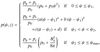
where the constants a, b, c, and d are chosen such that the pressure and its first derivative with respect to $\psi$ is a continuous function of $\psi$ and where we choose n=8. The three cases in Eq. (2) refer to the interior of the flux sheet, its boundary layer, and the ambient medium from top to bottom, respectively. The quantities $p_{\rm p}$ , $p_{\rm c}$ and p₀ are defined as,

$\displaystyle p_{\rm p} = p_{0,\rm p} {\rm e}^{-z/H_{\rm p}},$		(3)
$\displaystyle p_{\rm c} = p_{0,\rm c} {\rm e}^{-z/H_{\rm c}},$		(4)
$\displaystyle p_{0} = p_{0,\rm p} + p_{0,\rm c},$		(5)

where $H_{\rm p}$ and $H_{\rm c}$ are the photospheric and chromospheric pressure scale heights, respectively. We choose $H_{\rm p} = 110$ km and $H_{\rm c} = 220$ km. B₀ is the magnetic field strength on the axis of the flux sheet at the reference height z=0. The equation of motion along each field line reduces to the hydrostatic equation

$\begin{displaymath}\vec{B} \cdot [\nabla p - \rho \vec{g}] = 0, \end{displaymath}$

(6)

which defines us the density distribution and with it the temperature field. From the equation of motion perpendicular to $\vec{B}$ we obtain the electric current density

$\begin{displaymath}\vec{J} = \frac{1}{B^2} \vec{B} \times [\nabla p - \rho \vec{g}], \end{displaymath}$

(7)

which after some manipulation reduces to

$\begin{displaymath}\displaystyle j_{y} = \left. \frac{\partial p}{\partial \Psi}\right\vert _z\cdot \end{displaymath}$

(8)

The new magnetic field configuration can be calculated from the current density using the Grad-Shafranov equation,

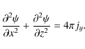
$\begin{displaymath}\frac{\partial^{2} \psi}{\partial x^{2}} + \frac{\partial^{2} \psi}{\partial z^{2}} = 4 \pi j_{y}. \end{displaymath}$

(9)

The above elliptic partial differential equation can be solved using standard numerical methods with appropriate boundary conditions. In practice we solve Eq. (9) on a computational domain that consists of only half of the flux sheet of horizontal and vertical extensions of 640 km and 1600 km, respectively. This domain is discretized on a equidistant rectangular mesh with a spacing of 5 km. The left side of the domain corresponds to the axis of the flux sheet. 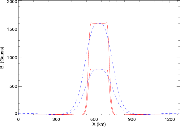The value of $\psi$ is prescribed at the left and the right side boundaries. At the top and bottom boundaries we use the Neumann condition $\partial\psi/\partial z = 0$ , assuming that the horizontal field component vanishes at these two boundaries. We treat two different cases corresponding to field strengths (at z = 0) of 800 G and 1600 G, on the axis of the sheet. For each of these cases we consider two boundary widths: 20 km and 80 km at the reference height z=0. These widths can be obtained by choosing appropriate values of $\psi_1$ and $\psi_2$ in Eq. (2).

$\begin{figure} \par\resizebox{8.8cm}{!}{\includegraphics{Version-Online/12450001.eps}} \end{figure}$	Figure 1: Vertical component of the magnetic field at the base of the flux sheet, z=0. Solid and dashed curves correspond to field configurations with a sharp and a wide interface to the weak-field surroundings, respectively. Each configuration is subdivided into a case of moderate field-strength with $\max(B_z)=800$ G and a case of strong field with $\max(B_z)=1600$ G.
Open with DEXTER

The vertical component of the magnetic field at z=0 is shown in Fig. 1 for the strong and moderate field cases. For the sharp interface (solid curves) the vertical component of the magnetic field component drops sharply, whereas in the case of a wide interface (dashed curves) the field decreases smoothly.

The characteristic properties of the two models are summarized in Table 1. The numbers in the first row of each quantity corresponds to the top boundary (z = 1600 km) and the numbers in the second row corresponds to the bottom boundary (z = 0 km). The temperature increases monotonically from 4758 K in the photosphere to 9142 K in the chromosphere corresponding to the sound speed variation from 7.1 km s^-1 to 13.5 km s^-1. The density and pressure at the axis of the sheet is the same for both the cases. We should mention that the ambient magnetic field is weak (of the order of few tens of Gauss). As we go higher up in the atmosphere the flux sheet expands and becomes uniform near the top with an average field strength of 118 G and 227 G for the moderate and strong field cases, respectively. The plasma- $\beta$ on the sheet axis is 1.69 and 0.42 at the base for the moderate and strong field cases.

3 Method and boundary conditions

Waves are excited in the equilibrium magnetic field configuration through a transverse motion of the lower boundary (similar to Hasan et al. 2005). The system of MHD equations, given in conservation-law form for an inviscid adiabatic fluid, is solved according to the method described in Steiner et al. (1994). These are the continuity, momentum, entropy, and the magnetic induction equations. The unknown variables are the density, $\rho$ , the momenta, $\rho V_{x}$ and $\rho V_{z}$ , where V_x and V_z are the horizontal and vertical components of the velocity, the entropy per unit mass, s, and the magnetic field, B_x and B_z. The equation of state is that for the solar mixture with a constant mean molecular weight of 1.297. For the numerical integration, the system of MHD equations are transformed into a system of discrete finite volume equations. The numerical fluxes are computed based on the flux-corrected transport (FCT) scheme of Oran & Boris (1987). For the induction equation we use a constrained transport scheme (Devore 1991), which automatically keeps $\nabla \cdot \vec{B} = 0$ . The time integration is explicit. The scheme is of second order accuracy.

Transmitting conditions apply to the side boundaries set by constant extrapolation of the variables from the physical domain to the boundary cells. Constant extrapolation also applies to the horizontal component of the momentum at the top and bottom boundary and to the vertical component at the bottom boundary. The density in the top boundary cells is determined using linear log extrapolation, while at the bottom boundary hydrostatic extrapolation applies. For the temperature constant extrapolation is used. The horizontal component of the magnetic field at the top and bottom boundaries are set equal to the corresponding values at the preceding interior point. The vertical component of the magnetic field is determined by the condition $\nabla \cdot \vec{B} = 0$ .

The transverse velocity V_x at z = 0 is specified as follows:

$\displaystyle V_{x}(x,0,t) = \left\{ \begin{array}{l l} \displaystyle V_{0} \si... ...~, \\ [1ex] \displaystyle 0 &\mbox{for}\quad 0 > t > P/2 , \end{array} \right.$

(10)

where V₀ denotes the amplitude of the horizontal motion and P is the wave period. This form was chosen to simulate the effect of transverse motion of the flux sheet at the lower boundary. For simplicity we assume that all points of the lower boundary have this motion: this does not generate any waves in the ambient medium, other than at the interface with the flux sheet. As a standard case in our simulation we use V₀ = 750 m s^-1 and P = 24 s following Hasan et al. (2005). This short period is motivated by the result of (Hasan et al. 2000) that high frequency waves would model the observational signature of wave heating less intermittent and thus in better agreement with the steady observed intensity from the magnetic network. We consider a uniform horizontal displacement of the bottom boundary for half a period after which the motion is stopped (this corresponds to the impulsive case treated by Hasan et al. 2005). Such short duration motions are expected to be generated by the turbulent motion in the convectively unstable subsurface layers where the flux sheet is rooted. In terms of the analysis by Cranmer & van Ballegooijen (2005) of the kinematics of G-band bright points, this motion rather corresponds to a short, single step of their ``random walk phase'', for which these authors use a rms velocity of 0.89 km s^-1 with a correlation time of bright-point motions of 60 s in accordance with the measurements of Nisenson et al. (2003). The cases with higher velocities (see Table 2) would rather be representative of the ``jump phase'' for which Cranmer & van Ballegooijen (2005) use a velocity of 5 km s^-1 with a duration of 20 s. This motion generates magnetoacoustic waves in the flux sheet. We first examine wave propagation and energy transport in a flux sheet with a sharp interface for the moderate and the strong field cases. In Sect. 6 we analyze the effect of varying the interface thickness.

$\begin{figure} \par\includegraphics[scale=.43,clip]{Version-Online/1245002d.eps}... ... \includegraphics[scale=.43,clip]{Version-Online/1245002a.eps}\\ \end{figure}$

Figure 2:

Temperature perturbations for the case in which the field strength at the axis at z=0 is 800 G (moderate field). The colors (gray shades for the print version) show the temperature perturbations at 40, 60, 80, and 120 s ( from bottom to top) after initiation of an impulsive horizontal motion at the z=0 boundary of a duration of 12 s with an amplitude of 750 m s^-1 and a period of P=24 s. The thin black curves are field lines and the white curve represents the contour of $\beta =1$ .

Open with DEXTER

4 Dynamics

4.1 Moderate field

$\begin{figure} { \begin{tabular}{cc} \includegraphics[scale=.35,clip]{Version-... ...ps}\\ \mbox{a) $V_{s}$ } & \mbox{b) $V_{n}$ } \end{tabular}} \end{figure}$

Figure 3:

Velocity components for the case in which the field strength at the axis at z=0 is 800 G (moderate field). The colors (gray shades for the print version) show the velocity components a) V_s, along the field, and b) V_n, normal to the field, at 40, 60, and 80 s ( from bottom to top) after initiation of an impulsive horizontal motion at the z=0 boundary of a duration of 12 s with an amplitude of 750 m s^-1 and a period of P=24 s. The thin black curves are field lines and the white curve represents the contour of $\beta =1$ . The field aligned and normal components of velocity are not shown in the regions where B < 50 G.

Open with DEXTER

Let us consider a magnetic configuration in which the field strength at the axis of the flux sheet at z=0 is 800 G. In this case the $\beta =1$ contour is well above the bottom boundary in the atmosphere and hence all the magnetic field lines emerging from the base of the sheet cross this layer at some height. Waves are excited at z=0, where $\beta >1$ (on the axis $\beta = 1.8$ ), in the form of a fast (predominantly acoustic) wave and a slow (predominantly magnetic) wave, which propagate respectively at the sound and the Alfvén speeds. On the sheet axis, the acoustic and Alfvén speeds at z=0 are 7.1 and 6.0 km s^-1, respectively (see Table 1). The fast wave is created due to compression and rarefaction of the gas at the leading and trailing edge of the flux sheet, respectively: this can be clearly discerned in the snapshots of the temperature perturbation, $\Delta T$ (the temperature difference with respect to the initial value), shown in Fig. 2 at 40, 60, 80 and 120 s after start of the perturbation. (These panels and panels in the following figures do not show the full height range of the computational domain but up to 1280 km only.) The black curves denote the magnetic field lines and the white curve depicts the $\beta =1$ contour. The perturbations are $180^\circ$ out of phase on opposite sides of the sheet axis. As these fast waves travel upwards they eventually cross the layer of $\beta =1$ , where they change their label from ``fast'' to ``slow'', without changing their acoustic nature: this corresponds to a ``mode transmission'' in the sense of Cally (2007). The transmission coefficient depends (among others) on the ``attack angle'' i.e., the angle between the wave vector and the local direction of the magnetic field (Cally 2007). On the $\beta =1$ layer, away from the sheet axis, where the wave vector is not exactly parallel to the magnetic field, we do not have complete transmission of the fast wave to a slow wave. Rather, there is a partial conversion of the mode from fast acoustic to fast magnetic, so that the energy in the acoustic mode is reduced correspondingly.

Figures 3a and 3b shows the velocity components in the flow parallel (V_s) and perpendicular (V_n) to the field, respectively. The velocity components are shown only in regions where the field is greater than 50 G since in the ambient medium with weak field this decomposition is no longer meaningful. In general the waves possess both longitudinal and transverse velocity components, but in regions where $\beta < 1$ , the parallel component essentially corresponds to the slow (acoustic) wave that is guided upward along the field. This correspondence can be seen by comparing the parallel flow pattern (in Fig. 3a) with the temperature perturbation in Fig. 2.

The excitation at the bottom boundary also generates a slow (magnetic) wave with velocity perturbations normal to the magnetic field line. In order to visualize the slow wave, we show the velocity component normal to the magnetic field in Fig. 3b. The slow wave also encounters the layer of $\beta =1$ and undergoes mode transmission and conversion. Above the layer of $\beta =1$ , the transmitted wave is a fast mode, which rapidly accelerates due to the sharp increase in Alfvén speed with height.

4.2 Strong field

We now consider the case in which the field strength on the sheet axis is 1600 G (at z=0). Here, the contour of $\beta =1$ approximately traces the boundary of the flux sheet. The transverse motion of the lower boundary generates slow (essentially acoustic) and fast (essentially magnetic) waves. Since the contour of $\beta =1$ runs along the boundary of the flux sheet, waves generated in the sheet that travel upwards do not encounter this layer and hence do not undergo mode conversion. Figure 4 shows the temperature perturbation $\Delta T$ at 40, 60, 80, and 120 s. Figure 5 shows the parallel and perpendicular components (with respect to the magnetic field) of the velocity.

The slow (acoustic) wave is guided upwards along the field without changing character. On the other hand, the fast wave, which can travel across the field encounters the $\beta =1$ contour at the boundary of the flux sheet. As the fast wave crosses this layer, it enters a region of negligible field and hence gets converted into a fast (acoustic) wave. This can be easily seen in the snapshot of temperature perturbations at an elapsed time of 40 s. The fast wave in the low- $\beta$ region, which is essentially a magnetic wave, undergoes mode conversion and becomes an acoustic wave, which creates fluctuations in temperature visible as wing like features in the periphery of the flux sheet between approximately z=200 to 500 km. The fast wave gets refracted due to the gradients in Alfvén speed higher up in the atmosphere. Furthermore, similar to Hasan et al. (2005), we find that the interface between the magnetic flux sheet and the ambient medium is a remarkable source of acoustic emission. It is visible in Fig. 4 as a wave of shell-like shape in the ambient medium that emanates from the base of the flux sheet and subsequently propagates, as a fast acoustic wave, laterally away from it.

Incidentally, the phase of transverse movement changes by $180^\circ$ between the moderate and strong field case as can be seen comparing Fig. 3b with Fig. 5b. This is due to the development of a vortical flow from the high pressure leading edge of the flux sheet to the low pressure trailing edge that develops in the high- $\beta$ photospheric layers of the moderately strong flux sheet but is largely suppressed in the strong field case, where it is from the beginning preceded by the fast (magnetic) wave that emerges right from the initial pulse. The development of a vortical flow in the moderate field case was also noticed in Hasan et al. (2005).

$\begin{figure} \par\includegraphics[scale=.39,clip]{Version-Online/1245004d.eps}... ... \includegraphics[scale=.39,clip]{Version-Online/1245004a.eps}\\ \end{figure}$	Figure 4: Temperature perturbations for the case in which the field strength at the axis at z=0 is 1600 G (strong field) for times t= 40, 60, 80, and 120 s. The coding corresponds to that of Fig. 2.
Open with DEXTER

$\begin{figure} \par { \begin{tabular}{cc} \includegraphics[scale=.35,clip]{Vers... ....eps}\\ \mbox{a) $V_{s}$ } & \mbox{b) $V_{n}$ } \end{tabular}} \end{figure}$	Figure 5: Velocity components for the case in which the field strength at the axis at z=0 is 1600 G (strong field) for times t= 40, 60, and 80 s. The coding corresponds to that of Fig. 3.
Open with DEXTER

Besides the fast and slow acoustic and the fast magnetic wave that emanate directly from the initial perturbation there is also a slow magnetic mode from this source, which propagates in the high- $\beta$ surface layer of the flux sheet. It is visible in Fig. 5b as the yellow/red crescent-shaped perturbation (bright shades for the print version), which trails the big red and blue crescents (white and black for the print version) pertaining to the fast magnetic mode. Different from the latter, which is maximal at the flux-sheet axis, the slow mode has maximal amplitude in the weak-field boundary-layer of the flux concentration. A similar but acoustic slow surface mode was found by Khomenko et al. (2008) when the driver was located in the high- $\beta$ layers of the flux concentration. Here, this mode generates a remarkable amount of acoustic emission to the ambient medium as will be seen in Sect. 6.

In a three-dimensional environment there would in general appear a third, intermediate wave type, additional to the slow and fast mode, depending on the geometry of the magnetic field and the initial perturbation. Correspondingly, we may expect mode coupling between all three wave types. In the presence of gravitational stratification, the $\beta =1$ surface (more precisely the surface of equal Alfvén and sound speed) would still constitute the critical layer for mode coupling so that we could expect scenarios not radically different from but more complex than those of Sects. 4.1 and 4.2.

$\begin{figure} \begin{tabular}{cc} \includegraphics[scale=.35,clip]{Version-Onl... ...1.eps} \\ \mbox{a) Acoustic} & \mbox{b) Poynting} \end{tabular} \end{figure}$

Figure 6:

Wave-energy fluxes (absolute values) for the case in which the field strength at the axis at z=0 is 800 G (moderate field). The colors (gray shades for the print version) show a) the acoustic flux, and b) the Poynting flux, at 40, 60, and 80 s ( from bottom to top) after initiation of an impulsive horizontal motion at the z=0 boundary of a duration of 12 s with an amplitude of 750 m s^-1 and a period of P=24 s. The thin black curves are field lines and the thick black curve represents the contour of $\beta =1$ . The Poynting fluxes are not shown in the ambient medium where B < 50 G.

Open with DEXTER

5 Energy transport

We now consider the transport of energy in the various wave modes. Using the full nonlinear expression for the energy flux, it is not easily possible to identify the amount of energy carried by the magnetic and acoustic waves. Following Bogdan et al. (2003), we instead consider the wave flux using the expression given by Bray & Loughhead (1974) that represents the net transport of energy into the atmosphere:

$\begin{displaymath}\vec{F}_{\rm wave} = \Delta p\vec{V} + \frac{1}{4 \pi}(\vec{B... ...} - \frac{1}{4 \pi}(\vec{V} \cdot \Delta \vec{B})\vec{B}_{0} . \end{displaymath}$

(11)

The first term on the right hand side of the equality sign is the net acoustic flux, and the last two terms are the net Poynting flux. The operator $\Delta$ gives the perturbations in the variable with respect to the initial equilibrium solution and B₀ refers to the unperturbed magnetic field.

Figures 6a and 6b show the magnitude of the acoustic (left panels) and the Poynting flux (right panels) at 40, 60, and 80 s (from bottom to top) for the moderate field case. Since in the ambient medium the field strength is weak, the Poynting fluxes are not shown in this region. The Poynting flux is essentially the wave energy that is carried by the magnetic mode, which as expected, is localized to the flux sheet. On the other hand, the energy transport in the acoustic-like component is more isotropic. At t=40 s, we find from Fig. 6a that the wave has just crossed the $\beta =1$ contour. Thereafter, it propagates as a slow wave guided along the field at the acoustic speed within the flux sheet and as a fast spherical-like wave in the surrounding quasi field-free medium. Inside the flux sheet, the energy in the magnetic component (Poynting flux) and the acoustic component is of the same order of magnitude.

A comparison of these results with those for the strong field case (Fig. 7) shows that in the latter case energy is transported by the fast wave much more rapidly, especially in the central regions of the flux sheet. This is due to the sharp increase of the Alfvén speed with height above z > 200 km. At t=40 s we find that the wave front associated with the magnetic component has already reached a height of about 500 km (close to the sheet axis), while the acoustic wave reaches this level only at about t=80 s.

From the contour plots of Figs. 6 and 7, we see that the fluxes in the ambient medium for the strong field case is still close to 10⁸ erg cm^-2 s^-1, while for the moderate field, it is almost an order of magnitude less, suggesting that the flux sheets with strong fields are a more efficient source of acoustic fluxes into the ambient medium. The ``mode transmission'' from fast (acoustic) to slow (acoustic) that takes place in the case of a moderate field, as explained in Sect. 4, can be seen in Fig. 6a. Since the ``attack angle'' in this case is close to zero, a significant amount of acoustic transmission takes place across the layer of $\beta =1$ . Another feature that we see in the plots of wave-energy fluxes is the ``mode conversion'' that takes place in the strong field case. The fast magnetic wave, which is generated inside the flux sheet can travel across the magnetic field. This mushroom like shape, which is expanding, can be easily discerned in the 40 s snapshot of the Poynting flux shown in Fig. 7b. As this wave crosses the $\beta =1$ contour, it is converted into a fast (acoustic) wave. The wing like feature that can be seen in the 60 s snapshot of the acoustic fluxes (Fig. 7a) are due to the fast waves that have a moment ago undergone a ``mode conversion'' from magnetic to acoustic.

Next we consider a field line to the left of the flux sheet axis, which encloses a fractional flux of 50%. The field aligned and the normal component of the wave-energy fluxes are calculated along this particular field line. Figure 8 shows the positive, field aligned component of acoustic flux for the moderate and strong field case as a function of time and spatial coordinate z along the field line. The dotted curves in the figure show the space time position of a hypothetical wavefront that travels with Alfvén speed (steeper slope) and sound speed along this magnetic field line. With the help of this plots it is easy to separate the energy fluxes that is carried by the slow and the fast wave modes. The evolution of the $\beta =1$ layer is shown for the moderate field case. The perturbation of this layer as the wave crosses it can be seen clearly around 40 s. It moves down due to the decrease in pressure caused by the rarefaction front and then moves up when the compression front passes it. Most fraction of the flux lies parallel to the line that corresponds to the hypothetical acoustic wave, which is a slow mode in the region where $\beta < 1$ . In the strong field case, above approximately z=800 km and for times $t \ga 120$ s, the acoustic flux carried in the compressive (trailing) phase starts to catch up the slightly slower moving expansive phase and the flux gets confined into a narrow shock forming region. This is also visible in the case of the moderately strong field. This behavior is not present along the corresponding field line to the right of the sheet axis (not shown here), where the compressive phase is leading so that the compressive and expansive phase of the perturbation slightly diverge with time.

$\begin{figure} \begin{tabular}{cc} \includegraphics[scale=.35,clip]{Version-Onl... ...1.eps}\\ \mbox{a) Acoustic} & \mbox{b) Poynting} \end{tabular} \end{figure}$	Figure 7: Wave-energy fluxes for the case in which the field strength at the axis at z=0 is 1600 G (strong field) for times t= 40, 60, and 80 s. The coding corresponds to that of Fig. 6. The Poynting fluxes are not shown in the ambient medium where B < 200 G.
Open with DEXTER

$\begin{figure} \par\mbox{\includegraphics[scale=.4,clip]{Version-Online/1245008a.eps} \includegraphics[scale=.4,clip]{Version-Online/1245008b.eps} } \end{figure}$	Figure 8: The field aligned positive (upwardly directed) component of acoustic wave-energy flux as a function of time on a field line on the left side of the axis that encloses a fractional flux of 50%. The left panel represents the case in which the field strength at the axis at z=0 is 800 G (moderate field) and the right panel represents the strong field case (1600 G).
Open with DEXTER

$\begin{figure} \par\mbox{\includegraphics[scale=.4,clip]{Version-Online/1245009a.eps} \includegraphics[scale=.4,clip]{Version-Online/1245009b.eps} } \end{figure}$	Figure 9: The field aligned positive (upwardly directed) component of the Poynting flux as a function of time on a field line on the left side of the axis that encloses a fractional flux of 50%. The left panel represents the case in which the field strength at the axis at z=0 is 800 G (moderate field) and the right panel represents the strong field case (1600 G).
Open with DEXTER

Table 2: Temporal maximum of the horizontally averaged, vertical component of the wave-energy fluxes for the strong field case.

The acoustic fluxes are of the order 10⁷ erg cm^-2 s^-1. The Poynting fluxes carried by the fast mode in this region can be identified by the coloured contours (grays shades for the print version) that gather along the dotted curves corresponding to the hypothetical Alfvén wave (Fig. 9). Comparing the two fluxes (Fig. 9 with Fig. 8), it is clear that the acoustic flux carried by the slow mode is larger than the Poynting flux, especially in the moderate field case. The Poynting flux rapidly weakens with time and height because it is not guided along the field lines like the slow mode but rapidly diverges across the field and part of the Poynting flux converts to acoustic again as explained in Sect. 4. Also from Fig. 9 it can be seen that while the magnetically dominated fast mode starts right from the excitation level at z=0 in the strong field case, it starts in the weak field case only after about 40 s when the fast acoustic wave reaches the conversion layer where $\beta \approx 1$ and partially undergoes mode conversion. Therefore, the fast (magnetic) mode is from the beginning weaker in the moderate as compared to the strong field case.

Table 2 shows the temporal maximum of the horizontally averaged vertical components of acoustic and Poynting fluxes at three different heights for the strong field case. We have considered three different amplitudes and periods for the initial excitations. Although the field aligned acoustic fluxes on the specific field line considered in Fig. 8 reach values of the order of 10⁷ erg cm^-2 s^-1 at a height of z=1000 km, the horizontally averaged fluxes are typically an order of magnitude less, depending upon the amplitude of the initial excitation. The Poynting fluxes shown in the table are the maximum value that the fluxes reach in the interval between the start of the simulation until the time when the fast wave reaches the top boundary (around 60 s). Hence these fluxes are due to the fast mode for z=500 km and z=1000 km, since within this time limit the slow mode has not yet reached these heights. The Poynting fluxes associated with the fast mode are relatively lower in magnitude compared to the acoustic fluxes. It should be noted that there is also considerable Poynting flux associated with the slow mode, since these waves also perturb the magnetic field. The acoustic fluxes of the moderate field case reach only less than 70% of that of the strong field configuration and the Poynting fluxes are negligible in this case.

6 Effects of the boundary-layer width

We now study the acoustic emission of the magnetic flux concentrations into the ambient medium by varying the width of the boundary layer between the flux sheet and ambient medium. This is carried out by comparing the result of simulations with a sharp interface of width 20 km to that with a width of 80 km (see Fig. 1), where the width can be varied by choosing appropriate values of $\psi_1$ and $\psi_2$ in Eq. (2).

We examine the acoustic emission from the two peripheral (control) field lines to the left and to the right of the flux-sheet axis that encompass 90% of the magnetic flux. These correspond to the outermost field lines that are plotted in Figs. 2 to 7. These field lines are located in the high- $\beta$ region with $\beta \gg 1$ , all the way from the base to the merging height, where the flux sheet starts to fill the entire width of the computational domain. The acoustic emission from the peripheral field line to the right and to the left of the flux-sheet axis is practically identical.

Figure 10 shows the acoustic emission from the flux sheet into the ambient medium for the peripheral field line to the left of the flux sheet with the strong field (B₀=1600 G) and the cases of the sharp interface (left panel) and the wide interface (right panel). Concentrating on the case with the sharp interface first, we see that acoustic flux is initially generated by the fast mode that stems from the transversal motion of the flux sheet to the right hand side, which causes a compression and expansion to the right and left side of the flux-sheet edge, respectively. This movement generates a net acoustic flux away from the flux sheet on both sides. It is visible in Figs. 4 and 7 as the shell-like antisymmetric wave that emanates from the base of the flux sheet propagating into the ambient medium. At a height of z=100 km the peak value of this flux is $3\times 10^8$ erg cm^-2 s^-1 for the sharp interface but only $1.2\times 10^8$ erg cm^-2 s^-1 for the wide interface. This is because the sharp interface acts like a hard wall that pushes against the ambient medium, while the wide interface is more compressible and acts more softly.

$\begin{figure} \par\mbox{\subfigure{\includegraphics[scale=0.4,clip]{1245010a.eps} } \subfigure{\includegraphics[scale=0.4,clip]{1245010b.eps} }} \end{figure}$	Figure 10: Acoustic flux perpendicular to the peripheral field lines that encompass 90% of the magnetic flux as a function of time and height along the field line. Only the outwardly directed flux is shown. Left: strong field case with a sharp interface between flux-sheet interior and ambient medium. Right: strong field case with a wide interface.
Open with DEXTER

Near the flux-sheet boundary this wave seamlessly connects to the tips of the crescent-like fast (magnetic) mode of the flux-sheet interior as can be best seen when comparing the first two snapshots of Figs. 4 and 5b. There, acoustic flux is generated by continuous leakage and conversion from the magnetic mode, giving rise to the steeper of the two horizontally running, inclined ridges of acoustic flux, visible in the lower part of both panels of Fig. 10. This leakage is more efficient in the case of the wide interface than in the case to the sharp interface so that the corresponding ridge extends over a longer period of time in the former compared to the latter case. However, it cannot compensate for the larger initial flux that emanates from the more confined (sharp) boundary.

Starting at about t=25 s in case of the sharp interface, one can see a less steep and weaker branch of acoustic flux that is connected to the slow (magnetic) mode that propagates in the high- $\beta$ boundary-layer of the flux sheet. Obviously it creates a non-negligible source of acoustic flux to the ambient medium. It is also present in case of the wide interface.

The two horizontally running ridges of acoustic flux in the case of the sharp interface (Fig. 10, left) is slightly more inclined compared to the case with the wide interface (Fig. 10, left), where the peripheral (control) field line expands more in the horizontal direction so that the wave travels a longer distance to reach it.

At approximately t=45 s we start to see acoustic flux appearing at a height of about z=1000 km. This flux originates from the refracted fast (magnetic) wave within the flux sheet. Since this wave quickly accelerates and refracts with height, it reaches the flux-sheet boundary sooner at z=1000 km than in the height range 500 km < z < 800 km. This wave undergoes conversion from fast, predominantly magnetic to fast, predominantly acoustic as it crosses the region where $\beta =1$ . Because it travels essentially perpendicular to the field near the flux-sheet boundary, the conversion is particularly efficient. While this ridge of acoustic flux originates from the leading phase of the fast (magnetic) wave that corresponds to a movement to the right (red [white] big crescent in the 40 s snapshot of Fig. 5b), a second, parallel running negative ridge, stems from the following phase, corresponding to a movement to the left (blue [black] crescent in the 40 s snapshot of Fig. 5b).

Table 3 shows the total acoustic emission to the ambient medium, still from and perpendicularly across the field lines that encompasses 90% of the total magnetic flux for cases with 3 different boundary layer widths. The energy is computed by integration of the perpendicular flux along the peripheral control field lines to the left and to the right over the full height range of the computational domain and from t=0 s to t=64 s for unit width. The total acoustic energy leaving the flux sheet with the wide interface is only 35% of that with the sharp interface. In this sense, a flux sheet with a sharp interface is more efficient in providing acoustic flux to the ambient medium than a flux sheet with a wide interface as conjectured by Hasan et al. (2005).

Table 3: Total acoustic emission from the flux sheet into the ambient medium for different boundary layer widths.

7 Summary

This work is an extension of the previous work done by Hasan et al. (2005). Wave excitation occurs in a magnetic flux concentration by a transverse motion of the base. The present work extends the previous calculations to the case of a flux sheet with moderate field strength. In addition, a new feature of the present work is that we estimate the energy carried by the waves and we examine the effect of varying the thickness of the tube-ambient medium interface on the acoustic emission.

We have found that the nature of the modes excited depends upon the value of $\beta$ in the region where the driving motion occurs. When $\beta$ is large, the slow wave is a transverse magnetic mode that propagates along the field lines and undergoes mode transmission as it crosses the $\beta =1$ layer. In this case, the wave only changes label from slow to fast, but remains magnetic in character throughout the flux sheet. The fast mode, which propagates almost isotropically, undergoes both mode conversion and transmission at the $\beta =1$ surface depending on the ``attack angle'', the angle between the wave vector and the magnetic field. On the other hand, in the case of a strong magnetic field (low- $\beta$ case), where the level of $\beta =1$ is below the driving region, the fast (magnetic) and slow (acoustic) modes propagate through the flux sheet atmosphere without changing character.

We find that the magnetically dominated fast wave within the low- $\beta$ region of the flux sheet undergoes strong refraction so that it finally leaves the flux sheet in the lateral direction, where it gets partially and mainly converted to a fast, acoustically dominated wave. This effect is particularly visible in the case of a flux sheet with strong magnetic field.

We also see an asymmetry in the wave structure on both sides of the flux sheet axis. This comes because the leading front of the predominantly acoustic mode is compressional on the one hand side and expansive on the other side and vice versa for the following phase. Since the compressive phase travels faster as the sound speed is larger, the two phases move either apart from each other or converge. In principle, this asymmetry should give rise to observable signatures.

Recent observations of the chromospheric network are suggestive of Ca II network grains associated with plasma with quasi-steady heating at heights between 0.5 and 1 Mm inside magnetic flux concentrations (Hasan & van Ballegooijen 2008). Let us now estimate the acoustic energy flux transported into the chromosphere through a single short duration pulse as has been treated in the present paper (the magnetic modes are almost incompressible and not efficient for heating the atmosphere). We consider the energy flux at a height of 1000 km. For the strong and moderate field cases, the maximum values of the acoustic fluxes at z=1000 km are $\sim$ $15\times 10^{6}$ erg cm^-2 s^-1 and $\sim$ $5\times 10^{6}$ erg cm^-2 s^-1, respectively. However, it should be noted that although the fluxes can reach values up to 10⁷ erg cm^-2 s^-1, the spatially averaged values are much less. From Table 2 we obtain for the strong field case a temporal maximum of the horizontally averaged acoustic flux at z=1000 km of a few times 10⁶ erg cm^-2 s^-1, depending on the excitation amplitude and period.

We see that the strong field configuration is a more efficient source of acoustic waves in the ambient medium compared to the weak to moderate field configurations. For the cases considered here, they differ by almost a factor of two. The width of the transition layer between the flux sheet and the ambient medium has significant effect on the acoustic wave emission as was initially conjectured by Hasan et al. (2005). Our quantitative calculations substantiate this hypothesis: a flux sheet with a sharp interface emits almost four times the energy emitted by a flux sheet with a wide interface.

8 Discussion and conclusion

The energy losses in the magnetic network at chromospheric heights are of the order of 10⁷ erg cm^-2 s^-1. Even though the acoustic energy flux produced by the transverse excitation movement can temporarily reach this value at certain locations, the values of Table 2 tell us that in the spatial average these energy losses cannot be balanced by the acoustic energy flux generated in our model. This conclusion is emphasized by the fact that the values of Table 2 are temporal maxima: the temporal mean would be lower. In order to be compatible with the observed quasi-steady Ca emission the injection of energy needs to be in the form of sustained short duration pulses as argued by (Hasan & van Ballegooijen 2008) but these pulses could probably not maintain the maximum values of acoustic flux as quoted in Table 2.

Possibly with the exception of the case corresponding to the last row in Table 2, the transverse excitation considered here rather correspond to the ``random walk phase'' of the model by Cranmer & van Ballegooijen (2005). Excitations corresponding to the ``jump phase'' with even higher velocity amplitudes than considered in the present paper might temporarily be capable of providing the required energy flux. However, with a mean interval time of 360 s these jump events are probably not responsible for the heating observed in Ca II network grains, which requires a more steady or high frequency source.

We have not considered photospheric radiative losses, which would considerably damp the waves before they reach chromospheric heights (Carlsson & Stein 2002). If these radiative losses are taken into account, the fluxes would further be lowered. Also not all of the acoustic energy flux would be available for radiative energy loss in the chromosphere depending on the details of this NLTE process. All this implies that acoustic waves generated by transverse motions of the footpoints of magnetic network elements cannot balance the chromospheric energy requirements of network regions.

This conclusion cannot be expected to drastically change when turning to three spatial dimensions. The details of the mode coupling and the partition of energy fluxes to the various modes would become more complex but the share of energy that resides in the acoustic mode cannot be much larger than in the two-dimensional case. On the contrary, the energy flux generated at the footpoint of the magnetic element would have to be distributed to a larger area in three spatial dimension so that the spatial mean at z=1000 km would be lower.

We have only considered single, short duration, transverse pulses for the wave excitation. A more realistic driver with sustained pulses of varying lengths, velocities, and time intervals would give rise to highly non-linear dynamics, which might yield increased acoustic fluxes. Also we have not considered longitudinal wave excitation, which would be available primarily from global p-mode oscillations. The latter are expected to provide low frequency slow mode waves to the outer atmosphere via magnetic portals in the presence of inclined strong magnetic fields, where they would be available for dissipation through shock formation (Jefferies et al. 2006; Suematsu 1990; Michalitsanos 1973; Hansteen et al. 2006). In fact, thismechanism would also work in the periphery of a vertically oriented flux tube, where the field is strongly inclined with respect to the vertical direction. Another source of energy that was not considered here may come from direct dissipation of magnetic fields through Ohmic dissipation.

Acknowledgements

We thank R. Schlichenmaier for valuable comments on the manuscript. The report by the anonymous referee, which helped greatly improve the presentation, are gratefully acknowledged. This work was supported by the German Academic Exchange Service (DAAD), grant D/05/57687, and the Indian Department of Science & Technology (DST), grant DST/INT/DAAD/P146/2006.

References

Berger, T. E., & Title, A. M. 1996, ApJ, 463, 365 [NASA ADS] [CrossRef]
Berger, T. E., & Title, A. M. 2001, ApJ, 553, 449 [NASA ADS] [CrossRef]
Berger, T. E., Rouppe van der Voort, L. H. M., Löfdahl, M. G., et al. 2004, A&A, 428, 613 [NASA ADS] [EDP Sciences] [CrossRef]
Bogdan, T. J., Carlsson, M., Hansteen, V. H., et al. 2003, ApJ, 599, 626 [NASA ADS] [CrossRef]
Bray, R. J., & Loughhead, R. E. 1974, The solar chromosphere, The International Astrophysics Series (London: Chapman and Hall)
Cally, P. S. 2005, MNRAS, 358, 353 [NASA ADS] [CrossRef]
Cally, P. S. 2007, Astron. Nachr., 328, 286 [NASA ADS] [CrossRef]
Carlsson, M., & Stein, R. F. 2002, in SOLMAG Proceedings of the Magnetic Coupling of the Solar Atmosphere Euroconference, ed. H. Sawaya-Lacoste, ESA SP-505, 293
Cranmer, S. R., & van Ballegooijen, A. A. 2005, ApJS, 156, 265 [NASA ADS] [CrossRef]
De Pontieu, B., Hansteen, V. H., Rouppe van der Voort, L., van Noort, M., & Carlsson, M. 2007, ApJ, 655, 624 [NASA ADS] [CrossRef]
Devore, C. R. 1991, J. Comp. Phys., 92, 142 [NASA ADS] [CrossRef]
Grossmann-Doerth, U., Kneer, F., & Uexküll, M. V. 1974, Sol. Phys., 37, 85 [NASA ADS] [CrossRef]
Hansteen, V. H., De Pontieu, B., Rouppe van der Voort, L., van Noort, M., & Carlsson, M. 2006, ApJ, 647, L73 [NASA ADS] [CrossRef]
Hasan, S. S., & Ulmschneider, P. 2004, A&A, 422, 1085 [NASA ADS] [EDP Sciences] [CrossRef]
Hasan, S. S., & van Ballegooijen, A. A. 2008, ApJ, 680, 1542 [NASA ADS] [CrossRef]
Hasan, S. S., Kalkofen, W., & van Ballegooijen, A. A. 2000, ApJ, 535, L67 [NASA ADS] [CrossRef]
Hasan, S. S., van Ballegooijen, A. A., Kalkofen, W., & Steiner, O. 2005, ApJ, 631, 1270 [NASA ADS] [CrossRef]
Jefferies, S. M., McIntosh, S. W., Armstrong, J. D., et al. 2006, ApJ, 648, L151 [NASA ADS] [CrossRef]
Khomenko, E., Collados, M., & Felipe, T. 2008, Sol. Phys., 251, 589 [NASA ADS] [CrossRef]
Lites, B. W., Rutten, R. J., & Kalkofen, W. 1993, ApJ, 414, 345 [NASA ADS] [CrossRef]
Michalitsanos, A. G. 1973, Sol. Phys., 30, 47 [NASA ADS] [CrossRef]
Muller, R. 1985, Sol. Phys., 100, 237 [NASA ADS] [CrossRef]
Muller, R., Roudier, T., Vigneau, J., & Auffret, H. 1994, A&A, 283, 232 [NASA ADS]
Nisenson, P., van Ballegooijen, A. A., de Wijn, A. G., & Sütterlin, P. 2003, ApJ, 587, 458 [NASA ADS] [CrossRef]
Oran, E. S., & Boris, J. P. 1987, Numerical Simulation of Reactive Flow (Elsevier)
Rosenthal, C. S., Bogdan, T. J., Carlsson, M., et al. 2002, ApJ, 564, 508 [NASA ADS] [CrossRef]
Schaffenberger, W., Wedemeyer-Böhm, S., Steiner, O., & Freytag, B. 2005, in Chromospheric and Coronal Magnetic Fields, ed. D. E. Innes, A. Lagg, & S. A. Solanki, ESA SP-596, 65
Sheminova, V. A., Rutten, R. J., & Rouppe van der Voort, L. H. M. 2005, A&A, 437, 1069 [NASA ADS] [EDP Sciences] [CrossRef]
Solanki, S. K. 1993, Space Sci. Rev., 63, 1 [NASA ADS] [CrossRef]
Steiner, O., Pneuman, G. W., & Stenflo, J. O. 1986, A&A, 170, 126 [NASA ADS]
Steiner, O., Knölker, M., & Schüssler, M. 1994, in Solar Surface Magnetism, ed. R. J. Rutten, & C. J. Schrijver, 441
Steiner, O., Vigeesh, G., Krieger, L., et al. 2007, Astron. Nachr., 328, 323 [NASA ADS] [CrossRef]
Suematsu, Y. 1990, in Progress of Seismology of the Sun and Stars, ed. Y. Osaki, & H. Shibahashi (Berlin: Springer Verlag), Lect. Notes Phys., 367, 211

Footnotes

... magnetic): For brevity we call modes in the following simply acoustic and magnetic depending on the predominance of the thermal and magnetic nature of their restoring forces.
... 120 s: The temperature perturbations along the flux-sheet edges in the wake of the slow acoustic wave (red and blue ridges [black and white for the print version] along the left and right boundary in the lower part of the flux sheet, respectively) do not pertain to a traveling wave. They are due to the finite shift of the flux sheet with respect to the initial, static configuration. This shift is compensated for by a corresponding shift of the unperturbed solution for the computation of energy fluxes in Sects. 5 and 6.

All Tables

Table 1: Equilibrium model parameters for the moderate and strong flux sheets.

Table 2: Temporal maximum of the horizontally averaged, vertical component of the wave-energy fluxes for the strong field case.

Table 3: Total acoustic emission from the flux sheet into the ambient medium for different boundary layer widths.

All Figures

$\begin{figure} \par\resizebox{8.8cm}{!}{\includegraphics{Version-Online/12450001.eps}} \end{figure}$	Figure 1: Vertical component of the magnetic field at the base of the flux sheet, z=0. Solid and dashed curves correspond to field configurations with a sharp and a wide interface to the weak-field surroundings, respectively. Each configuration is subdivided into a case of moderate field-strength with $\max(B_z)=800$ G and a case of strong field with $\max(B_z)=1600$ G.
Open with DEXTER
In the text

$\begin{figure} \par\includegraphics[scale=.43,clip]{Version-Online/1245002d.eps}... ... \includegraphics[scale=.43,clip]{Version-Online/1245002a.eps}\\ \end{figure}$	Figure 2: Temperature perturbations for the case in which the field strength at the axis at z=0 is 800 G (moderate field). The colors (gray shades for the print version) show the temperature perturbations at 40, 60, 80, and 120 s ( from bottom to top) after initiation of an impulsive horizontal motion at the z=0 boundary of a duration of 12 s with an amplitude of 750 m s^-1 and a period of P=24 s. The thin black curves are field lines and the white curve represents the contour of $\beta =1$ .
Open with DEXTER
In the text

$\begin{figure} { \begin{tabular}{cc} \includegraphics[scale=.35,clip]{Version-... ...ps}\\ \mbox{a) $V_{s}$ } & \mbox{b) $V_{n}$ } \end{tabular}} \end{figure}$	Figure 3: Velocity components for the case in which the field strength at the axis at z=0 is 800 G (moderate field). The colors (gray shades for the print version) show the velocity components a) V_s, along the field, and b) V_n, normal to the field, at 40, 60, and 80 s ( from bottom to top) after initiation of an impulsive horizontal motion at the z=0 boundary of a duration of 12 s with an amplitude of 750 m s^-1 and a period of P=24 s. The thin black curves are field lines and the white curve represents the contour of $\beta =1$ . The field aligned and normal components of velocity are not shown in the regions where B < 50 G.
Open with DEXTER
In the text

$\begin{figure} \par\includegraphics[scale=.39,clip]{Version-Online/1245004d.eps}... ... \includegraphics[scale=.39,clip]{Version-Online/1245004a.eps}\\ \end{figure}$	Figure 4: Temperature perturbations for the case in which the field strength at the axis at z=0 is 1600 G (strong field) for times t= 40, 60, 80, and 120 s. The coding corresponds to that of Fig. 2.
Open with DEXTER
In the text

$\begin{figure} \par { \begin{tabular}{cc} \includegraphics[scale=.35,clip]{Vers... ....eps}\\ \mbox{a) $V_{s}$ } & \mbox{b) $V_{n}$ } \end{tabular}} \end{figure}$	Figure 5: Velocity components for the case in which the field strength at the axis at z=0 is 1600 G (strong field) for times t= 40, 60, and 80 s. The coding corresponds to that of Fig. 3.
Open with DEXTER
In the text

$\begin{figure} \begin{tabular}{cc} \includegraphics[scale=.35,clip]{Version-Onl... ...1.eps} \\ \mbox{a) Acoustic} & \mbox{b) Poynting} \end{tabular} \end{figure}$	Figure 6: Wave-energy fluxes (absolute values) for the case in which the field strength at the axis at z=0 is 800 G (moderate field). The colors (gray shades for the print version) show a) the acoustic flux, and b) the Poynting flux, at 40, 60, and 80 s ( from bottom to top) after initiation of an impulsive horizontal motion at the z=0 boundary of a duration of 12 s with an amplitude of 750 m s^-1 and a period of P=24 s. The thin black curves are field lines and the thick black curve represents the contour of $\beta =1$ . The Poynting fluxes are not shown in the ambient medium where B < 50 G.
Open with DEXTER
In the text

$\begin{figure} \begin{tabular}{cc} \includegraphics[scale=.35,clip]{Version-Onl... ...1.eps}\\ \mbox{a) Acoustic} & \mbox{b) Poynting} \end{tabular} \end{figure}$	Figure 7: Wave-energy fluxes for the case in which the field strength at the axis at z=0 is 1600 G (strong field) for times t= 40, 60, and 80 s. The coding corresponds to that of Fig. 6. The Poynting fluxes are not shown in the ambient medium where B < 200 G.
Open with DEXTER
In the text

$\begin{figure} \par\mbox{\includegraphics[scale=.4,clip]{Version-Online/1245008a.eps} \includegraphics[scale=.4,clip]{Version-Online/1245008b.eps} } \end{figure}$	Figure 8: The field aligned positive (upwardly directed) component of acoustic wave-energy flux as a function of time on a field line on the left side of the axis that encloses a fractional flux of 50%. The left panel represents the case in which the field strength at the axis at z=0 is 800 G (moderate field) and the right panel represents the strong field case (1600 G).
Open with DEXTER
In the text

$\begin{figure} \par\mbox{\includegraphics[scale=.4,clip]{Version-Online/1245009a.eps} \includegraphics[scale=.4,clip]{Version-Online/1245009b.eps} } \end{figure}$	Figure 9: The field aligned positive (upwardly directed) component of the Poynting flux as a function of time on a field line on the left side of the axis that encloses a fractional flux of 50%. The left panel represents the case in which the field strength at the axis at z=0 is 800 G (moderate field) and the right panel represents the strong field case (1600 G).
Open with DEXTER
In the text

$\begin{figure} \par\mbox{\subfigure{\includegraphics[scale=0.4,clip]{1245010a.eps} } \subfigure{\includegraphics[scale=0.4,clip]{1245010b.eps} }} \end{figure}$	Figure 10: Acoustic flux perpendicular to the peripheral field lines that encompass 90% of the magnetic flux as a function of time and height along the field line. Only the outwardly directed flux is shown. Left: strong field case with a sharp interface between flux-sheet interior and ambient medium. Right: strong field case with a wide interface.
Open with DEXTER
In the text

Current usage metrics show cumulative count of Article Views (full-text article views including HTML views, PDF and ePub downloads, according to the available data) and Abstracts Views on Vision4Press platform.

Data correspond to usage on the plateform after 2015. The current usage metrics is available 48-96 hours after online publication and is updated daily on week days.

Initial download of the metrics may take a while.