| Issue |
A&A
Volume 508, Number 2, December III 2009
|
|
|---|---|---|
| Page(s) | 941 - 950 | |
| Section | The Sun | |
| DOI | https://doi.org/10.1051/0004-6361/200912275 | |
| Published online | 27 August 2009 | |
A&A 508, 941-950 (2009)
Acoustic waves in the solar atmosphere at high spatial resolution
N. Bello González1,2 - M. Flores Soriano2 - F. Kneer2 - O. Okunev2,3
1 - Kiepenheuer-Institut für Sonnenphysik, Schöneckstr. 6, 79104 Freiburg, Germany
2 -
Institut für Astrophysik, Friedrich-Hund-Platz 1, 37077 Göttingen, Germany
3 -
Central Astronomical Observatory of the Russian Academy of Sciences, Pulkovskoye chaussee 65/1, 196140 St. Petersburg, Russia
Received 4 April 2009 / Accepted 10 August 2009
Abstract
Aims. The energy supply for the radiative losses of the
quiet solar chromosphere is studied. On the basis of high spatial
resolution data, we investigate the amount of energy flux carried by
acoustic waves in the solar photosphere.
Methods. Time sequences from quiet Sun disc centre were obtained
with the ``Göttingen'' Fabry-Perot spectrometer at the Vacuum Tower
Telescope, Observatorio del Teide/Tenerife, in the non-magnetic Fe I 5576 Å
line. The data were reconstructed with speckle methods. The velocity
and intensity fluctuations at line minimum were subjected to Fourier
and wavelet analyses. The energy fluxes at frequencies higher than the
acoustic cutoff frequency (period
![]() s) were corrected for the transmission of the solar atmosphere, which reduces the signal from short-period waves.
s) were corrected for the transmission of the solar atmosphere, which reduces the signal from short-period waves.
Results. Both Fourier and wavelet analysis give an amount of energy flux of ![]() 3000 W m-2 at a height h=250 km.
Approximately 2/3 of it is carried by waves in the 5-10 mHz
range, and 1/3 in the 10-20 mHz band. Extrapolation of the
flux spectra gives an energy flux of 230-400 W m-2 at frequencies
3000 W m-2 at a height h=250 km.
Approximately 2/3 of it is carried by waves in the 5-10 mHz
range, and 1/3 in the 10-20 mHz band. Extrapolation of the
flux spectra gives an energy flux of 230-400 W m-2 at frequencies ![]() > 20 mHz. We find that the waves occur predominantly above inter-granular areas.
> 20 mHz. We find that the waves occur predominantly above inter-granular areas.
Conclusions. We conclude that the acoustic flux in waves with
periods shorter than the acoustic cutoff period can contribute to the
basal heating of the solar chromosphere, in addition to the atmospheric
gravity waves found recently.
Key words: Sun: photosphere - Sun: chromosphere - Sun: oscillations - techniques: high angular resolution - techniques: spectroscopic
1 Introduction
According to standard, hydrostatic models of the solar atmosphere (Maltby et al. 1986; Vernazza et al. 1981), the net radiative losses from the quiet solar chromosphere amount to approximately 4600 W m-2 (Vernazza et al. 1981) to 14 000 W m-2 (Anderson & Athay 1989). The non-radiative, (magneto-)mechanical supply of this flux represents a long-lasting and yet unsolved problem for the physics of the outer solar and stellar atmospheres.
Biermann (1948) and Schwarzschild (1948)
suggested acoustic waves, generated by turbulent convection, for the
energy transport and heating. This has been pursued since then in
numerous theoretical and observational studies. We mention here the
work by Ulmschneider and his Heidelberg group (e.g. Fawzy et al. 2002).
The reader may trace back from this reference much of earlier work on
acoustic (as well as magnetic) heating of chromospheres. Such
studies were designed to simulate an averaged chromospheric temperature
rise as a result of shock dissipation of short-period wave energy, with
periods in the range
![]() s. (We denote periods by U for distinction from power P.) The wave spectra driving the atmospheric motions were based on the theory of sound generation by turbulent flows (Stein 1967; Lighthill 1952; see also the review by Stein et al. 2004).
s. (We denote periods by U for distinction from power P.) The wave spectra driving the atmospheric motions were based on the theory of sound generation by turbulent flows (Stein 1967; Lighthill 1952; see also the review by Stein et al. 2004).
Somewhat different simulations were performed by Carlsson & Stein (1995,1997). They used sequences of measured velocities, not containing short-period waves (for reasons discussed below), to model sub-photospheric velocities at the lower boundaries of the atmosphere. This way, the observed evolution of the Ca II H line was successfully reproduced, with brightness fluctuations and asymmetries in and around the line core. The simulated chromospheric dynamics exhibit large temperature excursions but, on time average, no temperature rise outwards. Their conclusion, since then widely embraced, was that, actually, a chromospheric temperature rise does not exist in non-magnetic areas. However, this would conflict with the observation that UV lines originating in the solar chromosphere are in emission everywhere and all of the time (Carlsson et al. 1997; see also Kalkofen et al. 1999). It is thus important to find out whether short-period waves do play a role in chromospheric heating.
From the observational point of view, it is extremely difficult to
detect the short-period waves for two reasons. i) The contribution
functions for the velocity/temperature information extend over a height
range of at least 200 km, which severely decreases any wave signal
with periods shorter than ![]() 60 s.
ii) The waves are expected to have small horizontal extension well
below 1 arcsec. During the last decade, efforts were undertaken to
overcome the observational obstacles.
60 s.
ii) The waves are expected to have small horizontal extension well
below 1 arcsec. During the last decade, efforts were undertaken to
overcome the observational obstacles.
Fossum & Carlsson (2005b,2006,2005a) used time sequences in the continuum bands at 1600 Å and 1700 Å taken with TRACE (Handy et al. 1999). The spatial resolution of these data is ![]() 1
1
![]() .
Comparison with numerical simulations gave an energy flux in the
short-period range of at least a factor of 10 too low to account
for the chromospheric radiative losses. Straus et al. (2008), among other observations, obtained high-resolution measurements in the Fe I 7090 Å line with the two-dimensional spectrometer IBIS (Reardon & Cavallini 2008).
This line is formed at a height of approximately 250 km. Also
Straus et al. did not find enough short-period wave power but
sufficient energy flux in gravity waves to balance the chromospheric
radiative losses.
.
Comparison with numerical simulations gave an energy flux in the
short-period range of at least a factor of 10 too low to account
for the chromospheric radiative losses. Straus et al. (2008), among other observations, obtained high-resolution measurements in the Fe I 7090 Å line with the two-dimensional spectrometer IBIS (Reardon & Cavallini 2008).
This line is formed at a height of approximately 250 km. Also
Straus et al. did not find enough short-period wave power but
sufficient energy flux in gravity waves to balance the chromospheric
radiative losses.
A reassessment of the chromospheric heating by short-period waves was given by Ulmschneider et al. (2005). They argue that one-dimensional simulations with wave spectra are inadequate since shock merging destroys much of the short-perod waves. They were able to produce a reasonable solar chromospheric model with a monochromatic wave of 20 s period and a realistic amount of acoustic flux. The analysis of TRACE data by Fossum & Carlsson (2005b,2006,2005a) was criticised by Cuntz et al. (2007) because of the low spatial resolution. Wedemeyer-Böhm et al. (2007) demonstrate with three-dimensional numerical simulations that measurements with too low spatial resolution easily miss a factor of 10 in the short-period energy flux. Thus Carlsson et al. (2007) analysed high-resolution time sequences of Ca II H filtergrams from HINODE's SOT (Tsuneta et al. 2008) and concluded that the high-frequency acoustic power in the quiet chromosphere is only 800 W m-2, too low to balance the chromospheric radiative losses. Yet the contribution function in their measurements, with a maximum around 200 km of height, is very extended. Wunnenberg et al. (2002), in a wavelet analysis of data in the Fe I 5434 Å line obtained with a two-dimensional spectrometer, demonstrated the presence of short-period waves and of their strong spatial and temporal intermittency. We further refer to the recent work by Vecchio et al. (2009), and the rich literature cited therein.
The aim of the present contribution is to study waves with observations from ground with high spatial resolution. In view of the diverse observational and simulation results so far, we consider it worth to take such an investigation up again. Here we present new observations obtained with the two-dimensional ``Göttingen'' spectrometer based on Fabry-Perot interferometers (FPI, Volkmer et al. 1995; Bendlin et al. 1992; Bendlin & Volkmer 1995), which was substantially improved during the past few years (Bello González & Kneer 2008; Puschmann et al. 2006). We describe in the following Sect. 2 the observations and the data analysis. We then comment on the properties of the data in terms of response functions and transmission of the solar atmosphere in Sect. 3. The results of Fourier and wavelet analyses will be discussed in Sect. 4. Section 5 concludes the paper.
2 Observations and data analysis
2.1 Observations
The observations for this study were taken on August 1, 2007, from
quiet disc centre of the Sun. We used the Göttingen FPI
spectrometer/polarimeter with its upgrades (Bello González & Kneer 2008; Puschmann et al. 2006) at the VTT/Observatorio del Teide/Tenerife. The observations were supported by the Kiepenheuer Adaptive Optics System (KAOS, von der Lühe et al. 2003). The non-magnetic Fe I 5576 Å
line was scanned with the spectrometer, thus the polarimeter of the
system was dismounted. The pre-filter for the FPI spectrometer,
with central transmission of 0.7, had a FWHM of 11 Å. Time sequences of ![]() 22 min duration were taken, the Fried parameter varied during the observations between r0 = 10 cm and r0 =
20 cm. The reduction of the area to be read out from the CCDs led
to a scanning time of 15.8 s. The field of view (FOV) is still
appreciable,
22 min duration were taken, the Fried parameter varied during the observations between r0 = 10 cm and r0 =
20 cm. The reduction of the area to be read out from the CCDs led
to a scanning time of 15.8 s. The field of view (FOV) is still
appreciable, ![]() 77
77
![]()
![]() 29
29
![]() ,
with a pixel size corresponding to 0
,
with a pixel size corresponding to 0
![]() 109.
8 frames were recorded at each of 32 wavelength positions in
the line, with wavelength separation of 16.04 mÅ and exposure
times of 15 ms.
109.
8 frames were recorded at each of 32 wavelength positions in
the line, with wavelength separation of 16.04 mÅ and exposure
times of 15 ms.
From the sampling, the ranges in temporal and spatial frequency result as
![]() mHz and
mHz and
![]() Mm-1, respectively. The resolutions in frequency and wavenumber are 0.81 mHz and 0.375 Mm-1, respectively.
Mm-1, respectively. The resolutions in frequency and wavenumber are 0.81 mHz and 0.375 Mm-1, respectively.
For image reconstruction with speckle methods, broadband frames at 5576 Å (through a filter with FWHM ![]() 50 Å)
were recorded strictly simultaneously with the narrowband spectrometric
frames. Furthermore, dark frames and flat field frames with varying
pointing of the telescope and with defocussed telescope were taken.
Finally, images from a continuum light source (halogen lamp) were
obtained which serve to measure the wavelength dependence of the
transmission of the spectrometer.
50 Å)
were recorded strictly simultaneously with the narrowband spectrometric
frames. Furthermore, dark frames and flat field frames with varying
pointing of the telescope and with defocussed telescope were taken.
Finally, images from a continuum light source (halogen lamp) were
obtained which serve to measure the wavelength dependence of the
transmission of the spectrometer.
2.2 Data analysis
Dark corrections and flat fielding were applied. The broadband frames were reconstructed with the ``Göttingen'' speckle code (de Boer 1996), which uses the spectral ratio method (von der Lühe 1984) and speckle masking (Weigelt 1977). The speckle reconstruction takes into account that the image correction by KAOS varies with distance from the AO lock point. Thus, the variation of the Fried parameter across the field of view is fitted by a Gaussian centred in the lock point. Such distribution is then used to apply the proper speckle transfer function to each isoplanatic patch (cf. Bello González et al. 2007).
Given the reconstructed broadband image, the short-exposure broadband
and simultaneously taken narrowband frames, i.e. the eight frames
at each wavelength position, the reconstruction of the narrowband
images follows along the lines described repeatedly (see e.g., Krieg et al. 1999; Bello González et al. 2005; Keller & von der Lühe 1992).
After reconstruction, the narrowband images were subjected to a noise
(or low-pass) filter with a cutoff corresponding to 0
![]() 3. The angular resolution in the narrow-band data is estimated from the width of the smallest structures to be in the range of 0
3. The angular resolution in the narrow-band data is estimated from the width of the smallest structures to be in the range of 0
![]() 4-0
4-0
![]() 5. The resolution of the broadband images is approximately 0
5. The resolution of the broadband images is approximately 0
![]() 25.
25.
The line profiles at each pixel (and temporal position) were smoothed with a wavelength filter (see Appendix A). Then we determined line minimum intensities
![]() and
their Doppler shifts from the parabola through the three intensities
around the measured line minimum. Wavelength positions of the bisectors
at various line depressions were also determined, but are not
used here.
and
their Doppler shifts from the parabola through the three intensities
around the measured line minimum. Wavelength positions of the bisectors
at various line depressions were also determined, but are not
used here.
The images in the time sequences of the resulting data were shifted to pixel accuracy to maximum correlation of each broadband image to its temporally previous image. The shifts calculated from the broadband images were applied as well to the narrowband data, i.e. velocities and intensities. Then a de-stretching of the broadband time sequence was performed with the code of Yi & Molowny Horas (1992). For the de-streching we require best agreement of the instantaneous broadband image to the average of the 11 temporally closest images. And again, the destreching parameters for the broadband sequence were applied to the other time series.
![\begin{figure}
\par\includegraphics[width=8.5cm,clip]{12275fig1.eps}
\end{figure}](/articles/aa/full_html/2009/47/aa12275-09/img22.png)
|
Figure 1: From time series in Fe I 5576 Å line, clockwise starting at upper left: broadband image, minimum intensity, minimum intensity averaged over time sequence, and velocity from minimum position of line with bright indicating upward flow. The boxes with ``N'' and ``IN'' indicate network and inter-network areas, respectively. Axes are in arcsec. The dark patches in the velocity map ( lower left) at positions (20, 10) and (7, 15), result from the coincidence of intergranular down-flow and the downwards motions from the 5-min osciallations. |
| Open with DEXTER | |
We restrict the further analysis and discussion to the central subfield of the full FOV of 23
![]()
![]() 23
23
![]() around the lock point of the AO. Figure 1 shows a snapshot from the broadband images, from the line minimum images
around the lock point of the AO. Figure 1 shows a snapshot from the broadband images, from the line minimum images
![]() ,
from the line minimum velocities
,
from the line minimum velocities
![]() ,
and the line minimum intensity averaged over the time sequence. The broadband image has a spatial resolution of
,
and the line minimum intensity averaged over the time sequence. The broadband image has a spatial resolution of ![]() 0
0
![]() 25, the line minimum and velocity snapshots have 0
25, the line minimum and velocity snapshots have 0
![]() 4-0
4-0
![]() 5 resolution. The 5-min oscillations were not removed in the data for Fig. 1, e.g. by high-pass filtering (but see Sect. 4.1). So these and the granular overshoot dominate the appearance of the velocity images. The rms fluctuations are
5 resolution. The 5-min oscillations were not removed in the data for Fig. 1, e.g. by high-pass filtering (but see Sect. 4.1). So these and the granular overshoot dominate the appearance of the velocity images. The rms fluctuations are
![]()
![]()
![]()
![]() = 0.097 for the broadband sequence,
= 0.097 for the broadband sequence,
![]()
![]()
![]()
![]() = 0.14 for line minimum, and
= 0.14 for line minimum, and
![]() = 0.41 km s-1 for the velocity at line minimum.
= 0.41 km s-1 for the velocity at line minimum.
In the average line minimum image, we marked areas of network and pure inter-network by ``N'' and ``IN'', respectively. We excluded areas close to the borders, since the Fourier analysis and high-pass filtering will need apodisation. The network is recognisable by enhanced brightness in line minimum, caused by the reduced opacities in small-scale magnetic flux tubes (e.g., Bello González et al. 2007). The study of wave behaviour in the network, in comparison with inter-network, is of interest to distinguish between possible heating mechanisms in areas with strong and weak magnetic flux. Atmospheric oscillations along solar magnetic flux tubes were treated analytically and numerically by e.g., Musielak & Ulmschneider (2003a,b). Two-dimensional numerical simulations in small-scale flux tubes with strong fields were carried out by Hasan et al. (2005) and Hasan & van Ballegooijen (2008).
3 Response functions and atmospheric transmission
3.1 Response functions
According to Shchukina & Trujillo Bueno (2001), the Fe I 5576 line has line centre optical depth
![]() = 1
at a height of 400 km in granules and at 420 km in
inter-granules. We calculated response functions of intensity
fluctuations from fluctuations of atmospheric parameters (see Mein 1971). We present response functions for the velocity causing Doppler shifts of the line minima,
= 1
at a height of 400 km in granules and at 420 km in
inter-granules. We calculated response functions of intensity
fluctuations from fluctuations of atmospheric parameters (see Mein 1971). We present response functions for the velocity causing Doppler shifts of the line minima,
![]() ,
and for the temperature fluctuations causing the intensity fluctuations at the line minima, RFT(z). The calculations were done for this Fe I 5576 line in the VAL C model (Vernazza et al. 1981), assuming LTE. The method described by Eibe et al. (2001) was applied. For the present purposes, only the effect of temperature fluctuations on the source function, or the Planck function in LTE, was treated, not the effect on the opacity.
,
and for the temperature fluctuations causing the intensity fluctuations at the line minima, RFT(z). The calculations were done for this Fe I 5576 line in the VAL C model (Vernazza et al. 1981), assuming LTE. The method described by Eibe et al. (2001) was applied. For the present purposes, only the effect of temperature fluctuations on the source function, or the Planck function in LTE, was treated, not the effect on the opacity.
![\begin{figure}
\par\hspace*{-2mm}\includegraphics[width=7.2cm,clip]{12275fig2.eps}\par\includegraphics[width=7.4cm,clip]{12275fig3.eps}
\end{figure}](/articles/aa/full_html/2009/47/aa12275-09/img30.png)
|
Figure 2:
Upper panel: response functions for velocity
|
| Open with DEXTER | |
Figure 2 depicts the
response functions for velocity (upper panel) and for temperature
(lower panel). If we assume a perfect spectrometer,
i.e. infinite spectral resolution,
![]() peaks at a height of about 400 km (thin solid curve in upper panel of Fig. 2), at the same height as from the multidimensional non-LTE calculations by Shchukina & Trujillo Bueno (2001).
Yet applying to the line intensities which emerge from the
disturbed VAL C model atmosphere the same spectrometric
broadening and filtering in wavelength as to the observed data, we
obtain the thick solid line in Fig. 2,
upper panel. Due to mixing of intensities around the line minimum, the
response function has become broader and has moved down by
approximately 150 km compared to the original one.
peaks at a height of about 400 km (thin solid curve in upper panel of Fig. 2), at the same height as from the multidimensional non-LTE calculations by Shchukina & Trujillo Bueno (2001).
Yet applying to the line intensities which emerge from the
disturbed VAL C model atmosphere the same spectrometric
broadening and filtering in wavelength as to the observed data, we
obtain the thick solid line in Fig. 2,
upper panel. Due to mixing of intensities around the line minimum, the
response function has become broader and has moved down by
approximately 150 km compared to the original one.
In our measurements, the average profile of the Fe I 5576 Å line had a minimum intensity approximately a factor of two higher than the one from the Fourier Transform Spectrometer Atlas (FTS, Brault & Neckel, quoted by Neckel 1999). This is due partly to the method of data acquisition and analysis, i.e. finite spectral resolution and wavelength filtering, but mostly to the use of a broad pre-filter which admits much intensities from neighbouring wavelengths. The details are discussed in Appendix A.
To obtain information on the formation height of the intensity fluctuations at line minimum, we calculated also the temperature response functions depicted in the lower panel of Fig. 2. For infinite spectral resolution we get the thin solid curve, which peaks at approximately 330 km. Applying the convolution with the spectrometric profile and wavelength filtering we see again a broadening and shift to lower heights (dashed curve). Yet in addition, a large contribution from low heights is added. This results from the intensities in a broad, not fully suppressed, essentially continuum wavelength band through the pre-filter.
For a ``cleaner'' response function we can partly eliminate the
contribution from deep layers using a linear combination of response
functions as
where
The line minimum intensities in Fig. 1 were treated according to Eq. (1). We note that this process does not affect the results of the wavelet analysis below (Sect. 4.2). Also, the mixing of mainly continuum intensities into the line intensities has no influence on the Doppler shifts of the spectral line.
3.2 Atmospheric transmission
It had been pointed out repeatedly that the extent in atmospheric height of the contribution (or response) functions decreases the observable signal of small-scale fluctuations along the line of sight, also of short-period waves (e.g., Cram et al. 1979; Mein & Mein 1980; Durrant 1979).
We calculated transmissions of velocity amplitudes in the VAL C model atmosphere (Vernazza et al. 1981) in the following way. We assumed velocities of vertically propagating waves with low amplitudes
![]() with periods from 30 s to 190 s, at 25 phases through a
full period for each wave. To mimic the atmospheric stratification
and have the acoustic energy flux approximately constant through the
atmosphere we require
with periods from 30 s to 190 s, at 25 phases through a
full period for each wave. To mimic the atmospheric stratification
and have the acoustic energy flux approximately constant through the
atmosphere we require
or
with mass density
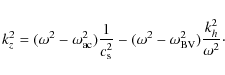
Here,
where
For vertically propagating waves (kh=0) the phase velocity is from Eq. (4)
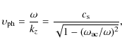
while the group velocity, with which the energy is transported, is
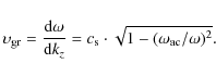
![\begin{figure}
\par\includegraphics[width=7cm,clip]{12275fig4.eps}
\end{figure}](/articles/aa/full_html/2009/47/aa12275-09/img50.png)
|
Figure 3: Transmission of solar atmosphere for acoustic waves as function of wave period with infinite spectral resolution (dashed) and after applying the convolution with spectrometer function and filtering. |
| Open with DEXTER | |
Figure 3 gives the transmission of the wave amplitudes
by the model atmosphere, i.e. the ratio of velocity amplitude,
observable as Doppler shift of the line minimum to true amplitude,
as function of period. We assume that for U = 190 s, which is close to the cutoff period, the transmission is 1. The dashed curve in Fig. 3
results for a spectrometer with infinite resolution, the solid curve is
obtained when convolving the emergent line profiles with the
spectrometer's profile and filtering in wavelength. The square of the
transmission curves as function of period (or frequency) will be used
below for correction of the velocity power. It is commonly called
the transfer function, ![]() .
The observed rms velocity at periods U shorter than the acoustic cutoff period is approximately 0.1 km s-1, thus much shorter than the thermal velocity of iron of
.
The observed rms velocity at periods U shorter than the acoustic cutoff period is approximately 0.1 km s-1, thus much shorter than the thermal velocity of iron of ![]() 1.2 km s-1,
which assures the viability of the method of calculating the
transmission. We note that for waves with periods of 50 s the wave
power in the measurement is decreased by a factor of 20, while for
a perfect spectrometer the power is decreased by a factor of 8.
On the basis of numerical simulations, Stein et al. (2004, their Fig. 9)
point out that, in addition to the signal suppression at short periods,
there is increasing radiative damping with decreasing period.
1.2 km s-1,
which assures the viability of the method of calculating the
transmission. We note that for waves with periods of 50 s the wave
power in the measurement is decreased by a factor of 20, while for
a perfect spectrometer the power is decreased by a factor of 8.
On the basis of numerical simulations, Stein et al. (2004, their Fig. 9)
point out that, in addition to the signal suppression at short periods,
there is increasing radiative damping with decreasing period.
4 Results and discussion
We now present results first from the Fourier analysis and subsequently from the wavelet analysis. The implications of the results will then be discussed in Sect. 4.3.
4.1 Fourier analysis
The temporal power spectrum from the velocity fluctuations, averaged
over the pixels in the FOV, is depicted as the dashed curve in
Fig. 4.
It shows the signatures of granular motions at around
0.5-2 mHz and of the 5-min oscillations from 2 mHz to
5 mHz and beyond. The (average) power spectra reaches the noise
level at approximately 25 mHz. The two-dimensional power
spectrum
![]() (not presented), with horizontal wave number
kh=(kx2+ky2)1/2, shows that the noise resides mainly close to kh = 0 along the frequency axis. It results from small residual jitter in the data.
(not presented), with horizontal wave number
kh=(kx2+ky2)1/2, shows that the noise resides mainly close to kh = 0 along the frequency axis. It results from small residual jitter in the data.
![\begin{figure}
\par\includegraphics[width=9cm,clip]{12275fig5.eps}
\end{figure}](/articles/aa/full_html/2009/47/aa12275-09/img53.png)
|
Figure 4:
Left panel: averaged temporal power spectra
|
| Open with DEXTER | |
We have reduced this part of the noise by applying a high-pass filter
to the three-dimensional Fourier transforms of the data. The amplitudes
were set to zero at wavelengths larger than 10
![]() .
At the same time we set also to zero the amplitudes outside the domain of propagation of acoustic waves in the
.
At the same time we set also to zero the amplitudes outside the domain of propagation of acoustic waves in the ![]() diagram, i.e. where kz2<0 and
diagram, i.e. where kz2<0 and
![]() in Eq. (4) above. The resulting temporal power spectrum is given as the solid curve in Fig. 4.
The horizontal dotted line in this figure gives our estimate of the
noise level in the high-pass filtered power spectrum. We shall restrict
the further analyses and discussion mainly to frequencies
in Eq. (4) above. The resulting temporal power spectrum is given as the solid curve in Fig. 4.
The horizontal dotted line in this figure gives our estimate of the
noise level in the high-pass filtered power spectrum. We shall restrict
the further analyses and discussion mainly to frequencies ![]() 20 mHz.
20 mHz.
After subtraction of the noise level from the power spectra we may now
estimate the acoustic flux spectra and the total flux at the layer
where the velocity signal is formed. We use the formulae
for the flux spectrum, with mass density
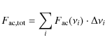
for the total acoustic flux with summation over frequency intervals
The flux spectra are shown in the right panel of Fig. 4. The thin and thick dashed curves give the spectra before and after correction for the atmospheric transmission, respectively. The thin and thick solid curves are those for the high-pass filtered data.
The dotted straight lines in the right panel of Fig. 4 indicate the frequency dependences of the acoustic flux spectra. With these we may extrapolate to higher frequencies and estimate the energy flux carried by acoustic waves with periods U<50 s (cf. Sect. 4.3).
The study of pure inter-network and network areas, as indicated in Fig. 1, gave no large difference in velocity power. We shall discuss in detail the amounts of flux below in Sect. 4.3 together with those found from the wavelet analysis. But we note here that we obtain from the high-pass filtered data flux values of 1840 W m-2 and 3190 W m-2 before and after correction, respectively.
4.2 Wavelet analysis
The temporal power spectra averaged over the FOV (cf. Fig. 4, left panel) do not show structure, apart from the signature of the 5-min oscillations. We therefore perform a wavelet analysis as in Wunnenberg et al. (2002). The code by Torrence & Compo (1988) was used with Morlet wavelets. This allows us to localise at each pixel the occurrence of velocity and intensity fluctuations along the time sequences and to determine their amplitude. We calculated the wave power in the period bands 50 s < U < 70 s, 70 s < U < 90 s, ..., up to 170 s < U < 190 s. A statistical significance level of 95% was adopted.
Figures 5 and 6
give examples of results from the wavelet analysis of velocity and
intensity at line minimum. The brightness levels indicate the square of
the fluctuation. They are inverted for better visualisation,
i.e. the darker the grey scale the more power was found. The
high-pass filtered data were used for these figures. Since filtering
requires apodisation in spatial (and temporal) coordinates, the FOV is
reduced to 20
![]() 7
7 ![]() 20
20
![]() 7.
7.
Figure 5 shows the position of power in the period range
![]() s. One sees from left to right: velocity power at a specific time t
s. One sees from left to right: velocity power at a specific time t ![]() 300 s
after the start of observation, intensity power at the same time,
velocity power averaged over time, and intensity power averaged over
time. We note from inspection of this figure and of the according full
time sequence:
300 s
after the start of observation, intensity power at the same time,
velocity power averaged over time, and intensity power averaged over
time. We note from inspection of this figure and of the according full
time sequence:
- 1.
- The power is produced in patches of
 1
1
 ,
rarely larger than 2
size. Acoustic flux appears and disappears simultaneously in the power maps of both velocity and intensity.
,
rarely larger than 2
size. Acoustic flux appears and disappears simultaneously in the power maps of both velocity and intensity.
- 2.
- The power patches last for (5
 2) min and often move horizontally with velocities of the order of 15 km s-1.
- 3.
- Velocity and intensity power maps possess similar morphology, i.e. appear to be coherent, but do not agree in detail such as in the temporal development of amplitude.
- 4.
- The power in the periods of
 s is intermittent. This agrees with the finding of Vecchio et al. (2009) from the chromospheric Ca II 8542 Å
line that shocks in this period range are abundant but occur in rare
bursts. Even after temporally averaging over the 19.2 min of the
sequence (two right panels of Fig. 5) one still has variations by a factor of 10 between minimum and maximum power in the FOV.
s is intermittent. This agrees with the finding of Vecchio et al. (2009) from the chromospheric Ca II 8542 Å
line that shocks in this period range are abundant but occur in rare
bursts. Even after temporally averaging over the 19.2 min of the
sequence (two right panels of Fig. 5) one still has variations by a factor of 10 between minimum and maximum power in the FOV.
| Figure 5:
Spatial position of power of acoustic waves in the period range 130-150 s. From left to right: velocity power at t |
|
| Open with DEXTER | |
In this period range, the signal comes from propagating acoustic waves which show, in the ![]() power spectra, the ridges of the pseudo-p-modes (cf. Krijger et al. 2001, their Fig. 23, and references therein). The horizontal phase velocity
power spectra, the ridges of the pseudo-p-modes (cf. Krijger et al. 2001, their Fig. 23, and references therein). The horizontal phase velocity
![]() of such waves can be large.
of such waves can be large.
Figure 6 exhibits power maps in the period bin
![]() s,
with velocity power in the upper row and intensity power in the lower
row. We present from left to right: power maps at
s,
with velocity power in the upper row and intensity power in the lower
row. We present from left to right: power maps at
![]() s after the start of the sequence, at
s after the start of the sequence, at
![]() s, and the temporal averages. We note from this figure and from inspection of the movies along the time sequences:
s, and the temporal averages. We note from this figure and from inspection of the movies along the time sequences:
- 1.
- The signals are very intermittent in space and time, the waves are of small scale, mostly well below 1 arcsec.
- 2.
- The power lasts often for only 2.5-4 min, i.e. not more than 2 to 3 periods.
- 3.
- We see extended patches where waves at this period bin are preferentially produced. There the velocity power reappears with large amplitude after some 5-10 min at the same or at a nearby location. The patches of the velocity wavelets are not co-spatial with network areas, cf. Fig. 1. But the wavelets from the line minimum intensity fluctuations show similarity with network structure in some cases.
- 4.
- In many cases, strong signals lasting for approximately 150 s in the velocity measurements are followed, in the same area, by similar signals in line minimum intensity fluctuation, shifted by 15-30 s and with slightly different spatio-temporal morphology.
- 5.
- The agreement between the velocity and line minimum intensity power is not as good as for the (140
10) s period bin. But the areas of power production agree coarsely.
- 6.
- In ample areas no power appears during the 19.2 min of this time sequence.
![\begin{figure}
\par\includegraphics[width=8.5cm,clip]{12275fig7.eps}
\end{figure}](/articles/aa/full_html/2009/47/aa12275-09/img67.png)
|
Figure 6:
Spatial position of power in the period bin
|
| Open with DEXTER | |
The dependence of short-period energy in the line minimum velocities on the granular convection is depicted in Fig. 7. There the counts of wavelet power for the periods 110 s < U < 190 s (solid) and 50 s < U < 110 s (dashed) vs. the normalised broadband intensity
![]()
![]()
![]()
![]() at
each position in the FOV are presented. The broadband images were taken
two time steps (=31.6 s) earlier than the wavelet powers under
analysis. This time lap corresponds approximately to the travel time
from the bottom of the photosphere to 250 km height (
at
each position in the FOV are presented. The broadband images were taken
two time steps (=31.6 s) earlier than the wavelet powers under
analysis. This time lap corresponds approximately to the travel time
from the bottom of the photosphere to 250 km height (![]() 250 km/
250 km/
![]() .
For the longer periods, we collected the positions in time and space
where the power is larger than a factor of 0.3 of the maxima in
each period band of width
.
For the longer periods, we collected the positions in time and space
where the power is larger than a factor of 0.3 of the maxima in
each period band of width ![]() = 20 s. For the shorter periods a threshold of 0.2 of the corresponding maxima was chosen.
= 20 s. For the shorter periods a threshold of 0.2 of the corresponding maxima was chosen.
| Figure 7:
Occurrence of wavelet power of velocities vs. normalised broadband intensity
|
|
| Open with DEXTER | |
Figure 7 shows clearly that the wave energy is produced predominantly in dark intergranular areas, as already found by Wunnenberg et al. (2002, their Figs. 3 and 4). We note without showing that this behaviour is present in all period bands of 20 s width, from 50 s to 190 s. Movies of granular evolution overlaid with power in various period bins confirm this finding. In addition, one also sees wavelet power occurring above small rapidly evolving granules. Wavelet power may also occur above granules before they split and above granular borders.
The results on the acoustic flux distributions averaged over time and over the total FOV, are given in Fig. 8. There we show the dependence on period U for both the uncorrected and corrected values, i.e. without division by TFi and with division.
| Figure 8: Energy flux in period bins 50-70 s, ..., 170-190 s from wavelet analysis. Dashed and asterisks: uncorrected for atmospheric transmission; solid and rhombs: corrected. |
|
| Open with DEXTER | |
The total acoustic flux is obtained, similarly as from Eqs. (8) and (9) above, by
with summation over the period intervals, and again mass density
Towards short periods, below 80 s, the corrected flux appears to increase, at least to level off at approximately 20 W m-2 s-1 (cf. Fig. 8). Taken such a constant flux level at face value and extrapolating to periods of 10 s would imply an additional acoustic flux of the order of 800 W m-2. We note that extrapolation of the flux spectra from the Fourier analysis to 100 mHz gave an additional flux of up to 400 W m-2. Thus, such an amount of flux from extrapolation is not totally improbable. Alternatively, the correction is too large. We shall expand on this point below.
4.3 Discussion
We collect the results on acoustic flux from our Fourier and wavelet analyses in Table 1
together with values given by other authors. In this table, ``IN''
and ``N'' denote inter-network and network results, respectively
and ``corr.'' indicates correction of the flux values for the
atmospheric transmission, i.e. division by ![]() (cf. Sect. 3.2). The lower limit values in italic are from application of smaller correction factors.
(cf. Sect. 3.2). The lower limit values in italic are from application of smaller correction factors.
The table contains in the rightmost column the total fluxes,
i.e. the sums over the frequency range 5.2-20 mHz. The
correction with the atmospheric transfer function ![]() is uncertain.
is uncertain. ![]() is
based on simulations of observable velocity amplitudes from waves
propagating vertically through a quiet Sun model atmosphere. We are
confident that the correction factors are reliable at frequencies below
10 mHz. But they become increasingly uncertain with increasing
frequency.
is
based on simulations of observable velocity amplitudes from waves
propagating vertically through a quiet Sun model atmosphere. We are
confident that the correction factors are reliable at frequencies below
10 mHz. But they become increasingly uncertain with increasing
frequency.
Table 1:
Energy fluxes in acoustic waves
![]() from quiet Sun disc centre. See text for meaning of ``IN'', ``N'', ``corr.'', and lower limit.
from quiet Sun disc centre. See text for meaning of ``IN'', ``N'', ``corr.'', and lower limit.
We estimated the lower limits in Table 1 of the acoustic fluxes in the various frequency bands by applying the transmission of a perfect spectrometer, i.e. the dashed transmission function in Fig. 3. The height of signal formation, h = 250 km, was not changed for the estimate. This yields, compared with the ``fully'' corrected values, a reduction by 10% in the 5.2-10 mHz band and by 40% for 10-20 mHz, and the flux from extrapolation beyond 20 mHz has become 110 W m-2.
In the wavelet analysis, we assigned half of the flux in the period bin of 90-110 s to the 5.2-10 mHz frequency band and the other half to the 10-20 mHz band. This analysis gave similar acoustic fluxes as the Fourier analysis. The values in the 5.2-10 mHz band are higher than those from the Fourier analysis by approximately 30%, while the values at 10-20 mHz are lower by 10-20%. Also here, no significant differences between inter-network and network are seen.
We discuss shortly extrapolations of the fluxes towards frequencies higher than 20 mHz. We emphasise that such extrapolated values are speculative. However, we realise that our observations both with Fourier and wavelet analysis indicate additional acoustic flux at higher frequencies. Extrapolating the slopes of the flux spectra in Fig. 4, right panel we may integrate and obtain from the Fourier analysis additional acoustic flux in the range 20-100 mHz of 10 W m-2 for the case of uncorrected fluxes. The extrapolation of the flux distribution corrected for atmospheric transmission gives additional power of 450 W m-2 and 110 W m-2 for the extrapolation in the lower limit case. For the wavelet analysis, due to lack of better observational knowledge, we extrapolate the period dependence down to 10 s with constant flux distribution using the values at the 60 s period. This gives for the uncorrected flux in the 20-100 mHz range an additional flux of 110 W m-2 and for the flux corrected for atmospheric transmission 840 W m-2. This appears to be large, but we consider it not improbable. In the lower limit case we obtain additional 380 W m-2.
Jefferies et al. (2006) have pointed
out that strong magnetic fields at the supergranular boundaries open
a ``portal'' for propagation of magnetoacoustic waves with periods
longer than the acoustic cutoff period (![]() 190 s).
This has not been accounted for in our analyses. Obviously, the
magnetic chromosphere needs more energy supply for the balance of the
radiative losses. In the present study we search for the basal energy
flux into those parts of the solar chromosphere which show very low
magnetic activity (Schrijver 1987).
190 s).
This has not been accounted for in our analyses. Obviously, the
magnetic chromosphere needs more energy supply for the balance of the
radiative losses. In the present study we search for the basal energy
flux into those parts of the solar chromosphere which show very low
magnetic activity (Schrijver 1987).
The total acoustic flux found here from velocity fluctuations amounts to ![]() 3000 W m-2 at a height of h = 250 km above
3000 W m-2 at a height of h = 250 km above ![]() = 1 in the VAL C atmospheric model (Vernazza et al. 1981).
We also find that 65-75% of the flux is carried by waves with
frequencies of 5.2-10 mHz and 25-30% by waves with higher
frequencies. Wunnenberg et al. (2002)
measured, also in a wavelet analysis, yet without correction for
atmospheric transmission, an acoustic flux of 900 W m-2 in the period range 7.7-20 mHz at
= 1 in the VAL C atmospheric model (Vernazza et al. 1981).
We also find that 65-75% of the flux is carried by waves with
frequencies of 5.2-10 mHz and 25-30% by waves with higher
frequencies. Wunnenberg et al. (2002)
measured, also in a wavelet analysis, yet without correction for
atmospheric transmission, an acoustic flux of 900 W m-2 in the period range 7.7-20 mHz at
![]() km.
The total flux from the present study is higher by a factor of
approximately 2 than the value of 1400 W m-2 given by Straus et al. (2008)
at the same atmospheric height. This latter value is not corrected for
atmospheric transmission. It is somewhat lower than the 1850 and
2500 W m-2 for our uncorrected measurements from
Fourier and wavelet analysis, respectively. We speculate that the
spatial resolution in the present work is somewhat higher than in the
data used by Straus et al. According to the numerical simulations
by Straus et al. (2008), the flux would decrease by
km.
The total flux from the present study is higher by a factor of
approximately 2 than the value of 1400 W m-2 given by Straus et al. (2008)
at the same atmospheric height. This latter value is not corrected for
atmospheric transmission. It is somewhat lower than the 1850 and
2500 W m-2 for our uncorrected measurements from
Fourier and wavelet analysis, respectively. We speculate that the
spatial resolution in the present work is somewhat higher than in the
data used by Straus et al. According to the numerical simulations
by Straus et al. (2008), the flux would decrease by ![]() 30% before reaching the base of the average chromosphere at
30% before reaching the base of the average chromosphere at
![]() km due to radiative damping. Yet the actual reduction is again uncertain (cf. Fig. 3 in Straus et al. 2008). The high frequency waves are the most prone to damping (Stein et al. 2004). Also, it is important to note that the flux measurements by Straus et al. (2008)
are in excellent agreement with the results of their numerical
simulations. This underlines the needs for further work in this field,
combining high-resolution observations with sophisticated numerical
simulations.
km due to radiative damping. Yet the actual reduction is again uncertain (cf. Fig. 3 in Straus et al. 2008). The high frequency waves are the most prone to damping (Stein et al. 2004). Also, it is important to note that the flux measurements by Straus et al. (2008)
are in excellent agreement with the results of their numerical
simulations. This underlines the needs for further work in this field,
combining high-resolution observations with sophisticated numerical
simulations.
An interesting new finding on energy flux carried by atmospheric gravity waves was reported by Straus et al. (2008). They give a flux of 20 800 W m-2 at h = 250 km, which is reduced to ![]() 5000 W m-2 at h =
500 km, an amount of energy supply to account for the heating of
atmospheric layers above that height to a ``warm'' chromosphere
from which UV emission lines would be observed. Vernazza et al. (1981) give radiative losses of 4600 W m-2 for their model C, while Anderson & Athay (1989) quote 14 000 W m-2 when including radiative losses from Fe II lines.
5000 W m-2 at h =
500 km, an amount of energy supply to account for the heating of
atmospheric layers above that height to a ``warm'' chromosphere
from which UV emission lines would be observed. Vernazza et al. (1981) give radiative losses of 4600 W m-2 for their model C, while Anderson & Athay (1989) quote 14 000 W m-2 when including radiative losses from Fe II lines.
The energy flux in acoustic waves found by Fossum & Carlsson (2006) from intensity fluctuations in TRACE filtergram time sequences is much below the flux found here, by a factor of 6, at least by a factor of 4 when accounting for possible wave damping for our result at h=250 km. Likewise, the measurement of intensity fluctuations with high-spatial resolution from HINODE filtergram time series in Ca II H by Carlsson et al. (2007) gave acoustic fluxes lower than a factor of 3-4 than our result. We suggest that the TRACE data have not sufficient spatial resolution to detect more short-period waves, while the HINODE filtergrams in Ca II H measure over a too extended height range.
5 Conclusions
We have analysed a time series of two-dimensional (2D) narrowband spectrograms in the non-magnetic Fe I 5576 Å line. The sequence had a duration of ![]() 22 min
and a cadence of 15.8 s. The data were reconstructed with speckle
methods. Intensity and velocity fluctuations at line minimum have been
determined, and the velocities were corrected for the transmission of
the solar atmosphere. The 2D data sets were subjected to Fourier
and wavelet analyses. We obtained energy fluxes carried by waves with
frequencies above the acoustic cutoff frequency (
22 min
and a cadence of 15.8 s. The data were reconstructed with speckle
methods. Intensity and velocity fluctuations at line minimum have been
determined, and the velocities were corrected for the transmission of
the solar atmosphere. The 2D data sets were subjected to Fourier
and wavelet analyses. We obtained energy fluxes carried by waves with
frequencies above the acoustic cutoff frequency (![]() 5.2 mHz) at a height of
5.2 mHz) at a height of ![]() 250 km in the solar atmosphere. We summarise the results as follows:
250 km in the solar atmosphere. We summarise the results as follows:
- 1.
- Both Fourier and wavelet analysis give total acoustic fluxes
 of 2600-3600 W m-2
at 250 km in the solar atmosphere. 65-75% of this flux is carried
by waves in the frequency range 5.2-10 mHz, and 25-35% by waves at
higher frequencies.
of 2600-3600 W m-2
at 250 km in the solar atmosphere. 65-75% of this flux is carried
by waves in the frequency range 5.2-10 mHz, and 25-35% by waves at
higher frequencies. - 2.
- The waves appear in small-scale areas, of 1
-2
size for waves in the band of longer periods and at scales definitely below 1
in the short-period band. In the whole analysed period range from
50 s to 190 s, the power occurs predominantly above
inter-granular areas.
- 3.
- We do not see a large difference between the fluxes in pure inter-network areas and those in network.
The finding that much of the flux is carried in the frequency band 5.2-10 mHz, i.e. at periods shorter than the acoustic cutoff period at 190 s down to 100 s, supports the conjecture by Reardon et al. (2008). These authors suggest that the chromospheric power spectra measured by them in Ca II 8542 is a result from shock dissipation of waves near the cutoff frequency. We speculate that the mechanical flux of 1800-2500 W m-2 carried by acoustic waves to the chromosphere can serve, together with the flux in atmospheric gravity waves of 5000 W m-2 found by Straus et al. (2008), to produce at least a ``warm'' chromosphere, on average. This would then be the amount of basal flux to balance the radiative losses from chromospheric parts with little magnetic field (Schrijver 1987).
Our finding of most acoustic energy flux in the 5.2-10 mHz range seemingly supports the view that waves with periods U < 50 s are unimportant (e.g. Stein et al. 2004). Yet we emphasise that, from the observational point of view, we find many uncertainties in the frequency or period distribution of acoustic flux in the photosphere. Our knowledge is insufficient due to limited angular resolution and limited resolution in atmospheric height. Thus, we consider the problem of chromospheric heating not yet solved satisfactorily. Its solution is important because the chromospheres of the Sun and of late-type stars are the layers of the onset of exchange of mass, momentum, and energy between the stellar interior and the heliosphere and the interstellar medium.
To answer the question on chromospheric energy supply one would
like to perform an observational experiment with high spatial
resolution, much better than 0
![]() 5,
with high cadence, of the order of 10 s, with very good
discrimination in height, and with low noise. Possibly, a combination
of signals originating from various heights will allow us to narrow the
height ranges of signal formation. A multi-line capability would
be very valuable to follow the wave propagation in various atmospheric
heights. The next generation of detectors and data acquisition systems
will certainly lead to high-cadence measurements. To achieve high
spatial resolution and obtain simultaneously low-noise data is a task
for telescopes with large aperture, such as GREGOR, EST, and ATST,
including high-order Adaptive Optics. At the same time, such
observations and their interpretation need to be guided by numerical
simulations, as in Stein et al. (2004), Wedemeyer-Böhm et al. (2007), Straus et al. (2008), and most recently for photospheric magnetic field dynamics in Bello González et al. (2009). High Reynolds numbers are much desirable as well as small grid sizes in (x,y,z,t).
The goal would be to model the process of wave generation from
turbulence and to follow their propagation through the solar
atmosphere.
5,
with high cadence, of the order of 10 s, with very good
discrimination in height, and with low noise. Possibly, a combination
of signals originating from various heights will allow us to narrow the
height ranges of signal formation. A multi-line capability would
be very valuable to follow the wave propagation in various atmospheric
heights. The next generation of detectors and data acquisition systems
will certainly lead to high-cadence measurements. To achieve high
spatial resolution and obtain simultaneously low-noise data is a task
for telescopes with large aperture, such as GREGOR, EST, and ATST,
including high-order Adaptive Optics. At the same time, such
observations and their interpretation need to be guided by numerical
simulations, as in Stein et al. (2004), Wedemeyer-Böhm et al. (2007), Straus et al. (2008), and most recently for photospheric magnetic field dynamics in Bello González et al. (2009). High Reynolds numbers are much desirable as well as small grid sizes in (x,y,z,t).
The goal would be to model the process of wave generation from
turbulence and to follow their propagation through the solar
atmosphere.
N.B.G. acknowledges financial support by Deutsche Forschungsgemeinschaft through grants KN 152/29-3 and KN 152/31-1. M.F.S. was supported by the ERASMUS programme of the European Union. O.O. thanks for support by Deutsche Forschungsgemeinschaft through grant KN 152/29-3 and by the Institut für Astrophysik of the Georg-August-Universität Göttingen. The Vacuum Tower Telescope is operated by the Kiepenheuer-Institut für Sonnenphysik, Freiburg, at the Spanish Observatorio del Teide of the Instituto de Astrofísica de Canarias. Wavelet software was provided by C. Torrence and G. Compo, and is available at URL: http://paos.colorado.edu/research/wavelets.
Appendix A: Influence of pre-filter and noise filter
We describe in this Appendix the influence of the rather broad pre-filter with 11 Å FWHM and of the applied wavelength filter to smooth the line profiles. Figure A.1
depicts a 22 Å wide section of the solar spectrum from the
Fourier Transform Spectrometer Atlas (FTS, Brault & Neckel, quoted
by Neckel 1999). We adopt that the broadening
of the spectral lines by the FTS is negligible, i.e. the FTS has
an infinite spectral resolution. The transmission of the pre-filter,
taken from the data sheet of the manufacturer, normalised to its
maximum, is shown as the dotted curve. The solar spectrum multiplied
with the transmission of the pre-filter gives the input to the
Fabry-Perot interferometer (FPI). The transmission of the latter, also
normalised to its maximum, is the dashed curve with the ordinate on the
right side of Fig. A.1. We take finesses of
![]() for both etalons with plate spacings of 1.101 mm and 1.408 mm
and a neutral density filter between the etalons of 30% absorption
(Bello González & Kneer 2008, Sect. 2.1 there).
for both etalons with plate spacings of 1.101 mm and 1.408 mm
and a neutral density filter between the etalons of 30% absorption
(Bello González & Kneer 2008, Sect. 2.1 there).
![\begin{figure}
\par\includegraphics[width=8.5cm,clip]{12275fig10.eps}
\end{figure}](/articles/aa/full_html/2009/47/aa12275-09/img79.png)
|
Figure A.1:
Solid: section of the solar spectrum from the Fourier Transform Spectrometer Atlas (FTS, Brault & Neckel, quoted by Neckel 1999); dotted: transmission of the pre-filter with |
| Open with DEXTER | |
One sees in the section of the solar spectrum several moderately strong
to strong spectral lines whose positions are close to the transmission
peaks of the FPI and whose intensities are not fully suppressed by the
pre-filter. While scanning, i.e. moving the FPI transmission
across the input by
![]() 0.25 Å, these lines can have an influence on the velocity measurements of the Fe I 5576 Å line: an unidentified line (according to Moore et al. 1966)
at 5566.1 Å at a 1% level relative to the
5576 Å line (FPI transmission multiplied with the
transmission of the pre-filter), the Fe I 5582.0 Å line at a 0.5% level, and the four Fe I lines at 5576.4 Å, 5569.6 Å, 5572.9 Å, 5573.1 Å plus the Ni I line
at 5578.7 Å. The influence of these latter five lines sums up to a
level of 0.5% relative to the 5576 Å line. The total amount
of false line shifts from the above lines is thus at the 2% level.
Tests were performed by shifting the whole solar spectrum, except the
central part around 5576 Å, corresponding to a velocity of
1 km s-1. The resulting, false line shift in 5576 corresponded to 26 m s-1. We thus may neglect the shifts induced by the broad pre-filter.
0.25 Å, these lines can have an influence on the velocity measurements of the Fe I 5576 Å line: an unidentified line (according to Moore et al. 1966)
at 5566.1 Å at a 1% level relative to the
5576 Å line (FPI transmission multiplied with the
transmission of the pre-filter), the Fe I 5582.0 Å line at a 0.5% level, and the four Fe I lines at 5576.4 Å, 5569.6 Å, 5572.9 Å, 5573.1 Å plus the Ni I line
at 5578.7 Å. The influence of these latter five lines sums up to a
level of 0.5% relative to the 5576 Å line. The total amount
of false line shifts from the above lines is thus at the 2% level.
Tests were performed by shifting the whole solar spectrum, except the
central part around 5576 Å, corresponding to a velocity of
1 km s-1. The resulting, false line shift in 5576 corresponded to 26 m s-1. We thus may neglect the shifts induced by the broad pre-filter.
![\begin{figure}
\par\includegraphics[width=8.5cm,clip]{12275fig11.eps}
\end{figure}](/articles/aa/full_html/2009/47/aa12275-09/img81.png)
|
Figure A.2: Dashed: section of spectrum from FTS around Fe I 5576 line; solid: same section after convolution with FPI transmission; dotted: line spread function of 49 mÅ FWHM for smoothing in wavelength; asterisks: line profile with observational wavelength spacing after smoothing in wavelength. |
| Open with DEXTER | |
The influence of the broad pre-filter on the profile of Fe I 5576 Å is shown in Fig. A.2. There, the dashed profile is from the FTS atlas and the solid profile the FTS profile multiplied with the transmission of the pre-filter, then convolved with the FPI transmission and finally normalised to maximum intensity along the spectrum. One sees that the residual intensity of the convolved profile has increased by approximately a factor of two, as found above (Fig. 2 and Eq. (1) in Sect. 3.1).
For a precise measurement of the Doppler shifts we reduced the noise and the fluctuations of spectrometer transmission on short wavelength scales (cf. Bello González & Kneer 2008, Sect. 2.1). For this we applied a filter whose Fourier transform is shown as the line spread function (LSP) by the dotted line in Fig. A.2. The LSP has an FWHM of 49 mÅ. It preserves well the general shape of the line profile. Thus, the finally measured line intensities, indicated by the asterisks in Fig. A.2 do almost not differ from the original (though convolved with the FPI transmission) profiles. But the filter mixes intensities from the line wings to the line centre and vice versa. The result is a lowering of the formation height of the velocity fluctuations and a broadening (in height) of the velocity response function.
References
- Anderson, L. S., & Athay, R. G. 1989, ApJ, 346, 1010 [NASA ADS] [CrossRef]
- Bello González, N., & Kneer, F. 2008, A&A, 480, 265 [NASA ADS] [EDP Sciences] [CrossRef]
- Bello González, N., Okunev, O. V., Domínguez Cerdeña, I., Kneer, F., & Puschmann, K. G. 2005, A&A, 434, 317 [NASA ADS] [EDP Sciences] [CrossRef]
- Bello González, N., Kneer, F., & Puschmann, K. G. 2007, in Modern Solar Facilities - Advanced Solar Science, ed. F. Kneer, K. G. Puschmann, & A. D. Wittmann, Universitätsverlag Göttingen, 217
- Bello González, N., Yelles Chaouche, L., Okunev, O., & Kneer, F. 2009, A&A, 494, 1091 [NASA ADS] [EDP Sciences] [CrossRef]
- Bendlin, C., & Volkmer, R. 1995, A&AS, 112, 371 [NASA ADS]
- Bendlin, C., Volkmer, R., & Kneer, F. 1992, A&A, 257, 817 [NASA ADS]
- Biermann, L. 1948, ZAp, 25, 161 [NASA ADS]
- Carlsson, M., & Stein, R. F. 1995, ApJ, 440, L29 [NASA ADS] [CrossRef]
- Carlsson, M., & Stein, R. F. 1997, ApJ, 481, 500 [NASA ADS] [CrossRef]
- Carlsson, M., Judge, P. G., & Wilhelm, K. 1997, ApJ, 486, L63 [NASA ADS] [CrossRef]
- Carlsson, M., Hansteen, V. H., De Pontieu, B., et al. 2007, PASJ, 59, 663 [NASA ADS]
- Cuntz, M., Rammacher, W., & Musielak, Z. E. 2007, ApJ, 657, L57 [NASA ADS] [CrossRef]
- Cram, L. E., Keil, S. L., & Ulmschneider, P. 1979, ApJ, 234, 768 [NASA ADS] [CrossRef]
- de Boer, C. R. 1996, A&AS, 120, 195 [NASA ADS] [EDP Sciences] [CrossRef]
- Durrant, C. J. 1979, A&A, 73, 137 [NASA ADS]
- Eibe, M. T., Mein, P., Roudier, Th., & Faurobert, M. 2001, A&A, 371, 1128 [NASA ADS] [EDP Sciences] [CrossRef]
- Fawzy, D., Rammacher, W., Ulmschneider, P., Musielak, Z. E., & Stepien, K. 2002, A&A, 386, 971 [NASA ADS] [EDP Sciences] [CrossRef]
- Fossum, A., & Carlsson, M. 2005a, ApJ, 625, 556 [NASA ADS] [CrossRef]
- Fossum, A., & Carlsson, M. 2005b, Nature, 435, 919 [NASA ADS] [CrossRef]
- Fossum, A., & Carlsson, M. 2006, ApJ, 646, 579 [NASA ADS] [CrossRef]
- Handy, B. N. Acton, L. W., Krankelborg, C. C., et al. 1999, Sol. Phys., 187, 229 [NASA ADS] [CrossRef]
- Hasan, S. S., & van Ballegooijen, A. A. 2008, ApJ, 680, 1542 [NASA ADS] [CrossRef]
- Hasan, S. S., van Ballegooijen, A. A., Kalkofen, W., & Steiner, O. 2005, ApJ, 631, 1270 [NASA ADS] [CrossRef]
- Jefferies, S. M., McIntosh, S. W., Armstrong, J. D., et al. 2006, ApJ, 648, L151 [NASA ADS] [CrossRef]
- Kalkofen, W., Ulmschneider, P., & Avrett, E. H. 1999, ApJ, 521, L141 [NASA ADS] [CrossRef]
- Keller, C. U., & von der Lühe, O. 1992, A&A, 261, 321 [NASA ADS]
- Krieg, J., Wunnenberg, M., Kneer, F., Koschinsky, M., & Ritter, C. 1999, A&A, 343, 983 [NASA ADS]
- Krijger, J. M., Rutten, R. J., Lites, B. W., et al. 2001, A&A, 379, 1052 [NASA ADS] [EDP Sciences] [CrossRef]
- Lighthill, M. J. 1952, Proc. Roy. Soc. London, A211, 564 [NASA ADS]
- Maltby, P., Avrett, E. H., Carlsson, M., et al. 1986, ApJ, 306, 284 [NASA ADS] [CrossRef]
- Mein, N., & Mein, P. 1980, A&A, 84, 96 [NASA ADS]
- Mein, P. 1971, Sol. Phys., 20, 3 [NASA ADS] [CrossRef]
- Moore, C. E., Minnaert, M. G. J., & Houtgast, J. 1966, The Solar Spectrum 2935 Å to 8770 Å, NBS, Monograph, 61
- Musielak, Z. E., & Ulmschneider, P. 2003a, A&A, 400, 1057 [NASA ADS] [EDP Sciences] [CrossRef]
- Musielak, Z. E., & Ulmschneider, P. 2003b, A&A, 406, 725 [NASA ADS] [EDP Sciences] [CrossRef]
- Neckel, H. 1999, Sol. Phys., 184, 421 [CrossRef]
- Puschmann, K. G., Kneer, F., Seelemann, T., & Wittmann, A. D. 2006, A&A, 445, 337 [NASA ADS] [EDP Sciences] [CrossRef]
- Reardon, K. P., & Cavallini, F. 2008, A&A, 481, 897 [NASA ADS] [EDP Sciences] [CrossRef]
- Reardon, K. P., Lepreti, F., Carbone, V., & Vecchio, A. 2008, ApJ, 683, L207 [NASA ADS] [CrossRef]
- Schrijver, C. J. 1987, A&A, 172, 111 [NASA ADS]
- Schwarzschild, M. 1948, ApJ, 107, 1 [NASA ADS] [CrossRef]
- Shchukina, N., & Trujillo Bueno, J. 2001, ApJ, 550, 970 [NASA ADS] [CrossRef]
- Stein, R. F. 1967, Sol. Phys., 2, 385 [NASA ADS] [CrossRef]
- Stein, R. F., Bogdan, T. J., Carlsson, M., et al. 2004, in SOHO 13 - Waves, Oscillations and Small-Scale Transient Events in the Solar Atmosphere: A Joint View from SOHO and TRACE, ed. H. Lacoste, ESA SP-457, 93
- Straus, T., Fleck, B., Jefferies, S. M., et al. 2008, ApJ, 681, L125 [NASA ADS] [CrossRef]
- Torrence, C., & Compo, G. P. 1998, Bull. Amer. Meteor. Soc., 79, 61 [CrossRef]
- Tsuneta, S., Ichimoto, K., Katsukawa, Y., et al. 2008, Sol. Phys., 249, 167 [NASA ADS] [CrossRef]
- Ulmschneider, P., Rammacher, W., Musielak, Z. E., & Kalkofen, W. 2005, ApJ, 631, L155 [NASA ADS] [CrossRef]
- Vecchio, A., Cauzzi, G., Reardon, K. P., Janssen, K., & Rimmele, T. 2007, A&A, 461, L1 [NASA ADS] [EDP Sciences] [CrossRef]
- Vecchio, A., Cauzzi, G., & Reardon, K. P. 2009, A&A, 494, 269 [NASA ADS] [EDP Sciences] [CrossRef]
- Vernazza, J. E., Avrett, E. H., & Loeser, R. 1981, ApJS, 45, 635 [NASA ADS] [CrossRef]
- Volkmer, R., Kneer, F., & Bendlin, C. 1995, A&A, 304, L1 [NASA ADS]
- von der Lühe, O. 1984, J. Opt. Soc. Am. A1, 510
- von der Lühe, O., Soltau, D., Berkefeld, T., & Schelenz, T. 2003, SPIE, 4853, 187 [NASA ADS]
- Wedemeyer-Böhm, S., Steiner, O., Bruls, J., & Rammacher, W. 2007, in The Physics of Chromospheric Plasmas, ed. I. Dorotovic, P. Heinzel, & R. Rutten, ASP Conf. Ser., 368, 93
- Weigelt, G. P. 1977, Opt. Comm., 21, 55 [NASA ADS] [CrossRef]
- Wunnenberg, M., Kneer, F., & Hirzberger, J. 2002, A&A, 395, L1 [NASA ADS] [EDP Sciences] [CrossRef]
- Yi, Z., & Molowny Horas, R. L. 1992, in Proc. from LEST Mini-Workshop, Software for Solar Image Processing, ed. Z. Yi, T. Darvann, & R. Molowny Horas, Oslo, Institute of Theoretical Astrophysics, 69
All Tables
Table 1:
Energy fluxes in acoustic waves
![]() from quiet Sun disc centre. See text for meaning of ``IN'', ``N'', ``corr.'', and lower limit.
from quiet Sun disc centre. See text for meaning of ``IN'', ``N'', ``corr.'', and lower limit.
All Figures
|
|
Figure 1: From time series in Fe I 5576 Å line, clockwise starting at upper left: broadband image, minimum intensity, minimum intensity averaged over time sequence, and velocity from minimum position of line with bright indicating upward flow. The boxes with ``N'' and ``IN'' indicate network and inter-network areas, respectively. Axes are in arcsec. The dark patches in the velocity map ( lower left) at positions (20, 10) and (7, 15), result from the coincidence of intergranular down-flow and the downwards motions from the 5-min osciallations. |
| Open with DEXTER | |
| In the text | |
|
|
Figure 2:
Upper panel: response functions for velocity
|
| Open with DEXTER | |
| In the text | |
|
|
Figure 3: Transmission of solar atmosphere for acoustic waves as function of wave period with infinite spectral resolution (dashed) and after applying the convolution with spectrometer function and filtering. |
| Open with DEXTER | |
| In the text | |
|
|
Figure 4:
Left panel: averaged temporal power spectra
|
| Open with DEXTER | |
| In the text | |
| |
Figure 5:
Spatial position of power of acoustic waves in the period range 130-150 s. From left to right: velocity power at t |
| Open with DEXTER | |
| In the text | |
|
|
Figure 6:
Spatial position of power in the period bin
|
| Open with DEXTER | |
| In the text | |
| |
Figure 7:
Occurrence of wavelet power of velocities vs. normalised broadband intensity
|
| Open with DEXTER | |
| In the text | |
| |
Figure 8: Energy flux in period bins 50-70 s, ..., 170-190 s from wavelet analysis. Dashed and asterisks: uncorrected for atmospheric transmission; solid and rhombs: corrected. |
| Open with DEXTER | |
| In the text | |
|
|
Figure A.1:
Solid: section of the solar spectrum from the Fourier Transform Spectrometer Atlas (FTS, Brault & Neckel, quoted by Neckel 1999); dotted: transmission of the pre-filter with |
| Open with DEXTER | |
| In the text | |
|
|
Figure A.2: Dashed: section of spectrum from FTS around Fe I 5576 line; solid: same section after convolution with FPI transmission; dotted: line spread function of 49 mÅ FWHM for smoothing in wavelength; asterisks: line profile with observational wavelength spacing after smoothing in wavelength. |
| Open with DEXTER | |
| In the text | |
Copyright ESO 2009
Current usage metrics show cumulative count of Article Views (full-text article views including HTML views, PDF and ePub downloads, according to the available data) and Abstracts Views on Vision4Press platform.
Data correspond to usage on the plateform after 2015. The current usage metrics is available 48-96 hours after online publication and is updated daily on week days.
Initial download of the metrics may take a while.