| Issue |
A&A
Volume 508, Number 1, December II 2009
|
|
|---|---|---|
| Page(s) | 141 - 160 | |
| Section | Extragalactic astronomy | |
| DOI | https://doi.org/10.1051/0004-6361/200912884 | |
| Published online | 08 October 2009 | |
A&A 508, 141-160 (2009)
On the abundance of gravitational arcs produced by submillimeter galaxies at radio and submm wavelengths
C. Fedeli1,2,3 - A. Berciano Alba4,5
1 - Dipartimento di Astronomia, Università di Bologna, via Ranzani 1, 40127 Bologna, Italy
2 - INAF - Osservatorio Astronomico di Bologna, via Ranzani 1, 40127 Bologna, Italy
3 - INFN, Sezione di Bologna, Viale Berti Pichat 6/2, 40127 Bologna, Italy
4 - Netherlands Institute for Radio Astronomy, Postbus 2, 7990 AA, Dwingeloo, The Netherlands
5 - Kapteyn Astronomical Institute, University of Groningen, PO Box 800, 9700 AV, Groningen,
The Netherlands
Received 14 July 2009 / Accepted 7 September 2009
Abstract
We predict the abundance of giant gravitational arcs produced by
submillimeter galaxies (SMGs) lensed by foreground galaxy clusters,
both at radio and submm wavelengths. The galaxy cluster
population is modeled in a realistic way with the use of semi-analytic
merger trees, while the density profiles of individual deflectors take
into account ellipticity and substructures. The adopted typical size of
the radio and submm emitting regions of SMGs is based on current
radio/CO observations and the FIR-radio correlation. The source
redshift distribution has been
modeled using three different functions (based on
spectroscopic/photometric redshift measurements and a simple
evolutionary model) to quantify the effect of a high redshift tail on
the number of arcs. The source number counts are compatible with
currently available observations, and were suitably distorted to take
into account the lensing magnification bias. We present tables and
plots for the numbers of radio and submm arcs produced by SMGs as a
function of surface brightness, useful for the planning of future
surveys aimed at arc statistics studies. They show that e.g., the
detection of several hundred submm arcs on the whole sky with a
signal-to-noise ratio of at least 5 requires a sensitivity of
1 mJy arcsec-2 at ![]() m.
Approximately the same number of radio arcs should be detected with the
same signal-to-noise ratio with a surface brightness threshold of
m.
Approximately the same number of radio arcs should be detected with the
same signal-to-noise ratio with a surface brightness threshold of ![]() Jy arcsec-2 at 1.4 GHz. Comparisons of these results with previous work found in the literature are also discussed.
Jy arcsec-2 at 1.4 GHz. Comparisons of these results with previous work found in the literature are also discussed.
Key words: gravitational lensing - galaxies: clusters: general - radio continuum: galaxies - submillimeter
1 Introduction
The effect of gravitational lensing constitutes a unique research tool
in many astrophysical fields, since it allows one to investigate the
structures of both the lenses (e.g., galaxies and galaxy clusters) and
the lensed background sources, as well as to probe the
three-dimensional mass distribution of the Universe. In particular, one
of the most spectacular phenomena associated with
the gravitational deflection of light are the giant arcs observed in
galaxy clusters, which are caused by extended background sources lying
in the regions where the lensing magnification produced by the cluster
is strongest. The effective source magnification can easily reach ![]() in
these cases, providing the opportunity to detect and spatially resolve
the morphologies and internal dynamics of high redshift background
sources at a level of detail far greater than otherwise possible.
An illustration of this powerful technique was presented in Swinbank et al. (2007),
where a magnification factor of 16 by the
cluster RCS 0224-002 allowed them to study the star formation
activity, mass and feedback processes of a Lyman break galaxy at
in
these cases, providing the opportunity to detect and spatially resolve
the morphologies and internal dynamics of high redshift background
sources at a level of detail far greater than otherwise possible.
An illustration of this powerful technique was presented in Swinbank et al. (2007),
where a magnification factor of 16 by the
cluster RCS 0224-002 allowed them to study the star formation
activity, mass and feedback processes of a Lyman break galaxy at ![]() ,
something that
(without the help of lensing) would not be possible beyond
,
something that
(without the help of lensing) would not be possible beyond ![]() with current instruments.
with current instruments.
A particularly interesting application of gravitational lensing is the so-called arc statistics, i.e. the study of the abundance of large tangential arcs in galaxy clusters. Among other things, this abundance is sensitive to the cluster mass function, the cluster dynamical activity (e.g., infall of matter, mergers, etc.) and internal structure of host dark-matter halos (e.g., triaxiality and the concentration of the density profile), which makes arc statistics a unique tool to study the cluster population. Arc statistics studies at optical and near-infrared wavelengths have been numerous in the past decade on both the observational (Gladders et al. 2003; Luppino et al. 1999; Zaritsky & Gonzalez 2003) and theoretical sides (Wambsganss et al. 2005; Bartelmann & Weiss 1994; Fedeli et al. 2008; Meneghetti et al. 2003; Wambsganss et al. 1998; Bartelmann et al. 2003).
All the currently known giant arcs come from detections in the optical.
However, the fraction of lensed sources observed in the mm/submm
wavebands is expected to be much larger than in the optical
(Blain 1997,1996):
Due to the spectral shape of the thermal dust emission, the observed
submm flux density of dusty galaxies with a given luminosity
remains approximately constant in the redshift range
![]() instead of declining with increasing distance (usually referred to as ``negative K-correction'', see Blain & Longair 1993,1996; Blain et al. 2002).
This effect, together with the steep slope of the observed submm number
counts, produces a strong magnification bias that makes submm galaxies
(hereafter SMGs) an ideal source population for the production of
lensed arcs.
instead of declining with increasing distance (usually referred to as ``negative K-correction'', see Blain & Longair 1993,1996; Blain et al. 2002).
This effect, together with the steep slope of the observed submm number
counts, produces a strong magnification bias that makes submm galaxies
(hereafter SMGs) an ideal source population for the production of
lensed arcs.
The SMGs were first detected about a decade ago with SCUBA![]() (Barger et al. 1998; Smail et al. 1997; Eales et al. 1999; Hughes et al. 1998).
The current observational evidence indicates that these objects are
high-redshift dust obscured galaxies, in which the rest frame
FIR peak of emission is observed in the submm band. Their
FIR luminosities, in the range
(Barger et al. 1998; Smail et al. 1997; Eales et al. 1999; Hughes et al. 1998).
The current observational evidence indicates that these objects are
high-redshift dust obscured galaxies, in which the rest frame
FIR peak of emission is observed in the submm band. Their
FIR luminosities, in the range
![]() ,
are
,
are ![]() times
higher than what is observed in local spirals. Their energy output
seems to be dominated by star formation processes induced by galaxy
interactions/mergers, although a good fraction (
times
higher than what is observed in local spirals. Their energy output
seems to be dominated by star formation processes induced by galaxy
interactions/mergers, although a good fraction (
![]() )
of SMGs also seems to host an Active Galactic Nucleus (AGN, e.g. Michaowski et al. 2009; Alexander et al. 2005). The available evidence also suggests that SMGs might be the progenitors of massive local ellipticals (Webb et al. 2003; Smail et al. 2004; Alexander et al. 2003; Genzel et al. 2003; Alexander et al. 2005; Smail et al. 2002; Lilly et al. 1999; Michaowski et al. 2009; Swinbank et al. 2006,2008).
)
of SMGs also seems to host an Active Galactic Nucleus (AGN, e.g. Michaowski et al. 2009; Alexander et al. 2005). The available evidence also suggests that SMGs might be the progenitors of massive local ellipticals (Webb et al. 2003; Smail et al. 2004; Alexander et al. 2003; Genzel et al. 2003; Alexander et al. 2005; Smail et al. 2002; Lilly et al. 1999; Michaowski et al. 2009; Swinbank et al. 2006,2008).
In the ![]() clusters observed with SCUBA (Knudsen et al. 2008; Chapman et al. 2002; Cowie et al. 2002; Smail et al. 2002), only 4 multiply imaged SMGs have been reported to date (Knudsen et al. 2008; Borys et al. 2004; Kneib et al. 2004). This extremely low detection rate is due to three major limitations of current
clusters observed with SCUBA (Knudsen et al. 2008; Chapman et al. 2002; Cowie et al. 2002; Smail et al. 2002), only 4 multiply imaged SMGs have been reported to date (Knudsen et al. 2008; Borys et al. 2004; Kneib et al. 2004). This extremely low detection rate is due to three major limitations of current ![]() m surveys: (i) very small sky coverage (
m surveys: (i) very small sky coverage (![]() square degrees, including all cluster and blank field surveys); (ii) confusion limited maps at
square degrees, including all cluster and blank field surveys); (ii) confusion limited maps at ![]() mJy (which means that only the brightest members are detected) and (iii) insufficient resolution (
mJy (which means that only the brightest members are detected) and (iii) insufficient resolution (
![]() )
to resolve extended lensed structures. Current
efforts to increase the surveyed area at 850
)
to resolve extended lensed structures. Current
efforts to increase the surveyed area at 850 ![]() m include the SASS
m include the SASS![]() , the SCLS
, the SCLS![]() and the all sky survey that will be carried out with the HFI bolometer on board of the Planck
satellite
and the all sky survey that will be carried out with the HFI bolometer on board of the Planck
satellite![]() , but their resolutions will still be insufficient to identify lensed arcs. The only instrument that can
currently provide sub-arcsecond resolution in submm (at
, but their resolutions will still be insufficient to identify lensed arcs. The only instrument that can
currently provide sub-arcsecond resolution in submm (at ![]() m) is the SMA
m) is the SMA![]() .
.
However, the tight correlation between radio synchrotron and FIR emission observed in star-forming galaxies (van der Kruit 1973; Helou et al. 1985),
provides an alternative way to obtain high resolution images
of SMGs. Commonly referred to as ``the FIR/radio correlation'', it
covers about five orders of magnitude in luminosity (Garrett 2002; Condon 1992) out to ![]() (Vlahakis et al. 2007; Kovács et al. 2006; Michaowski et al. 2009; Ibar et al. 2008).
The standard model about its nature considers that both emissions are
caused by massive star formation: while young massive stars produce
UV radiation that is re-emitted in the FIR by the surrounding
dust, old massive stars explode as supernovae, producing electrons that
are accelerated by the galactic magnetic field and generate the
observed radio synchrotron emission (Harwit & Pacini 1975; Helou et al. 1985).
Therefore, given the possible common physical origin of both emissions,
radio interferometric observations can be used as a high-resolution
proxy for the rest-frame FIR emission
of high-z galaxies observed in the submm.
(Vlahakis et al. 2007; Kovács et al. 2006; Michaowski et al. 2009; Ibar et al. 2008).
The standard model about its nature considers that both emissions are
caused by massive star formation: while young massive stars produce
UV radiation that is re-emitted in the FIR by the surrounding
dust, old massive stars explode as supernovae, producing electrons that
are accelerated by the galactic magnetic field and generate the
observed radio synchrotron emission (Harwit & Pacini 1975; Helou et al. 1985).
Therefore, given the possible common physical origin of both emissions,
radio interferometric observations can be used as a high-resolution
proxy for the rest-frame FIR emission
of high-z galaxies observed in the submm.
The advent of ALMA![]() will open a new window into mm/submm astronomy at sub-arcsecond
resolution and sub-mJy sensitivity, allowing the detection of resolved
gravitational arcs produced by SMGs. Although its small instantaneous
field of view (FOV) severely limits ALMA's survey capability,
a 25 m submm telescope (CCAT
will open a new window into mm/submm astronomy at sub-arcsecond
resolution and sub-mJy sensitivity, allowing the detection of resolved
gravitational arcs produced by SMGs. Although its small instantaneous
field of view (FOV) severely limits ALMA's survey capability,
a 25 m submm telescope (CCAT![]() ) is going to be built on a high peak in the Atacama region to provide wide field images (
) is going to be built on a high peak in the Atacama region to provide wide field images (![]() arcmin2) with a resolution of
arcmin2) with a resolution of
![]() at
at ![]() m. With the combined capabilities of both instruments, arc statistics studies in the submm might be possible.
m. With the combined capabilities of both instruments, arc statistics studies in the submm might be possible.
At the same time, radio interferometry is also experiencing major technological improvements. In particular, the VLA![]() and MERLIN
and MERLIN![]() are currently undergoing major upgrades which will boost their
sensitivities by factors of 10-30 and dramatically improve their
mapping capabilities. The new versions of these arrays (e-MERLIN
and EVLA) will be fully operational in 2010 and 2012 respectively. In
order to assess the prospects for the study of gravitationally lensed
arcs at submm and radio wavelengths, in this work we report detailed
theoretical predictions about the abundance of arcs produced by the
SMG population at
are currently undergoing major upgrades which will boost their
sensitivities by factors of 10-30 and dramatically improve their
mapping capabilities. The new versions of these arrays (e-MERLIN
and EVLA) will be fully operational in 2010 and 2012 respectively. In
order to assess the prospects for the study of gravitationally lensed
arcs at submm and radio wavelengths, in this work we report detailed
theoretical predictions about the abundance of arcs produced by the
SMG population at ![]() m and 1.4 GHz.
m and 1.4 GHz.
The paper is organized as follows. In Sect. 2, we introduce all the relevant quantities that are necessary to derive the total number of arcs detectable on the sky. In Sect. 3 we present and discuss all the observational information about SMGs that is required for the subsequent strong lensing analysis: morphology, redshift distribution and number counts. A description of our cluster population model and the way in which the abundance of large arcs is computed is given in Sect. 4. The derived arc redshift distributions and number of arcs are presented in Sect. 5, while in Sect. 6 we discuss how these relate to previous findings in the literature. A summary and conclusions are presented in Sect. 7.
The adopted cosmology corresponds to the standard ![]() CDM model
with cosmological parameters inferred from the WMAP-5 data release
in conjunction with type Ia supernovae and baryon acoustic
oscillation datasets (Komatsu et al. 2009; Dunkley et al. 2009), namely
CDM model
with cosmological parameters inferred from the WMAP-5 data release
in conjunction with type Ia supernovae and baryon acoustic
oscillation datasets (Komatsu et al. 2009; Dunkley et al. 2009), namely
![]() ,
,
![]() ,
,
![]() and
H0 = h 100 km s-1 Mpc-1, with h = 0.701.
and
H0 = h 100 km s-1 Mpc-1, with h = 0.701.
2 Strong lensing statistics
The choice of the best parameters to be used in order to characterize the morphological properties of long and thin gravitational arcs is still a matter of debate. In this work, we adopted the quite popular choice of the length-to-width radio d, which has to be larger than a certain threshold d0 (usually 7.5 or 10) in order to consider an object as a giant arc.
Given a set of background sources placed at redshift ![]() ,
the efficiency of the galaxy cluster population to produce arcs with length-to-width ratio
,
the efficiency of the galaxy cluster population to produce arcs with length-to-width ratio ![]() ,
is parametrized by the optical depth
,
is parametrized by the optical depth
where
In this way, the total number of arcs with length-to-width ratio

|
(3) |
where N is the observed surface density of sources, and
3 Characteristics of the SMG population
3.1 Source shape and size
In strong lensing statistics studies, it is customary to
characterize the size of elliptical background sources using the
equivalent effective radius
![]() ,
which is the radius of a circle that has the same area of the elliptical source with semi-major axis a and semi-minor axis b.
In addition, the orientation of sources is randomly chosen, and to
account for the different source shapes the value of the axis
ratio b/a is considered to vary within a certain
interval. The typical values of these parameters used in optical
ray-tracing simulations are
,
which is the radius of a circle that has the same area of the elliptical source with semi-major axis a and semi-minor axis b.
In addition, the orientation of sources is randomly chosen, and to
account for the different source shapes the value of the axis
ratio b/a is considered to vary within a certain
interval. The typical values of these parameters used in optical
ray-tracing simulations are
![]() and b/a randomly varying in the interval [0.5,1] (Meneghetti et al. 2000,2005,2003; Fedeli et al. 2006).
and b/a randomly varying in the interval [0.5,1] (Meneghetti et al. 2000,2005,2003; Fedeli et al. 2006).
Due to the low resolution of submm single-dish observations (e.g., FWHM ![]()
![]() for SCUBA at
for SCUBA at ![]() m), current estimates of the typical size of SMGs are based on continuum radio
(Biggs & Ivison 2008; Chapman et al. 2004) and millimeter (e.g. Tacconi et al. 2006)
interferometric observations of small source samples. In particular,
Biggs & Ivison (BI08 hereafter) combined 1.4 GHz data from the
VLA
and MERLIN to produce high resolution radio maps of 12 SMGs
detected in the Lockman Hole. The deconvolved sizes derived from these
radio maps (obtained by fitting each map with an elliptical Gaussian)
are consistent with Chapman et al. (2004) (see also Muxlow et al. 2005) and Tacconi et al. (2006).
m), current estimates of the typical size of SMGs are based on continuum radio
(Biggs & Ivison 2008; Chapman et al. 2004) and millimeter (e.g. Tacconi et al. 2006)
interferometric observations of small source samples. In particular,
Biggs & Ivison (BI08 hereafter) combined 1.4 GHz data from the
VLA
and MERLIN to produce high resolution radio maps of 12 SMGs
detected in the Lockman Hole. The deconvolved sizes derived from these
radio maps (obtained by fitting each map with an elliptical Gaussian)
are consistent with Chapman et al. (2004) (see also Muxlow et al. 2005) and Tacconi et al. (2006).
![\begin{figure}
\par\includegraphics[width=8.5cm,clip]{Figures/2884f1}
\end{figure}](/articles/aa/full_html/2009/46/aa12884-09/img61.png)
|
Figure 1:
Effective radii and axis ratios derived for the 1.4 GHz radio counterparts of the 12 SMGs presented in Biggs & Ivison (2008). The red points correspond to the |
| Open with DEXTER | |
![\begin{figure}
\par\includegraphics[width=8.5cm,clip]{Figures/2884f2a}\hspace*{1cm}
\includegraphics[width=8.5cm,clip]{Figures/2884f2b}\vspace{2mm}
\end{figure}](/articles/aa/full_html/2009/46/aa12884-09/img62.png)
|
Figure 2:
Arc width probability distributions derived from a set of sources at
|
| Open with DEXTER | |
Figure 1 shows the
effective radius and axis ratio for each of the 12 radio sources
reported in BI08 (black circles). Note that, although the b/a
interval [0.5,1] used in optical lensing simulations contains
11 out of the 12 radio sources, there are several error bars
that extend below its lower limit. In addition, the optical effective
radius of
![]() is
not suitable to describe them. Since the source sample is too
small (and the error bars rather
large) to derive a reliable size distribution, we decided to use an
effective radius close to the median of the sample.
As a result, the size of the 1.4 GHz radio emission
produced by the SMG population has been characterized in the
following by b/a randomly varying within [0.3,1] and
is
not suitable to describe them. Since the source sample is too
small (and the error bars rather
large) to derive a reliable size distribution, we decided to use an
effective radius close to the median of the sample.
As a result, the size of the 1.4 GHz radio emission
produced by the SMG population has been characterized in the
following by b/a randomly varying within [0.3,1] and
![]() .
.
Since SMGs seem to follow the FIR-radio correlation (e.g. Kovács et al. 2006), their emission at both 1.4 GHz and ![]() m
is expected to be associated with massive star formation.
This means
that, as a first approximation, the same morphological parameters can
be used to characterize the sizes and shapes of SMGs at radio and submm
wavelengths. This choice of parameters for the submm emission is
also consistent with the recent SMA observations presented by Younger et al. (2008), which have partially resolved the
m
is expected to be associated with massive star formation.
This means
that, as a first approximation, the same morphological parameters can
be used to characterize the sizes and shapes of SMGs at radio and submm
wavelengths. This choice of parameters for the submm emission is
also consistent with the recent SMA observations presented by Younger et al. (2008), which have partially resolved the ![]() m emission of a SMG (GN20) for the first time (see Fig. 1).
m emission of a SMG (GN20) for the first time (see Fig. 1).
If we wish to characterize gravitational arcs via their length-to-width
ratio and make comparisons between observations and theoretical
predictions in an unbiased way, it is crucial to resolve
their width. To address if the resolution provided by radio and
submm instruments could be an issue for arc statistics studies, we
investigated the width distribution of arcs produced by a population
of sources that is being lensed by a galaxy cluster. In particular, we
used the most massive lensing cluster at z=0.3 from the MareNostrum cosmological simulation (Gottlöber & Yepes 2007), a large
n-body and gas-dynamical run, whose lensing properties recently
have been studied by Fedeli et al. (2009, in preparation).
The mass distribution of this cluster was projected along three
orthogonal
directions, for which we derived deflection angle maps by standard
ray-tracing techniques (Bartelmann & Weiss 1994). Then, a set of sources at
![]() (source redshift at which the lensing efficiency peaks for lenses at
(source redshift at which the lensing efficiency peaks for lenses at
![]() )
with
)
with
![]() and axis ratios randomly varying in the interval [0.3,1] was
lensed through the three projections. As usual in this procedure,
the sources are preferentially placed near the lensing caustics
following an iterative procedure to enhance the probability of the
production of large arcs. The bias introduced by this artificial
increase of sources is corrected for by assigning a weight
and axis ratios randomly varying in the interval [0.3,1] was
lensed through the three projections. As usual in this procedure,
the sources are preferentially placed near the lensing caustics
following an iterative procedure to enhance the probability of the
production of large arcs. The bias introduced by this artificial
increase of sources is corrected for by assigning a weight ![]() to each source, which is reduced at each new iteration step (see Miralda-Escude 1993; Bartelmann et al. 1998; Bartelmann & Weiss 1994, for further details).
to each source, which is reduced at each new iteration step (see Miralda-Escude 1993; Bartelmann et al. 1998; Bartelmann & Weiss 1994, for further details).
The black histogram shown in Fig. 2
corresponds to the width distribution of arcs derived from this
simulation. For comparison, we have also included the corresponding
distribution derived from the parameters used in optical lensing
simulations (blue histogram). The two panels illustrate the difference
between selecting arcs characterized by ![]() with d0 = 7.5 (left) and d0
= 10 (right). As expected, reducing the source equivalent size
produces a decrease in the width of lensed images. Note also that the
behavior of the distributions is practically independent of the minimum
length-to-width ratio used to select the arcs. The most important
feature, however, is that both distributions drop to zero for widths
below
with d0 = 7.5 (left) and d0
= 10 (right). As expected, reducing the source equivalent size
produces a decrease in the width of lensed images. Note also that the
behavior of the distributions is practically independent of the minimum
length-to-width ratio used to select the arcs. The most important
feature, however, is that both distributions drop to zero for widths
below
![]() ,
meaning that virtually no radio/submm (or optical) arcs have widths smaller than that value. At 1.4 GHz,
,
meaning that virtually no radio/submm (or optical) arcs have widths smaller than that value. At 1.4 GHz,
![]() resolution is already accessible with MERLIN/e-MERLIN (
resolution is already accessible with MERLIN/e-MERLIN (
![]() ).
Therefore, resolving the width of long and thin images for arc
statistics studies is in principle already possible at radio
wavelengths. However, until the advent of ALMA, the
).
Therefore, resolving the width of long and thin images for arc
statistics studies is in principle already possible at radio
wavelengths. However, until the advent of ALMA, the
![]() resolution of the SMA at
resolution of the SMA at ![]() m will only be able to resolve a very small fraction of arcs produced by the most extended SMGs.
m will only be able to resolve a very small fraction of arcs produced by the most extended SMGs.
![\begin{figure}
\par\includegraphics[width=8.5cm,clip]{Figures/2884f3a}\hspace*{0.7cm}
\includegraphics[width=8.5cm,clip]{Figures/2884f3b}
\end{figure}](/articles/aa/full_html/2009/46/aa12884-09/img70.png)
|
Figure 3:
Left panel. Redshift distribution of SMGs derived from the spectroscopic sample of Chapman et al. (2005) (cyan histogram) and the photometric sample of Aretxaga et al. (2007) (dark-grey histogram). The curves SPZ and PHZ correspond to the best fits provided by Eq. (4)
to the spectroscopic and photometric data, respectively. The curve CHM
corresponds to the best Gaussian fit to the simple evolutionary model
for SMGs used in CH05 (as quoted in CH05), normalized to the
redshift interval
|
| Open with DEXTER | |
Finally, we would like to stress two points related to the choice of source morphological parameters presented in this section. First, the most luminous SMGs seem to be the result of merger processes (e.g., Greve et al. 2005; Tacconi et al. 2006), hence it is unlikely that their true shape is elliptical, as we assumed. However, if a merging source is lensed as an arc at a particular wavelength, irregularities in its shape and internal structure will not significantly change the global morphological properties of the arc, like the length-to-width ratio. What can happen is that the length-to-width ratio of an arc changes with wavelength because the emitting region of the source at those wavelengths have different sizes. For some of the wavelengths the source might even look like a group of small isolated emitting regions instead of a continuous one, which means that in the image plane it will be observed as a group of disconnected multiple images instead of a full arc. A very illustrative example of this scenario is SMM J04542-0301, an elongated region of submm emission which seems to be associated with a merger at z=2.9 that is being lensed by the cluster MS0451.6-0305 (Berciano Alba et al. 2007; Borys et al. 2003; Berciano Alba et al. 2009). Until more complete information about the average structure of SMGs becomes available, we believe our approach to be the best that can be done.
Second, since the radio sources studied by BI08 are brighter than ![]() Jy,
the typical size derived from this sample might be different from the
one that could be derived from fainter SMGs. Note, however, that the
change of the cluster cross section with source size has a very small
slope for
Jy,
the typical size derived from this sample might be different from the
one that could be derived from fainter SMGs. Note, however, that the
change of the cluster cross section with source size has a very small
slope for ![]() between 0.2
between 0.2
![]() and 1.5
and 1.5
![]() (Fedeli et al. 2006). Therefore, deviations from
(Fedeli et al. 2006). Therefore, deviations from
![]() within this interval (which is two times larger than the interval that contains the sizes measured by BI08 and Tacconi et al. (2006), see Fig. 6 of BI08) will have a negligible effect on the derived number of arcs.
within this interval (which is two times larger than the interval that contains the sizes measured by BI08 and Tacconi et al. (2006), see Fig. 6 of BI08) will have a negligible effect on the derived number of arcs.
3.2 Source redshift distribution
A key point in trying to estimate the abundance of strong lensing features that are produced by the galaxy cluster population is the redshift distribution of background sources. Distributions peaked at higher redshift, or with a substantial high-z tail, will have in general more potential lenses at their disposal, and hence will produce larger arc abundances as compared to low-z-dominated distributions. In addition, the lensing efficiency for individual deflectors is also an increasing function of the source redshift.
The most robust estimate of the redshift distribution of SMGs to date is based on the ![]() 15 arcmin2 SCUBA survey carried out by Chapman et al. (2005)
(CH05 hereafter). Radio observations were used to pinpoint the
precise location of the submm detections, allowing the identification
of optical counterparts that could provide precise spectroscopic
redshifts. The final sample is composed of 73 SMGs with
15 arcmin2 SCUBA survey carried out by Chapman et al. (2005)
(CH05 hereafter). Radio observations were used to pinpoint the
precise location of the submm detections, allowing the identification
of optical counterparts that could provide precise spectroscopic
redshifts. The final sample is composed of 73 SMGs with ![]() m flux densities >3 mJy and radio counterparts with
flux densities at 1.4 GHz >
m flux densities >3 mJy and radio counterparts with
flux densities at 1.4 GHz > ![]() Jy.
Jy.
On the other hand, the SCUBA Half-Degree Extragalactic Survey (SHADES, van Kampen et al. 2005; Mortier et al. 2005) is the largest (720 arcmin2) ![]() m survey to date
m survey to date![]() . From their catalog of 120 SMGs, 69 have robust radio counterparts with
. From their catalog of 120 SMGs, 69 have robust radio counterparts with
![]()
![]() 3 mJy and
3 mJy and
![]()
![]() 20
20 ![]() Jy. Photometric redshifts for this sub-sample were calculated by Aretxaga et al. (2007) (AR07 hereafter) by fitting Spectral Energy Distribution (SED) templates to the available photometry at
Jy. Photometric redshifts for this sub-sample were calculated by Aretxaga et al. (2007) (AR07 hereafter) by fitting Spectral Energy Distribution (SED) templates to the available photometry at ![]() m and 1.4 GHz, including upper limits at
m and 1.4 GHz, including upper limits at ![]() m
(additional photometry at millimeter wavelengths was also used for
13 out of the 69 sources). The histogram of the resulting
photometric redshift distribution, together with the spectroscopic one
reported by CH05, are shown in Fig. 3. The accuracy on the photometric redshifts derived by AR07 is
m
(additional photometry at millimeter wavelengths was also used for
13 out of the 69 sources). The histogram of the resulting
photometric redshift distribution, together with the spectroscopic one
reported by CH05, are shown in Fig. 3. The accuracy on the photometric redshifts derived by AR07 is
![]() .
Note that the requirement for a radio counterpart biases these two redshift distributions against SMGs with z > 3, due to the less favorable K-correction in the radio compared with submm. Using a simple evolutionary model, CH05 estimated that the fraction of SMGs (
.
Note that the requirement for a radio counterpart biases these two redshift distributions against SMGs with z > 3, due to the less favorable K-correction in the radio compared with submm. Using a simple evolutionary model, CH05 estimated that the fraction of SMGs (
![]() > 5 mJy) that is missing between
> 5 mJy) that is missing between
![]() and
and ![]() in their spectroscopic redshift distribution is
in their spectroscopic redshift distribution is
![]() ,
a number that is in agreement with the fraction of radio-unidentified SMGs reported in Chapman et al. (2003); Ivison et al. (2002)
and the SHADES survey (AR07). The model evolves the local
FIR luminosity function in luminosity with increasing redshift
following the prescription of Blain et al. (2002). To account for the dust properties of SMGs, it also includes a range of SED templates that have been tuned to fit their
observed submm flux distribution (Chapman et al. 2003; Lewis et al. 2005).
,
a number that is in agreement with the fraction of radio-unidentified SMGs reported in Chapman et al. (2003); Ivison et al. (2002)
and the SHADES survey (AR07). The model evolves the local
FIR luminosity function in luminosity with increasing redshift
following the prescription of Blain et al. (2002). To account for the dust properties of SMGs, it also includes a range of SED templates that have been tuned to fit their
observed submm flux distribution (Chapman et al. 2003; Lewis et al. 2005).
![\begin{figure}
\par\includegraphics[width=8.5cm,clip]{Figures/2884f4a}\hspace*{0.7cm}
\includegraphics[width=8.5cm,clip]{Figures/2884f4b}
\end{figure}](/articles/aa/full_html/2009/46/aa12884-09/img83.png)
|
Figure 4:
Left panel. Histogram of the redshift distribution
of SMGs derived by Chapman et al. (2005),
corrected for spectroscopic incompleteness. This correction was
implemented by interpolating the CH05 distribution in the region
of the redshift desert (Swinbank, private communication). The SPZC line
indicates the best Gaussian fit to the histogram. The blue solid line
corresponds to the redshift distribution of SMGs with
|
| Open with DEXTER | |
In order to investigate the effect of this high-z tail on
the predicted number of arcs, we used three different analytic
expressions to characterize the redshift distribution of SMGs in our
calculations (see Fig. 3).
One of them (CHM) corresponds to the best Gaussian fit to the
distribution predicted by the CH05 evolutionary model, as quoted
in CH05. The other two (SPZ and PHZ) were obtained by
fitting the CH05 and AR07 histograms with the following analytic
function, usually adopted for optical strong lensing studies (Smail et al. 1995),
![\begin{displaymath}%
p(z_{\rm s}) = \frac{\beta}{z_0^3 \Gamma(3/\beta)} z_{\rm s...
...xp \left[ -\left( \frac{z_{\rm s}}{z_0} \right)^\beta \right],
\end{displaymath}](/articles/aa/full_html/2009/46/aa12884-09/img84.png)
where
Table 1: Parameters of the redshift distributions presented in Figs. 3 and 4.
The SPZ curve constitutes a good representation of CH05 data not corrected for spectroscopic incompleteness![]() . The PHZ curve, on the other hand, does not describe the AR07 distribution very well, failing to reproduce its
. The PHZ curve, on the other hand, does not describe the AR07 distribution very well, failing to reproduce its
![]() tail. This is a consequence of how the function in Eq. (4) is constructed. In particular, to accommodate the low-z part of the photometric histogram in Fig. 3, the function needs to raise very steeply and hence, by construction, it must also drop steeply at high-z. Despite the function in Eq. (4)
not being a good choice for fitting the photometric data, we
nevertheless included the PHZ curve in our calculations because it
highlights the consequence of choosing a
distribution that is truncated at
tail. This is a consequence of how the function in Eq. (4) is constructed. In particular, to accommodate the low-z part of the photometric histogram in Fig. 3, the function needs to raise very steeply and hence, by construction, it must also drop steeply at high-z. Despite the function in Eq. (4)
not being a good choice for fitting the photometric data, we
nevertheless included the PHZ curve in our calculations because it
highlights the consequence of choosing a
distribution that is truncated at ![]() .
Finally, the CHM curve allows us to predict the number of expected
arcs if the CH05 histogram is corrected for spectroscopic
incompleteness and high-z
SMGs without radio counterparts (radio incompleteness). We stress that
at this stage we are not interested in using the best possible
representation for the true source redshift distribution, but only to
adopt a few motivated choices that broadly cover the range of realistic
possibilities, in order to check the corresponding effect on the
abundance of arcs.
.
Finally, the CHM curve allows us to predict the number of expected
arcs if the CH05 histogram is corrected for spectroscopic
incompleteness and high-z
SMGs without radio counterparts (radio incompleteness). We stress that
at this stage we are not interested in using the best possible
representation for the true source redshift distribution, but only to
adopt a few motivated choices that broadly cover the range of realistic
possibilities, in order to check the corresponding effect on the
abundance of arcs.
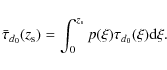
To show more clearly the different behavior in the high-redshift tail of our three choices, we
present their cumulative distributions in the right panel of Fig. 3, namely
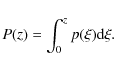
In particular, when
In order to further show that this family of three functions cover
all the reasonable possibilities, we have compared them with the
predictions of one of the semi-analytical models that have been
developed to explain the properties of SMGs (see Swinbank et al. 2008, and references therein). The histogram in the left panel of Fig. 4
shows CH05 data corrected for spectroscopic incompleteness. Note
that the SPZ curve is very consistent with the semi-analytic model
prediction (SWR), although both curves peak at slightly lower redshift
(
![]() )
than the best Gaussian fit of the histogram (SPZC). However, as pointed out in
Swinbank et al. (2008, SW08 hereafter), the CH05 distribution is expected to be uncertain by at least
)
than the best Gaussian fit of the histogram (SPZC). However, as pointed out in
Swinbank et al. (2008, SW08 hereafter), the CH05 distribution is expected to be uncertain by at least
![]() ,
which is the field-to-field variation between the seven sub-fields in
the CH05 sample due to cosmic variance. Therefore, we can consider
SPZ as a good representation of the current observations, despite
the fact that it comes from a histogram that was not corrected for
spectroscopic incompleteness.
,
which is the field-to-field variation between the seven sub-fields in
the CH05 sample due to cosmic variance. Therefore, we can consider
SPZ as a good representation of the current observations, despite
the fact that it comes from a histogram that was not corrected for
spectroscopic incompleteness.
After the computations of the number of arcs were completed, we became aware of the fact that the parameters quoted in CH05 for the best Gaussian fit to their simple evolutionary model (CHM, see Table 1) were incorrect (Swinbank, private communication). As it is shown in the right panel of Fig. 4, the CHM distribution has a higher-z tail as compared to the correct Gaussian fit (CHMC) and the prediction of the semi-analytical model (SWS). Since the true high-z tail of the redshift distribution of SMGs is expected to be in between the cases considered in our calculations (SPZ, PHZ and CHM), and (as it will be discussed in Sect. 5.2) the final effect of the source redshift distribution on the number of arcs is small given the many uncertainties involved, we considered it unnecessary to repeat the calculations for CHMC.
3.3 Source number counts
The final ingredient needed to estimate the number of arcs produced
by SMGs is the observed surface density of this source population, both
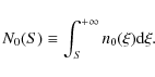
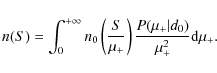
at 1.4 GHz and ![]() m. Let n0(S) be the differential number counts, defined as the surface density of unlensed galaxies per unit flux density
m. Let n0(S) be the differential number counts, defined as the surface density of unlensed galaxies per unit flux density ![]() .
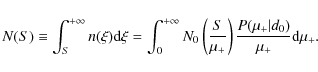
Integrating n0(S) over all fluxes above a given threshold, we obtain the
respective cumulative number counts
.
Integrating n0(S) over all fluxes above a given threshold, we obtain the
respective cumulative number counts
Let
|
(7) |
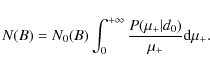
Hence, the magnified cumulative number counts read as
As can be seen in Eq. (8), the lensing magnification bias has a twofold effect. On one side, sources that would be too faint to be detected without the action of lensing are amplified, and hence the respective images are brought above the detection threshold. On the other side, the unit solid angle is stretched by lensing magnification, implying that the number density of sources is decreased. Which one of these two effects wins depends on the local slope of the unmagnified cumulative number counts. In particular, if
Since our main motivation was to provide predictions for the abundance of giant arcs to be detected in surveys carried out with future instruments, we needed to provide the predicted number of arcs as a function of the surface brightness, instead of flux density. The reason is that we are working under the assumption that arcs are resolved structures, and therefore they are observed as extended objects. Under these circumstances, the flux integrated over the resolution element of the instrument (seeing, PSF, pixel or beam) is no longer the total flux of the source (as in the case of unresolved sources), and it may therefore be below the limiting flux although the arc as a whole is not. In other words, arc detectability under these circumstances is not limited by the flux density but rather by the surface brightness.
In order to take this into account, we had to convert the
observed number counts as a function of flux density into number counts
as a function of surface brightness. Assuming that the size of sources
is given by ![]() ,
and that the surface brightness is constant across it, then
,
and that the surface brightness is constant across it, then
![]() .
Note that, since the surface brightness is not affected by lensing, the
magnification bias will manifest itself only through the solid angle
stretching. Therefore, the cumulative magnified number counts
(as a function of surface brightness) can be written as
.
Note that, since the surface brightness is not affected by lensing, the
magnification bias will manifest itself only through the solid angle
stretching. Therefore, the cumulative magnified number counts
(as a function of surface brightness) can be written as
Among other things, this implies that the magnification bias will always decrease the cumulative number counts, irrespective of the shape of the unmagnified ones.
In the following we used the magnification distribution given by Fedeli et al. (2008), which is represented by the superposition of two Gaussians. In particular, we adopted the
![]() function for
d0 = 10, but the result is virtually the same also for the case d0
= 7.5. Note however, that this (conditional) magnification distribution
was computed for a background population of sources that have different
morphologies than SMGs (see Sect. 3.1).
In principle, the bimodality of the magnification distribution is
expected to be preserved because it only depends on the caustic
structure (Li et al. 2005), but it can be affected by the source morphology in two opposite ways. On one hand, since SMGs are smaller than in Fedeli et al. (2008),
we expect large arcs to form closer to
the critical curves, and therefore to have larger magnifications on
average. On the other hand, the fact that SMGs are more elongated will
favor the formation of large arcs in regions of lower
magnification. Given the uncertainties in other parts of the
calculation, we consider that the use of a magnification distribution
derived for optical sources will have a marginal effect on the derived
number of arcs produced by SMGs. For a comprehensive review of the many
effects that could affect the estimation of arc abundances by galaxy
clusters, see the discussion in Fedeli et al. (2008).
function for
d0 = 10, but the result is virtually the same also for the case d0
= 7.5. Note however, that this (conditional) magnification distribution
was computed for a background population of sources that have different
morphologies than SMGs (see Sect. 3.1).
In principle, the bimodality of the magnification distribution is
expected to be preserved because it only depends on the caustic
structure (Li et al. 2005), but it can be affected by the source morphology in two opposite ways. On one hand, since SMGs are smaller than in Fedeli et al. (2008),
we expect large arcs to form closer to
the critical curves, and therefore to have larger magnifications on
average. On the other hand, the fact that SMGs are more elongated will
favor the formation of large arcs in regions of lower
magnification. Given the uncertainties in other parts of the
calculation, we consider that the use of a magnification distribution
derived for optical sources will have a marginal effect on the derived
number of arcs produced by SMGs. For a comprehensive review of the many
effects that could affect the estimation of arc abundances by galaxy
clusters, see the discussion in Fedeli et al. (2008).
3.3.1 Submm number counts
For the latest and most complete estimate of the submm number counts at ![]() m we refer to Knudsen et al. (2008,
hereafter KN08), who carried out a combined analysis of the counts
derived from the Leiden SCUBA Lens Survey (LSLS) and the
SHADES survey. With an area of 720 arcmin2, the
SHADES survey is the largest blank-field submm survey completed to
date, and therefore the least affected by cosmic variance.
It provides the best constraints for the
submm number counts in the flux density range 2-15 mJy (Coppin et al. 2006). On the other hand, the LSLS survey targeted 12 galaxy cluster fields which cover a total area of 71.5 arcmin2
in the image plane. It provides the deepest constraints at the
faint end of the submm counts (0.11 mJy, after correcting for the
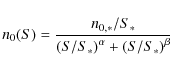
lensing magnification). In their analysis, KN08 used two functions
to characterize the combined differential number counts from both
surveys: a double power-law,
m we refer to Knudsen et al. (2008,
hereafter KN08), who carried out a combined analysis of the counts
derived from the Leiden SCUBA Lens Survey (LSLS) and the
SHADES survey. With an area of 720 arcmin2, the
SHADES survey is the largest blank-field submm survey completed to
date, and therefore the least affected by cosmic variance.
It provides the best constraints for the
submm number counts in the flux density range 2-15 mJy (Coppin et al. 2006). On the other hand, the LSLS survey targeted 12 galaxy cluster fields which cover a total area of 71.5 arcmin2
in the image plane. It provides the deepest constraints at the
faint end of the submm counts (0.11 mJy, after correcting for the
lensing magnification). In their analysis, KN08 used two functions
to characterize the combined differential number counts from both
surveys: a double power-law,
and a Schechter function (Schechter 1976),
![\begin{figure}
\par\includegraphics[width=8.5cm,clip]{Figures/2884f5}
\end{figure}](/articles/aa/full_html/2009/46/aa12884-09/img115.png)
|
Figure 5: Comparison between
observed and predicted cumulative number
counts. The red and black solid curves corresponds to the best-fit
double power-law (DB) and the best-fit Schechter function (SB) derived
by Knudsen et al. (2008) for the combined |
| Open with DEXTER | |
Moreover, when fitting the observed cumulative number counts, they added the supplementary constraint that the integrated light well below 0.1 mJy should not be higher than the extragalactic background light (Fixsen et al. 1998; Puget et al. 1996). The resulting best-fit parameters are summarized in Table 2.
Figure 5
shows the (unmagnified) cumulative number counts derived from the best
fit Schechter function (black solid line) and the best fit double power
law function (red
solid line) presented in KN08 using Eq. (6).
Note that, whereas both curves behave almost identically at the bright
flux end, their predictions for the low flux number counts differ by a
factor of ![]() at 0.1 mJy. Since the low flux tail of the submm counts
dominates the number of SMGs that could potentially be lensed, we
computed predictions for arcs produced by SMGs at
at 0.1 mJy. Since the low flux tail of the submm counts
dominates the number of SMGs that could potentially be lensed, we
computed predictions for arcs produced by SMGs at ![]() m for the two following cases: (i) the shallowest Schechter function consistent
with the combined LSLS and SHADES data (also shown in Fig. 5)
and (ii) the best fit double power law function, hereafter
refered to as SM and DB, respectively. The first one provides the
minimum expected number of arcs consistent with observations, whereas
the second one gives the number of arcs predicted by the best fit to
the data (see Table 2).
m for the two following cases: (i) the shallowest Schechter function consistent
with the combined LSLS and SHADES data (also shown in Fig. 5)
and (ii) the best fit double power law function, hereafter
refered to as SM and DB, respectively. The first one provides the
minimum expected number of arcs consistent with observations, whereas
the second one gives the number of arcs predicted by the best fit to
the data (see Table 2).
Table 2:
Parameters for the ![]() m differential number counts.
m differential number counts.
![\begin{figure}
\par\includegraphics[width=8.5cm,clip]{Figures/2884f6a}\hspace*{1...
...hspace*{1cm}
\includegraphics[width=8.5cm,clip]{Figures/2884f6d} %
\end{figure}](/articles/aa/full_html/2009/46/aa12884-09/img127.png)
|
Figure 6:
The cumulative number counts of SMGs at |
| Open with DEXTER | |
The cumulative number counts derived for these two cases as a function of flux density are shown in the top left panel of Fig. 6, including the corresponding counts corrected for magnification bias using Eq. (8). In the same figure, the top right panel shows the cumulative number counts as function of surface brightness. The corresponding counts corrected for magnification bias (which will be used to compute the number of arcs) were derived using Eq. (9).
3.3.2 Radio number counts
Figure 5
also shows the cumulative submm number counts predicted by the
SW08 model (blue solid line) compared with the results from
different ![]() m
SCUBA surveys. Note that, although the model tends to over-predict
the counts at faint fluxes compared with the best fits provided by KN08
(red and black solid lines), it is consistent with the observational
errors. The cyan solid line indicates the predicted counts for SMGs
with radio counterparts assuming
m
SCUBA surveys. Note that, although the model tends to over-predict
the counts at faint fluxes compared with the best fits provided by KN08
(red and black solid lines), it is consistent with the observational
errors. The cyan solid line indicates the predicted counts for SMGs
with radio counterparts assuming
![]() Jy. The fact that its shape is different from the shape of the blue solid
curve is because current observations only detect radio emission from
Jy. The fact that its shape is different from the shape of the blue solid
curve is because current observations only detect radio emission from
![]() of the observed SMGs. However, if we allow the sensitivity threshold to go down to the
of the observed SMGs. However, if we allow the sensitivity threshold to go down to the ![]() Jy level expected for e-MERLIN, the SW08 model indicates that it would be possible to detect all the radio counterparts of SMGs with
Jy level expected for e-MERLIN, the SW08 model indicates that it would be possible to detect all the radio counterparts of SMGs with
![]() mJy (cyan dashed line).
mJy (cyan dashed line).
Since SMGs seem to follow the FIR/radio correlation (e.g. Kovács et al. 2006), the
![]() number counts of SMGs (which we need to predict the number of radio arcs) could be derived by scaling the
number counts of SMGs (which we need to predict the number of radio arcs) could be derived by scaling the ![]() m number counts introduced in the previous section (DB and SM). As shown in Fig. 7 of CH05, the ratio between the
m number counts introduced in the previous section (DB and SM). As shown in Fig. 7 of CH05, the ratio between the ![]() m
flux density and the 1.4 GHz flux density shows a broad scatter
(up to one order of magnitude), which is probably a consequence of
the strong influence of the dust temperature on the SEDs of SMGs.
However, most of the points in this figure are located between
redshift 2 and 3, and have an average
m
flux density and the 1.4 GHz flux density shows a broad scatter
(up to one order of magnitude), which is probably a consequence of
the strong influence of the dust temperature on the SEDs of SMGs.
However, most of the points in this figure are located between
redshift 2 and 3, and have an average
![]() ratio between 50 and 100. Therefore, we decided to use these
two scaling factors to derive first order upper
and lower limits of the radio number counts of SMGs. The resultant
cumulative radio number counts are shown in the lower panels of
Fig. 6.
Note that the values of 50 and 100 chosen for the submm/radio
flux density ratio are meant to be indicative, since there are still
many sources that display a ratio below 50 or above 100. The
reader interested in results given by different values of this ratio
can scale the curves appropriately in the upper panels of Fig. 6. Also, exact numerical values can be made available by the authors upon request.
ratio between 50 and 100. Therefore, we decided to use these
two scaling factors to derive first order upper
and lower limits of the radio number counts of SMGs. The resultant
cumulative radio number counts are shown in the lower panels of
Fig. 6.
Note that the values of 50 and 100 chosen for the submm/radio
flux density ratio are meant to be indicative, since there are still
many sources that display a ratio below 50 or above 100. The
reader interested in results given by different values of this ratio
can scale the curves appropriately in the upper panels of Fig. 6. Also, exact numerical values can be made available by the authors upon request.
4 Strong lensing optical depth
To compute the total optical depth for lensed SMGs, we constructed a synthetic cluster population composed of q = 1000 cluster-sized dark-matter halos with masses uniformly distributed in the interval [1014, 2.5 ![]() 1015]
1015]
![]() at z=0.
Note that it is not necessary to extract these masses according to the
cluster mass function, since this is already taken into account in
Eq. (1) by weighting the cross sections with the function n(M,z). The structure of each cluster is modeled using the NFW density profile (Navarro et al. 1995,1997,1996),
which constitutes a good representation of average dark-matter halos
over a wide range of masses, redshifts and cosmologies in numerical n-body simulations
(Dolag et al. 2004). Several studies of strong lensing and X-ray luminous clusters also show that these are well fitted by an NFW profile (Schmidt & Allen 2007; Oguri et al. 2009). This profile also has the advantage that its lensing properties can be described analytically (Bartelmann 1996).
at z=0.
Note that it is not necessary to extract these masses according to the
cluster mass function, since this is already taken into account in
Eq. (1) by weighting the cross sections with the function n(M,z). The structure of each cluster is modeled using the NFW density profile (Navarro et al. 1995,1997,1996),
which constitutes a good representation of average dark-matter halos
over a wide range of masses, redshifts and cosmologies in numerical n-body simulations
(Dolag et al. 2004). Several studies of strong lensing and X-ray luminous clusters also show that these are well fitted by an NFW profile (Schmidt & Allen 2007; Oguri et al. 2009). This profile also has the advantage that its lensing properties can be described analytically (Bartelmann 1996).
To account for the asymmetries of real galaxy clusters, the halos are
assumed to have elliptically distorted lensing potentials. However,
instead of considering a single ellipticity value to describe all the
synthetic cluster lenses, we derived an ellipticity distribution from a
set of numerical clusters extracted from the MareNostrum simulation (Gottlöber & Yepes 2007).
The strong lensing analysis required to generate this ellipticity
distribution was taken from Fedeli et al. (2009,
in preparation), as described in Sect. 3.1.
For each simulated cluster, the lensing analysis along three orthogonal
projections was performed, computing the cross sections for arcs with
![]() and sources with
and sources with
![]() .
For each of these projections, we found the ellipticity e of the NFW lens whose cross section is closest to the cross section of the numerical
cluster, i.e., we found the ellipticity that minimizes the quantity
.
For each of these projections, we found the ellipticity e of the NFW lens whose cross section is closest to the cross section of the numerical
cluster, i.e., we found the ellipticity that minimizes the quantity
where
![\begin{figure}
\par\includegraphics[width=8.5cm,clip]{Figures/2884f7}
\end{figure}](/articles/aa/full_html/2009/46/aa12884-09/img136.png)
|
Figure 7: The distribution of NFW lens ellipticities fitting the cross sections of a sample of numerical clusters. The red dashed line represents the best fit log-normal distribution, whose median and dispersion are labeled in the top-right corner of the plot. |
| Open with DEXTER | |
Figure 7 shows the distribution of the ellipticities that minimize the quantity r(e) in Eq. (12)
for all clusters in our numerical analysis. The dashed red line is
derived by fitting the distribution with a log-normal function of
the kind
![\begin{displaymath}%
p(e){\rm d}e = \frac{1}{\sqrt{2\pi}\sigma_{\rm e}} \exp\lef...
... - \ln(e_0)\right]^2}{2\sigma_{\rm e}^2}\right] {\rm d}\ln(e),
\end{displaymath}](/articles/aa/full_html/2009/46/aa12884-09/img137.png)
where the best-fit parameters are e0 = 0.31 and
Elliptical NFW profiles are a good representation of realistic
cluster lenses only when the clusters do not undergo major merger
events (Meneghetti et al. 2003). Since the merger activity of galaxy clusters is known to have a significant effect on the statistics of giant arcs (Torri et al. 2004; Fedeli et al. 2006),
it has to be taken into account in the construction of the synthetic
cluster population. For this reason, we used the excursion set formalism![]() developed by Lacey & Cole (1993) (see also Somerville & Kolatt 1999; Bond et al. 1991) to construct a backward merger tree for each model cluster at z = 0, assuming that each merger is binary (see discussion in Fedeli & Bartelmann 2007).
When a merger happens, the event is modeled assuming that the two
merging halos (also described as elliptical NFW density profiles)
approach each other at a constant
speed. The duration of the merger is set by the dynamical timescales of
the two halos (see Fedeli & Bartelmann 2007; and Fedeli et al. 2008, for a detailed description of the modeling procedure).
developed by Lacey & Cole (1993) (see also Somerville & Kolatt 1999; Bond et al. 1991) to construct a backward merger tree for each model cluster at z = 0, assuming that each merger is binary (see discussion in Fedeli & Bartelmann 2007).
When a merger happens, the event is modeled assuming that the two
merging halos (also described as elliptical NFW density profiles)
approach each other at a constant
speed. The duration of the merger is set by the dynamical timescales of
the two halos (see Fedeli & Bartelmann 2007; and Fedeli et al. 2008, for a detailed description of the modeling procedure).
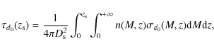
With the synthetic cluster population constructed in this way, the
total average optical depth was derived by computing individual cross
sections with the semi-analytic algorithm developed by Fedeli et al. (2006),
especially designed to estimate the strong lensing cross sections of
individual lenses in a fast and reliable way. The optical depth for a
discrete set of lenses can be recast as
![\begin{displaymath}%
\tau_{d_0}(z_{\rm s}) = \frac{1}{4\pi D_{\rm s}^2} \int_0^{...
...0,i}(z) \int_{M_i}^{M_{i+1}} n(M,z) {\rm d}M \right] {\rm d}z,
\end{displaymath}](/articles/aa/full_html/2009/46/aa12884-09/img139.png)
where the masses Mi (
![\begin{displaymath}%
\bar{\sigma}_{d_0,i}(z) \equiv \frac{1}{2} \left[ \sigma_{d_0}(M_i,z) + \sigma_{d_0}(M_{i+1},z) \right].
\end{displaymath}](/articles/aa/full_html/2009/46/aa12884-09/img142.png)
|
(15) |
This effectively means that, for all the clusters with mass between Mi and Mi+1, we assume the average cross section of the model dark-matter halos with masses Mi and Mi+1. The algorithm of Fedeli et al. (2006) for computing strong lensing cross sections consists of first assuming sources as point-like circles, and then introducing the effect of source ellipticity according to Keeton (2001). The source finite size is taken into account by convolving the local lensing properties over the typical source size.
![\begin{figure}
\par\includegraphics[width=8.5cm,clip]{Figures/2884f8a}\hspace*{0.7cm}
\includegraphics[width=8.5cm,clip]{Figures/2884f8b}
\end{figure}](/articles/aa/full_html/2009/46/aa12884-09/img143.png)
|
Figure 8:
Left panel: differential redshift distributions of SMGs
producing large gravitational arcs, corresponding to the cumulative
distributions reported in the right panel. Right panel: the cumulative redshift distributions of SMGs producing radio
arcs with
|
| Open with DEXTER | |
The total average optical depth is calculated by integrating Eq. (14) over the source redshift distribution. Effectively, the
![]() weighting is avoided since we assigned individual source redshifts (randomly extracted from the distribution
weighting is avoided since we assigned individual source redshifts (randomly extracted from the distribution
![]() )
at each of the q halos
in the cluster sample and evolved their merger trees back in time until
the respective source redshift. Given the large number of synthetic
dark-matter halos used, this approach allows one to omit
)
at each of the q halos
in the cluster sample and evolved their merger trees back in time until
the respective source redshift. Given the large number of synthetic
dark-matter halos used, this approach allows one to omit
![]() in Eq. (2) when the redshift integral is discretized.
in Eq. (2) when the redshift integral is discretized.
Despite the fact that the ellipticity distribution used to model the synthetic cluster population was derived for
![]() ,
the best fit parameters of Eq. (13) can be used to compute the cross sections for arcs also with d0
= 10 without compromising the results. The reason is that, although
there might be a mild dependence of the distribution of lensing
ellipticities on d0, it is the overall caustic structure that defines the abundance of arcs above a certain d0,
regardless of its precise value. In fact, the criterion used to
determine the ellipticity distribution is based on the similarity
between the cross sections of the NFW lens and
the numerical lens, which is an indirect way of comparing the overall
caustic structures produced by both kinds of lenses. To verify
this argument, the ellipticity distribution was re-computed using a
criterion that is directly related to the caustic structure, that is,
by defining the best fitting ellipticity as the one that minimizes the
modified Hausdorff distance
,
the best fit parameters of Eq. (13) can be used to compute the cross sections for arcs also with d0
= 10 without compromising the results. The reason is that, although
there might be a mild dependence of the distribution of lensing
ellipticities on d0, it is the overall caustic structure that defines the abundance of arcs above a certain d0,
regardless of its precise value. In fact, the criterion used to
determine the ellipticity distribution is based on the similarity
between the cross sections of the NFW lens and
the numerical lens, which is an indirect way of comparing the overall
caustic structures produced by both kinds of lenses. To verify
this argument, the ellipticity distribution was re-computed using a
criterion that is directly related to the caustic structure, that is,
by defining the best fitting ellipticity as the one that minimizes the
modified Hausdorff distance![]() between the critical lines of the numerical and NFW lenses. The
ellipticity distribution obtained in this way is very similar to the
one depicted in Fig. 7 (
e0 = 0.30,
between the critical lines of the numerical and NFW lenses. The
ellipticity distribution obtained in this way is very similar to the
one depicted in Fig. 7 (
e0 = 0.30,
![]() ).
).
The median of the ellipticity distribution derived in this work using the lensing cross section (
e0 = 0.31, see Fig. 7) is fully consistent with the one obtained by Meneghetti et al. (2003) comparing the deflection angle maps (
![]() ,
using lenses placed at
,
using lenses placed at
![]() and a source population at
and a source population at
![]() ).
Even though these two criteria are arguably tightly related, the former
is a quantity that is more directly related to observables than the
latter, hence it is reassuring that they give comparable results. In
addition, this result extends the previous one by quantifying the
scatter around the median ellipticity and dealing with lenses that are
distributed in redshift.
).
Even though these two criteria are arguably tightly related, the former
is a quantity that is more directly related to observables than the
latter, hence it is reassuring that they give comparable results. In
addition, this result extends the previous one by quantifying the
scatter around the median ellipticity and dealing with lenses that are
distributed in redshift.
5 Results
5.1 Arc redshift distribution
The redshift distribution of arcs with ![]() (arc redshift
distribution hereafter) is expected to provide information about the
redshift distribution of the background source population that is
being lensed. However, it will also be distorted by the fact that
the abundance of massive and compact galaxy clusters evolves with
redshift, and that the lensing efficiency depends on the relative
distances of sources and lens with respect to the observer.
(arc redshift
distribution hereafter) is expected to provide information about the
redshift distribution of the background source population that is
being lensed. However, it will also be distorted by the fact that
the abundance of massive and compact galaxy clusters evolves with
redshift, and that the lensing efficiency depends on the relative
distances of sources and lens with respect to the observer.
To assess the potential of this approach to gather information
about the intrinsic redshift distribution of SMGs, we derived the arc
redshift distribution associated with each of the
three source redshift distributions used as inputs in our calculations
(see Fig. 3). This was done by computing, for each input distribution, the average optical depth
![]() for several different values of
for several different values of ![]() .
That is, we excluded in the computation of the average optical depth
those model clusters (and their respective chain of progenitors)
whose associated source redshifts were
.
That is, we excluded in the computation of the average optical depth
those model clusters (and their respective chain of progenitors)
whose associated source redshifts were
![]() .
The resultant cumulative arc redshift distributions, obtained after normalizing the optical depth for each
.
The resultant cumulative arc redshift distributions, obtained after normalizing the optical depth for each ![]() to the total average optical depth
to the total average optical depth
![]() ,
are shown in the right panel of Fig. 8. The lines correspond to the best fit for each distribution provided by the simple function
,
are shown in the right panel of Fig. 8. The lines correspond to the best fit for each distribution provided by the simple function
where
Table 3: Parameters of the arc redshift distributions shown in Fig. 8.
Once more, these arc redshift distributions have been shown for arcs with length-to-width ratio larger than d0 = 10 only. As we verified, since the relative contribution of individual model clusters to the total average optical depth is the same for both d0 = 7.5 and d0 = 10, the resulting arc redshift distribution also does not change significantly between the two choices.
A comparison between Figs. 8 and 3
shows that, as expected, the arc redshift distributions reflect the
general properties of the source redshift distributions used as input,
but
there are also some noteworthy differences between them. For instance,
the arc redshift distribution associated with CHM tends to zero at very
low redshift, unlike in the case of the original CHM distribution.
The reason is that low redshift sources do not produce many arcs,
because (i) they have very few potential lenses at their disposal;
and (ii) the lensing efficiency of those lenses is very low due to
geometric suppression. This results in a lack of low redshift arcs in
the distribution, which shifts its peak to higher redshifts compared
with the CHM peak (from
![]() to
to
![]() ). Similarly, the peak of the arc redshift distribution corresponding to SPZ is shifted from
). Similarly, the peak of the arc redshift distribution corresponding to SPZ is shifted from
![]() to
to
![]() .
.
On the other hand, the arc redshift distribution corresponding to PHZ
is not significantly shifted but visibly narrowed. As in the
previous cases, low-redshift sources are removed from the distribution
because they cannot produce arcs, but the distribution could not shift
at higher redshift because the input source redshift distribution is
immediately truncated at
![]() .
In other words, there is too little room between the drop due to
lensing efficiency and the one due to the cutoff of the input
distribution to allow a significant shift in its peak, and the only
possible consequence for the distribution is to shrink and increase the
peak height in order to preserve the normalization.
.
In other words, there is too little room between the drop due to
lensing efficiency and the one due to the cutoff of the input
distribution to allow a significant shift in its peak, and the only
possible consequence for the distribution is to shrink and increase the
peak height in order to preserve the normalization.
In general, it is apparent that the differences between different source redshift distributions are somewhat enhanced when it comes to the arc redshift distribution. Therefore, assuming that redshift information is available for arcs, this approach can in principle be used to obtain some information about the general characteristics of the source redshift distribution, although it will probably not allow one to distinguish between redshift distributions that are very similar.
5.2 Number of radio and submm arcs
In this section we present and discuss the main results of this work: the predicted number of arcs produced by SMGs at radio and submm wavelengths. To that end, we computed the total average optical depth for each of the three source redshift distributions presented in Sect. 3.2 (PHZ, SPZ and CHM), and for arcs with length-to-width ratio higher than both d0 = 7.5 and d0 = 10. These quantities were then multiplied by the magnified cumulative source number counts presented in Sect. 3.3 (SM and DB), to obtain the arc number counts as function of surface brightness. The results, extrapolated to the whole sky, are shown in Fig. 9. A detailed list with the predicted number of submm and radio arcs for different sensitivities is presented in Tables 4 and 6, respectively.
Note that the arc number counts given by the source redshift
distributions SPZ and PHZ are almost indistinguishable on the
scale of Fig. 9, irrespective of the length-to-width
threshold d0 adopted. As expected, SPZ produces more large arcs than PHZ because it peaks at higher redshift, but only by a factor of ![]() .
The redshift distribution CHM, on the other hand, produces more large arcs than the other two by a factor of
.
The redshift distribution CHM, on the other hand, produces more large arcs than the other two by a factor of ![]() .
Since, as mentioned in Sect. 3.2,
the distributions CHM and PHZ can be considered as upper and lower
limits to the true redshift distribution respectively, we can conclude
that the uncertainty introduced by the redshift distribution in the
predicted number of arcs is less than a factor of two.
.
Since, as mentioned in Sect. 3.2,
the distributions CHM and PHZ can be considered as upper and lower
limits to the true redshift distribution respectively, we can conclude
that the uncertainty introduced by the redshift distribution in the
predicted number of arcs is less than a factor of two.
![\begin{figure}
\par\includegraphics[width=8.5cm,clip]{Figures/2884f9a}\hspace*{0...
...
\includegraphics[width=8.5cm,clip]{Figures/2884f9d}
\vspace*{3mm}
\end{figure}](/articles/aa/full_html/2009/46/aa12884-09/img158.png)
|
Figure 9:
The total number of arcs with
|
| Open with DEXTER | |
In terms of the length-to-width threshold, the number of arcs predicted for d0 = 7.5 is larger than for d0 = 10 (as was also expected). However, the ratio between the number of arcs with
![]() and
and
![]() is not exactly equal to the ratio in the respective optical depths,
since the magnification distributions for the two kinds of arcs are
also different (see the discussion in Fedeli et al. 2008).
is not exactly equal to the ratio in the respective optical depths,
since the magnification distributions for the two kinds of arcs are
also different (see the discussion in Fedeli et al. 2008).
Finally, when it comes to comparing the results from the two adopted
source number counts (DB and SM), we see that the difference
in the predicted number of arcs is negligible for submm surface
brightness limits greater than 5 mJy arcsec-2. However, at
![]() mJy arcsec-2,
the function DB predicts 2 times more arcs than SM, and
the difference becomes a factor of 5 for 0.1 mJy arcsec-2. In the radio domain, the difference between DB and SM is negligible for
mJy arcsec-2,
the function DB predicts 2 times more arcs than SM, and
the difference becomes a factor of 5 for 0.1 mJy arcsec-2. In the radio domain, the difference between DB and SM is negligible for
![]() Jy arcsec-2, a factor
Jy arcsec-2, a factor ![]() for
for ![]() Jy arcsec-2, a factor
Jy arcsec-2, a factor ![]() for
for ![]() Jy arcsec-2 and a factor
Jy arcsec-2 and a factor ![]() for
for ![]() Jy arcsec-2.
Therefore, the uncertainty in the predicted number of arcs is clearly
dominated by the uncertainty of the source number counts at the faint
surface brightness end.
Jy arcsec-2.
Therefore, the uncertainty in the predicted number of arcs is clearly
dominated by the uncertainty of the source number counts at the faint
surface brightness end.
Considering an all-sky submm survey with enough resolution to resolve individual arcs with
![]() (
(
![]() ), and a sensitivity of
), and a sensitivity of
![]() mJy arcsec-2, our calculations predict between
mJy arcsec-2, our calculations predict between ![]() (PHZ SM) and
(PHZ SM) and ![]() (SPZ DB) arcs with a signal-to-noise ratio (SNR) larger than 5. In the case of
(SPZ DB) arcs with a signal-to-noise ratio (SNR) larger than 5. In the case of
![]() ,
the expected number of arcs would be between 200 and 250. If the sensitivity is reduced to 0.1 mJy arcsec-2, these predictions can vary between
,
the expected number of arcs would be between 200 and 250. If the sensitivity is reduced to 0.1 mJy arcsec-2, these predictions can vary between
![]() and
and
![]() for d0=7.5, and between 1400 and 3600 for d0=10.
for d0=7.5, and between 1400 and 3600 for d0=10.
In a similar way, an all sky radio survey with a sensitivity of
![]() mJy arcsec-2 would detect between 8 and 50 arcs for d0=7.5 (between none and 25 for d0=10) at SNR
mJy arcsec-2 would detect between 8 and 50 arcs for d0=7.5 (between none and 25 for d0=10) at SNR ![]() 5, with the main uncertainty given by the
5, with the main uncertainty given by the
![]() ratio
used to obtain the radio number counts by scaling the observed submm
counts. If the limiting radio surface brightness is reduced to
ratio
used to obtain the radio number counts by scaling the observed submm
counts. If the limiting radio surface brightness is reduced to
![]() Jy arcsec-2, the predicted number of arcs could be increased to
Jy arcsec-2, the predicted number of arcs could be increased to
![]() for d0=7.5 (200-600 for d0=10). In order to have excellent statistics with a few thousand giant arcs with SNR
for d0=7.5 (200-600 for d0=10). In order to have excellent statistics with a few thousand giant arcs with SNR ![]() 5, it would be necessary to go as deep as
5, it would be necessary to go as deep as
![]() Jy arcsec-2.
The largest number of arcs is given by the CHM source redshift
distribution, which is about a factor of 2 larger than the number
of arcs predicted by SPZ and PHZ.
Jy arcsec-2.
The largest number of arcs is given by the CHM source redshift
distribution, which is about a factor of 2 larger than the number
of arcs predicted by SPZ and PHZ.
It is plausible that future radio and submillimeter surveys of
galaxy clusters would focus on the most massive objects, since the
center of attention of many multiwavelength studies is on X-ray bright
clusters. To roughly evaluate the effect of this kind of
selection, we re-computed the optical depths by including only those
clusters in our synthetic population with mass ![]()
![]()
![]() .
The resulting arc number counts are presented in Fig. 10, where we used the same scale and line types as in Fig. 9
to ease comparison. The corresponding numbers of submm and radio arcs
predicted for different sensitivities are listed in Tables 5 and 7,
respectively. The most interesting feature about these new plots is
that the relative difference in the arc number counts produced by the
CHM distribution on the one hand, and PHZ and SPZ on the other, is
significantly reduced. This is due to the fact that massive clusters
are found mainly at low redshift, hence lower-mass higher-redshift
lenses, that are accessible only to the CHM distribution, become
unimportant.
.
The resulting arc number counts are presented in Fig. 10, where we used the same scale and line types as in Fig. 9
to ease comparison. The corresponding numbers of submm and radio arcs
predicted for different sensitivities are listed in Tables 5 and 7,
respectively. The most interesting feature about these new plots is
that the relative difference in the arc number counts produced by the
CHM distribution on the one hand, and PHZ and SPZ on the other, is
significantly reduced. This is due to the fact that massive clusters
are found mainly at low redshift, hence lower-mass higher-redshift
lenses, that are accessible only to the CHM distribution, become
unimportant.
Table 4:
Predicted number of submm (![]() m) arcs produced by SMGs
for an all-sky survey, using all the synthetic cluster population to compute the optical depths (see Fig. 9).
m) arcs produced by SMGs
for an all-sky survey, using all the synthetic cluster population to compute the optical depths (see Fig. 9).
Table 5:
Predicted number of submm (![]() m) arcs produced by SMGs
for an all-sky survey, using only clusters with
m) arcs produced by SMGs
for an all-sky survey, using only clusters with ![]()
![]()
![]() to compute the optical depths (see Fig. 10).
to compute the optical depths (see Fig. 10).
The order-of-magnitude reduction in the abundance of giant arcs when focusing only on clusters with mass ![]()
![]()
![]() is
in agreement with the fact that the bulk of the lensing signal actually
comes from low-mass clusters, since the optical depth is obviously
dominated by the lowest mass objects that are capable of producing a
non-vanishing cross sections (see Eq. (1)). Note also that, unlike the previous case, PHZ produces slightly more arcs
than SPZ. This is due to the fact that we are including in the calculations only low-z clusters, and PHZ actually has more sources with, e.g.,
is
in agreement with the fact that the bulk of the lensing signal actually
comes from low-mass clusters, since the optical depth is obviously
dominated by the lowest mass objects that are capable of producing a
non-vanishing cross sections (see Eq. (1)). Note also that, unlike the previous case, PHZ produces slightly more arcs
than SPZ. This is due to the fact that we are including in the calculations only low-z clusters, and PHZ actually has more sources with, e.g.,
![]() than SPZ (see Fig. 3).
than SPZ (see Fig. 3).
![\begin{figure}
\par\includegraphics[width=8.5cm,clip]{Figures/2884f10a}\hspace*{...
...space*{0.8cm}
\includegraphics[width=8.5cm,clip]{Figures/2884f10d}
\end{figure}](/articles/aa/full_html/2009/46/aa12884-09/img183.png)
|
Figure 10:
The total number of arcs with
|
| Open with DEXTER | |
Considering again an all-sky submm survey with enough resolution to resolve individual arcs with
d0 = 7.5 and sensitivity of
![]() mJy arcsec-2, we predict
mJy arcsec-2, we predict ![]() arcs with
arcs with
![]() (8 if d0=10). This number can increase to 100-250 (40-90) if
(8 if d0=10). This number can increase to 100-250 (40-90) if
![]() mJy arcsec-2. In the case of a radio survey, it would be necessary to push the limiting flux density down to
mJy arcsec-2. In the case of a radio survey, it would be necessary to push the limiting flux density down to
![]() Jy arcsec-2 to detect few hundred arcs (between 40-200 if d0=10).
Jy arcsec-2 to detect few hundred arcs (between 40-200 if d0=10).
6 Comparison with previous work
The probability of strong gravitational lensing due to background
sources at radio and submm wavelengths has been a poorly studied issue
in the past years. In addition, the few works available in the
literature usually involve cosmological models, deflector mass ranges,
and modeling approaches for the source and lens populations that are
different from the ones used in the present work, making the comparison
between them difficult and often not possible. With this note of
caution, we tried however to make some of these tentative comparisons
in the following. This required us to repeat the calculations in the
last section using the number counts as a function of flux density
instead of surface brightness. The results are shown in Fig. 11 only for arcs with
![]() .
.
6.1 Submm wavelengths
Given the poor resolution of current submm instruments, observational studies of submm arcs have not been possible so far, with only one submm arc candidate reported until now. This arc is supposed to be the brightest region of the extended submm source SMM J 04542-0301, located in the core of the cluster MS 0451.6-0305 (Berciano Alba et al. 2007; Borys et al. 2004; Berciano Alba et al. 2009, in press). However, higher resolution submm observations are required in order to confirm this hypothesis, and meaningful estimates of the length and width of this source, unfortunately, cannot yet be done. On the theoretical side, gravitational lensing of SMGs due to galaxy clusters was first studied by Blain (1997), using a circularly symmetric model of the cluster A2218 and the submm counts predicted by different galaxy evolution models. More recent studies (Cooray 1999; Paciga et al. 2009) also have been focused on predicting the number of submm lensed sources, but predictions for the abundance of submm arcs have never been attempted before.
For instance, in the work of Paciga et al. (2009), the authors employ the strong lensing analysis of the Millennium Simulation performed by Hilbert et al. (2007) (see also Hilbert et al. 2008) in order to compute (i) the average magnification of SMGs as a function of flux density; and (ii) the contribution to the differential number counts given by sources with different redshifts and magnifications. Hence, their results cannot be compared with ours in a straightforward way.
The only work with which we could try a tentative comparison is the one by Cooray (1999,
CO99 hereafter), where the author provides number counts of (among
others) gravitationally lensed submm sources as a function of their
magnification. The clusters were modeled as Singular Isothermal Sphere
(SIS henceforth) density profiles, which means that the image
magnification equals its length-to-width ratio, as long as sources
are circular and point-like. Since the sources that we are using are
not circular, nor point-like, the following comparison should be taken
with caution. The background submm sources were described by means of
the redshift and number distributions observed in the Hubble Deep Field
(HDF). Using a ![]() CDM cosmology, and considering cluster lenses with
CDM cosmology, and considering cluster lenses with ![]()
![]()
![]() ,
CO99 predicted
,
CO99 predicted ![]() submm sources in the whole sky with lensing magnification larger than 10 and
submm sources in the whole sky with lensing magnification larger than 10 and
![]() mJy.
mJy.
On the other hand, our results indicate that, if no mass selection is applied and for
![]() mJy, we should find a few thousand arcs with
mJy, we should find a few thousand arcs with
![]() in the whole sky. Restricting the cluster mass range to
in the whole sky. Restricting the cluster mass range to ![]()
![]()
![]() reduces the number of arcs to
reduces the number of arcs to ![]() at most. Matching the mass range of CO99 would only reduce the number
of predicted arcs even further, hence being discrepant with
CO99 predictions. Assuming that the source population we are
considering is the same, we ascribe at least part of this disagreement
to the fact that CO99 considers a very high normalization of the power
spectrum (
at most. Matching the mass range of CO99 would only reduce the number
of predicted arcs even further, hence being discrepant with
CO99 predictions. Assuming that the source population we are
considering is the same, we ascribe at least part of this disagreement
to the fact that CO99 considers a very high normalization of the power
spectrum (
![]() ), which was
based on old studies of the cluster temperature function (Viana & Liddle 1996). As shown in Fedeli et al. (2008), this results in greater strong lensing optical depth, and therefore to an over-prediction of
the number of lensed images.
), which was
based on old studies of the cluster temperature function (Viana & Liddle 1996). As shown in Fedeli et al. (2008), this results in greater strong lensing optical depth, and therefore to an over-prediction of
the number of lensed images.
6.2 Radio wavelengths
Table 6: Predicted number of radio (1.4 GHz) arcs produced by SMGs for an all-sky survey, using all the synthetic cluster population to compute the optical depths (see Fig. 9).
Table 7:
Predicted number of radio (1.4 GHz) arcs produced by SMGs for
an all-sky survey, using only clusters with ![]()
![]()
![]() to compute the optical depths (see Fig. 10).
to compute the optical depths (see Fig. 10).
The first observational search for radio arcs in galaxy clusters dates back to Bagchi & Kapahi (1995), where the authors considered a cluster sample of 46 objects with ![]() observed, among others, at a
wavelength of 20 cm with a sensitivity of
observed, among others, at a
wavelength of 20 cm with a sensitivity of ![]() mJy.
They claimed a systematic tangential alignment of radio images with
respect to the cluster centers, and concluded that these are arclets or
even giant arcs produced by background flat-spectrum radio sources.
While their resolution was too poor to reliably measure arc
morphological properties, these findings were subsequently questioned
by Andernach et al. (1998), who performed a similar analysis on the Abell et al. (1989)
cluster sample (ACO henceforth) with sources taken from the FIRST
(Faint Images of the Radio Sky at Twenty-centimeters) catalogue (White et al. 1997),
finding no evidence for a preferential alignment of radio images in the
core of massive galaxy clusters. They also report a rough estimate of
the abundance of strong lensing events that should be seen in ACO
clusters, finding that for a statistically significant detection, the
limiting flux density should be lowered to
mJy.
They claimed a systematic tangential alignment of radio images with
respect to the cluster centers, and concluded that these are arclets or
even giant arcs produced by background flat-spectrum radio sources.
While their resolution was too poor to reliably measure arc
morphological properties, these findings were subsequently questioned
by Andernach et al. (1998), who performed a similar analysis on the Abell et al. (1989)
cluster sample (ACO henceforth) with sources taken from the FIRST
(Faint Images of the Radio Sky at Twenty-centimeters) catalogue (White et al. 1997),
finding no evidence for a preferential alignment of radio images in the
core of massive galaxy clusters. They also report a rough estimate of
the abundance of strong lensing events that should be seen in ACO
clusters, finding that for a statistically significant detection, the
limiting flux density should be lowered to ![]() mJy, in agreement with previous, more detailed estimates (Wu & Hammer 1993). More recently, Phillips et al. (2001)
searched for strong lensing events with large angular separations in
the FIRST catalog, but none of their candidates turned out to be a real
gravitational lens.
mJy, in agreement with previous, more detailed estimates (Wu & Hammer 1993). More recently, Phillips et al. (2001)
searched for strong lensing events with large angular separations in
the FIRST catalog, but none of their candidates turned out to be a real
gravitational lens.
About ![]() of the clusters included in the sample of Bagchi & Kapahi (1995) have velocity dispersion
of the clusters included in the sample of Bagchi & Kapahi (1995) have velocity dispersion
![]() km s-1. Assuming that cluster galaxies have the same velocity dispersion of the dark-matter particles (Gao et al. 2004; Biviano et al. 2006; Faltenbacher & Diemand 2006, see however Colín et al. 2000), and adopting the simulation-calibrated scaling relation of Evrard et al. (2008), this corresponds to a mass of at least
km s-1. Assuming that cluster galaxies have the same velocity dispersion of the dark-matter particles (Gao et al. 2004; Biviano et al. 2006; Faltenbacher & Diemand 2006, see however Colín et al. 2000), and adopting the simulation-calibrated scaling relation of Evrard et al. (2008), this corresponds to a mass of at least
![]()
![]()
![]() .
The rest of their clusters should have a mass
.
The rest of their clusters should have a mass ![]()
![]()
![]() .
Assuming a limiting flux of
.
Assuming a limiting flux of ![]() mJy at 1.4 GHz, our predictions in Fig. 11 give
mJy at 1.4 GHz, our predictions in Fig. 11 give ![]() giant radio arcs in the whole sky when the entire cluster population is considered, and only
giant radio arcs in the whole sky when the entire cluster population is considered, and only ![]() inside clusters with mass
inside clusters with mass ![]()
![]()
![]() .
Therefore, we find it quite unlikely that the detection claimed by Bagchi & Kapahi (1995) is due to the radio emission from SMGs.
.
Therefore, we find it quite unlikely that the detection claimed by Bagchi & Kapahi (1995) is due to the radio emission from SMGs.
The previous considerations suggest the need to go to flux
densities fainter than 1 mJy in order to detect large radio arcs
in galaxy clusters. This kind of implication is also supported by the
results of Cooray (1998), which showed that the radio emission corresponding to large optical arcs in three out of the four cases he studied is ![]() mJy. In the only optical arc with a secure radio counterpart in that work, namely arc A0 in cluster A370,
the radio counterpart does not seem to be arc-shaped, which may be due
to the radio emitting region being offset with respect with the optical
emission or to resolution issues.
mJy. In the only optical arc with a secure radio counterpart in that work, namely arc A0 in cluster A370,
the radio counterpart does not seem to be arc-shaped, which may be due
to the radio emitting region being offset with respect with the optical
emission or to resolution issues.
On the theoretical side, the statistics of radio arcs was first investigated by Wu & Hammer (1993, WU93 hereafter). Their predictions were made using the evolutionary model of Dunlop & Peacock (1990) to describe the radio luminosity function (dominated by starforming galaxies and AGNs preferentially located at ![]() )
at 2.7 GHz assuming a cosmological model with
)
at 2.7 GHz assuming a cosmological model with
![]() .
Conversely, we focus on the radio counterparts of SMGs (preferentially located at
.
Conversely, we focus on the radio counterparts of SMGs (preferentially located at ![]() )
at 1.4 GHz in a more modern
)
at 1.4 GHz in a more modern ![]() CDM cosmology. As pointed out in Bartelmann et al. (1998), the optical depth for optical arcs produced by sources at
CDM cosmology. As pointed out in Bartelmann et al. (1998), the optical depth for optical arcs produced by sources at
![]() grows by about one
order of magnitude in going from an Einstein-de Sitter universe to a
grows by about one
order of magnitude in going from an Einstein-de Sitter universe to a ![]() CDM one.
Therefore, we can use this prescription for comparison between both
predictions. Note that, since the SED of SMGs is rather flat at radio
wavelengths (spectral index
CDM one.
Therefore, we can use this prescription for comparison between both
predictions. Note that, since the SED of SMGs is rather flat at radio
wavelengths (spectral index ![]() ,
Condon 1992), we expect only a small change in the flux density between 2.7 GHz and 1.4 GHz.
,
Condon 1992), we expect only a small change in the flux density between 2.7 GHz and 1.4 GHz.
In their calculations, WU93 only considered clusters with ![]() and a galaxy velocity dispersion >800 km s-1, which corresponds to a mass
and a galaxy velocity dispersion >800 km s-1, which corresponds to a mass ![]()
![]()
![]() .
After applying the cosmology correction mentioned before, their
predicted number of giant radio arcs for the whole sky is (i)
.
After applying the cosmology correction mentioned before, their
predicted number of giant radio arcs for the whole sky is (i)
![]() if
if
![]() Jy; (ii)
Jy; (ii) ![]() if
if
![]() mJy and (iii) very small if
mJy and (iii) very small if
![]() >
a few mJy (such that none should be detected in surveys in
the literature at that time). Considering only clusters with mass
>
a few mJy (such that none should be detected in surveys in
the literature at that time). Considering only clusters with mass ![]()
![]()
![]() (which have a redshift range comparable to the one used in WU93), our predicted number of radio arcs with
(which have a redshift range comparable to the one used in WU93), our predicted number of radio arcs with
![]() produced by SMGs in the whole sky is (i)
produced by SMGs in the whole sky is (i)
![]() if
if
![]() Jy; (ii) few tens if
Jy; (ii) few tens if
![]() mJy and (iii) very small if
mJy and (iii) very small if
![]() > a few mJy.
> a few mJy.
Our results may thus seem compatible with those of WU99, considering that the number density of SMGs is certainly smaller than the number density of the entire radio source population. This inference is however not conclusive, since WU99 are using sources at rather low-redshift. We cannot say whether considering their same redshift distribution and number counts would lead to a discrepant result.
![\begin{figure}
\par\includegraphics[width=8.2cm,clip]{Figures/2884f11a}\hspace*{...
...space*{0.8cm}
\includegraphics[width=8.2cm,clip]{Figures/2884f11d}
\end{figure}](/articles/aa/full_html/2009/46/aa12884-09/img222.png)
|
Figure 11:
The number of arcs with
|
| Open with DEXTER | |
In CO99 there is also a study about strongly magnified radio sources, analogous to the submm sources. It is found that ![]() sources with amplification larger than 10 should be found with
sources with amplification larger than 10 should be found with
![]() Jy. For the same parameters, we find in our high-mass cluster study a number ranging from
Jy. For the same parameters, we find in our high-mass cluster study a number ranging from ![]() up to
up to
![]() ,
which is much larger than the findings of CO99. This discrepancy should be even more enhanced if the two calculations are
reduced to the same
,
which is much larger than the findings of CO99. This discrepancy should be even more enhanced if the two calculations are
reduced to the same ![]() .
The origin of this discrepancy is not clear, although it might be
related to the higher mass threshold that they adopt, and the fact that
the redshift distribution considered by CO99 peaks at
.
The origin of this discrepancy is not clear, although it might be
related to the higher mass threshold that they adopt, and the fact that
the redshift distribution considered by CO99 peaks at ![]() instead of at
instead of at ![]() .
It should also be noted that CO99 attribute their finding many
fewer radio arcs than WU93 to the different number count evolution
adopted.
.
It should also be noted that CO99 attribute their finding many
fewer radio arcs than WU93 to the different number count evolution
adopted.
Our calculations of the abundance of radio and submm arcs are more accurate than the works discussed above for different reasons, mainly the different modeling of the cluster population. To start with, in the literature, investigators often consider all lenses as isolated, spherically symmetric density distributions. Wu & Hammer (1993) investigate the effect of elliptical mass distributions, but only on the magnification pattern and not on the efficiency for the production of large arcs. On the other hand, we included the effect of asymmetries, substructures and cluster mergers, that all have been found to be important to augment arc statistics. Next, we used an NFW density profile to model individual lenses, which is a good representation of average dark-matter dominated objects like galaxy clusters, while other works have often considered SIS or SIS-like profiles, which are more suitable for galaxy lensing. While for a SIS lens model the image magnification equals the length-to-width ratio, it is known to produce fewer gravitational arcs with respect to the more realistic NFW profile (Meneghetti et al. 2003).
7 Summary and conclusions
The advent of the high resolution submm facilities ALMA and CCAT, and the major technological development that radio interferometry is currently undergoing (e.g., e-MERLIN, EVLA and SKA) will make possible the study of radio and submm giant arcs produced by clusters of galaxies. In particular, the study of giant arcs produced by submm galaxies (SMGs) seems particularly promising for at least two reasons.

- It provides the opportunity to detect and spatially resolve the morphologies and internal dynamics of this population of dust obscured high-redshift star-forming galaxies, which is very difficult to study in the optical.
-
- It can provide information about the formation and evolution of the high redshift cluster population, by means of arc statistics studies.
The model of the cluster population used in this work was based on the extended Press & Schechter (1974) formalism and made use of an NFW dentity profile to describe each cluster lens. It also included the effect of asymmetries, substructures and cluster mergers, which have been found to play an important role in arc lensing statistics.
Based on current radio/CO observations and the FIR/radio
correlation, we have characterized the typical size of the radio and
submm emitting regions of SMGs with an effective radius
![]() ,
and an axis ratio that varies within the interval
,
and an axis ratio that varies within the interval
![]() .
Resolving all the arcs produced by this kind of sources will require
.
Resolving all the arcs produced by this kind of sources will require
![]() resolution.
resolution.
Since the most accurate redshift distribution of SMGs available (Chapman et al. 2005) is based on observations of the radio detected members (which is biased against ![]() sources),
we used three different functions to quantify the effect of a high
redshift tail on the predicted number of arcs. The results indicate
that this effect is less than a factor two if we consider all simulated
clusters during the calculations, and negligible if we only consider
massive clusters.
sources),
we used three different functions to quantify the effect of a high
redshift tail on the predicted number of arcs. The results indicate
that this effect is less than a factor two if we consider all simulated
clusters during the calculations, and negligible if we only consider
massive clusters.
The submm source number counts used in this work correspond to
the joint fit of the (bright) SHADES survey counts and the (faint)
Leiden SCUBA Lens Survey counts presented in Knudsen et al. (2008).
To account for the uncertainty in the low flux end, predictions
were made for the best fit to the data, and the shallowest fit
consistent with the data. Note that, although only
![]() of the observed SMGs have being detected in radio, the next generation
of radio interferometers will be able to detect the radio counterparts
of all SMGs with
of the observed SMGs have being detected in radio, the next generation
of radio interferometers will be able to detect the radio counterparts
of all SMGs with
![]() mJy.
Therefore, the radio number counts of SMGs have been derived by scaling
the submm counts using representative upper and lower limits of the
mJy.
Therefore, the radio number counts of SMGs have been derived by scaling
the submm counts using representative upper and lower limits of the
![]() ratio for SMGs at
ratio for SMGs at ![]() taken from Chapman et al. (2005).
taken from Chapman et al. (2005).
Our calculations show that a submm all-sky survey with a sensitivity of 1 mJy arcsec-2 will detect hundreds of arcs with a ![]() significance. In the radio, this number can be achieved with a sensitivity of
significance. In the radio, this number can be achieved with a sensitivity of
![]() Jy arcsec-2. Obtaining a statistically significant sample of thousands of arcs would require sensitivities of 0.1 mJy arcsec-2 in the submm and
Jy arcsec-2. Obtaining a statistically significant sample of thousands of arcs would require sensitivities of 0.1 mJy arcsec-2 in the submm and ![]() Jy arcsec-2 in the radio. However, if only massive clusters (
Jy arcsec-2 in the radio. However, if only massive clusters (![]()
![]()
![]() )
are considered in the calculations, the predicted number of arcs is reduced by about an order of magnitude.
)
are considered in the calculations, the predicted number of arcs is reduced by about an order of magnitude.
Besides the many uncertainties involved in the theoretical predictions presented here, the main challenge in designing a future survey for radio/submm arc statistics studies will be in finding the best compromise between survey area, depth and resolution, three issues that affect the arc detectability in different manners. We believe that this work provides a significant step forward in this direction.
We are grateful to M. Bartelmann, A. Blain and L. V. E. Koopmans for reading the manuscript and for many useful comments. We also would like to thank M. Swinbank, for providing us the histograms presented in Fig. 4, their Gaussian fits, and the predictions from his evolutionary model, and K. K. Kundsen for providing us with the observational data presented in Fig. 5. We also acknowledge stimulating conversation with M. Bonamente, M. Brentjens, M. Joy, A. F. Loenen and I. Prandoni. We wish to thank the anonymous referee for useful remarks that allowed us to improve the presentation of our work. C.F. acknowledges financial contributions from contracts ASI-INAF I/023/05/0 and ASI-INAF I/088/06/0.
References
- Abell, G. O., Corwin, Jr., H. G., & Olowin, R. P. 1989, ApJS, 70, 1 [NASA ADS] [CrossRef]
- Alexander, D. M., Bauer, F. E., Brandt, W. N., et al. 2003, AJ, 125, 383 [NASA ADS] [CrossRef]
- Alexander, D. M., Bauer, F. E., Chapman, S. C., et al. 2005, ApJ, 632, 736 [NASA ADS] [CrossRef]
- Andernach, H., Gubanov, A. G., & Slee, O. B. 1998, in Observational Cosmology with the New Radio Surveys, ed. M. N. Bremer, N. Jackson, & I. Perez-Fournon, Astrophys. Space Sci. Library, 226, 107
- Aretxaga, I., Hughes, D. H., Coppin, K., et al. 2007, MNRAS, 379, 1571 [NASA ADS] [CrossRef] (AR07)
- Austermann, J. E., Dunlop, J. S., Perera, T. A., et al. 2009, MNRAS, accepted [arXiv:0907.1093]
- Bagchi, J., & Kapahi, V. K. 1995, J. Astrophys. Astron. Suppl., 16, 131
- Barger, A. J., Cowie, L. L., Sanders, D. B., et al. 1998, Nature, 394, 248 [NASA ADS] [CrossRef]
- Bartelmann, M. 1996, A&A, 313, 697 [NASA ADS]
- Bartelmann, M., & Weiss, A. 1994, A&A, 287, 1 [NASA ADS]
- Bartelmann, M., & Schneider, P. 2001, Phys. Rep., 340, 291 [NASA ADS] [CrossRef]
- Bartelmann, M., Huss, A., Colberg, J. M., Jenkins, A., & Pearce, F. R. 1998, A&A, 330, 1 [NASA ADS]
- Bartelmann, M., Meneghetti, M., Perrotta, F., Baccigalupi, C., & Moscardini, L. 2003, A&A, 409, 449 [NASA ADS] [CrossRef] [EDP Sciences]
- Berciano Alba, A., Garrett, M. A., Koopmans, L. V. E., & Wucknitz, O. 2007, A&A, 462, 903 [NASA ADS] [CrossRef] [EDP Sciences]
- Biggs, A. D., & Ivison, R. J. 2008, MNRAS, 385, 893 [NASA ADS] [CrossRef] (BI08)
- Biviano, A., Murante, G., Borgani, S., et al. 2006, A&A, 456, 23 [NASA ADS] [CrossRef] [EDP Sciences]
- Blain, A. W. 1996, MNRAS, 283, 1340 [NASA ADS]
- Blain, A. W. 1997, MNRAS, 290, 553 [NASA ADS]
- Blain, A. W., & Longair, M. S. 1993, MNRAS, 264, 509 [NASA ADS]
- Blain, A. W., & Longair, M. S. 1996, MNRAS, 279, 847 [NASA ADS]
- Blain, A. W., Smail, I., Ivison, R. J., Kneib, J.-P., & Frayer, D. T. 2002, Phys. Rep., 369, 111 [NASA ADS] [CrossRef]
- Bond, J. R., Cole, S., Efstathiou, G., & Kaiser, N. 1991, ApJ, 379, 440 [NASA ADS] [CrossRef]
- Borys, C., Chapman, S., Halpern, M., & Scott, D. 2003, MNRAS, 344, 385 [NASA ADS] [CrossRef]
- Borys, C., Chapman, S., Donahue, M., et al. 2004, MNRAS, 352, 759 [NASA ADS] [CrossRef] (B04)
- Chapman, S. C., Scott, D., Borys, C., & Fahlman, G. G. 2002, MNRAS, 330, 92 [NASA ADS] [CrossRef]
- Chapman, S. C., Helou, G., Lewis, G. F., & Dale, D. A. 2003, ApJ, 588, 186 [NASA ADS] [CrossRef]
- Chapman, S. C., Smail, I., Windhorst, R., Muxlow, T., & Ivison, R. J. 2004, ApJ, 611, 732 [NASA ADS] [CrossRef]
- Chapman, S. C., Blain, A. W., Smail, I., & Ivison, R. J. 2005, ApJ, 622, 772 [NASA ADS] [CrossRef] (CH05)
- Colín, P., Klypin, A. A., & Kravtsov, A. V. 2000, ApJ, 539, 561 [NASA ADS] [CrossRef]
- Condon, J. J. 1992, ARA&A, 30, 575 [NASA ADS] [CrossRef]
- Cooray, A. R. 1998 [arXiv:astro-ph/9802108]
- Cooray, A. R. 1999, A&A, 341, 653 [NASA ADS] (CO99)
- Coppin, K., Chapin, E. L., Mortier, A. M. J., et al. 2006, MNRAS, 372, 1621 [CrossRef]
- Cowie, L. L., Barger, A. J., & Kneib, J.-P. 2002, AJ, 123, 2197 [NASA ADS] [CrossRef]
- Dolag, K., Bartelmann, M., Perrotta, F., et al. 2004, A&A, 416, 853 [NASA ADS] [CrossRef] [EDP Sciences]
- Dubuisson, M. P., & Jain, A. K. 1994, Proceedings of the 12th IAPR International Conference on Pattern Recognition, 1, 566
- Dunkley, J., Komatsu, E., Nolta, M. R., et al. 2009, ApJS, 180, 306 [NASA ADS] [CrossRef]
- Dunlop, J. S., & Peacock, J. A. 1990, MNRAS, 247, 19 [NASA ADS]
- Eales, S., Lilly, S., Gear, W., et al. 1999, ApJ, 515, 518 [NASA ADS] [CrossRef]
- Evrard, A. E., Bialek, J., Busha, M., et al. 2008, ApJ, 672, 122 [NASA ADS] [CrossRef]
- Faltenbacher, A., & Diemand, J. 2006, MNRAS, 369, 1698 [NASA ADS] [CrossRef]
- Fedeli, C., & Bartelmann, M. 2007, A&A, 461, 49 [NASA ADS] [CrossRef] [EDP Sciences]
- Fedeli, C., Meneghetti, M., Bartelmann, M., Dolag, K., & Moscardini, L. 2006, A&A, 447, 419 [NASA ADS] [CrossRef] [EDP Sciences]
- Fedeli, C., Bartelmann, M., Meneghetti, M., & Moscardini, L. 2008, A&A, 486, 35 [NASA ADS] [CrossRef] [EDP Sciences]
- Fixsen, D. J., Dwek, E., Mather, J. C., Bennett, C. L., & Shafer, R. A. 1998, ApJ, 508, 123 [NASA ADS] [CrossRef]
- Gao, L., De Lucia, G., White, S. D. M., & Jenkins, A. 2004, MNRAS, 352, L1 [NASA ADS] [CrossRef]
- Garrett, M. A. 2002, A&A, 384, L19 [NASA ADS] [CrossRef] [EDP Sciences]
- Genzel, R., Baker, A. J., Tacconi, L. J., et al. 2003, ApJ, 584, 633 [NASA ADS] [CrossRef]
- Gladders, M. D., Hoekstra, H., Yee, H. K. C., Hall, P. B., & Barrientos, L. F. 2003, ApJ, 593, 48 [NASA ADS] [CrossRef]
- Gottlöber, S., & Yepes, G. 2007, ApJ, 664, 117 [NASA ADS] [CrossRef]
- Greve, T. R., Bertoldi, F., Smail, I., et al. 2005, MNRAS, 359, 1165 [NASA ADS] [CrossRef]
- Harwit, M., & Pacini, F. 1975, ApJ, 200, L127 [NASA ADS] [CrossRef]
- Helou, G., Soifer, B. T., & Rowan-Robinson, M. 1985, ApJ, 298, L7 [NASA ADS] [CrossRef]
- Hilbert, S., White, S. D. M., Hartlap, J., & Schneider, P. 2007, MNRAS, 382, 121 [NASA ADS] [CrossRef]
- Hilbert, S., White, S. D. M., Hartlap, J., & Schneider, P. 2008, MNRAS, 386, 1845 [NASA ADS] [CrossRef]
- Holland, W. S., Robson, E. I., Gear, W. K., et al. 1999, MNRAS, 303, 659 [NASA ADS] [CrossRef]
- Hughes, D. H., Serjeant, S., Dunlop, J., et al. 1998, Nature, 394, 241 [NASA ADS] [CrossRef]
- Ibar, E., Cirasuolo, M., Ivison, R., et al. 2008, MNRAS, 386, 953 [NASA ADS] [CrossRef]
- Ivison, R. J., Greve, T. R., Smail, I., et al. 2002, MNRAS, 337, 1 [NASA ADS] [CrossRef]
- Keeton, C. R. 2001, ApJ, 562, 160 [NASA ADS] [CrossRef]
- Kneib, J.-P., van der Werf, P. P., Kraiberg Knudsen, K., et al. 2004, MNRAS, 349, 1211 [NASA ADS] [CrossRef]
- Knudsen, K. K., van der Werf, P. P., & Kneib, J.-P. 2008, MNRAS, 384, 1611 [NASA ADS] [CrossRef] (KN08)
- Komatsu, E., Dunkley, J., Nolta, M. R., et al. 2009, ApJS, 180, 330 [NASA ADS] [CrossRef]
- Kovács, A., Chapman, S. C., Dowell, C. D., et al. 2006, ApJ, 650, 592 [NASA ADS] [CrossRef]
- Lacey, C., & Cole, S. 1993, MNRAS, 262, 627 [NASA ADS]
- Lewis, G. F., Chapman, S. C., & Helou, G. 2005, ApJ, 621, 32 [NASA ADS] [CrossRef]
- Li, G.-L., Mao, S., Jing, Y. P., et al. 2005, ApJ, 635, 795 [NASA ADS] [CrossRef]
- Lilly, S. J., Eales, S. A., Gear, W. K. P., et al. 1999, ApJ, 518, 641 [NASA ADS] [CrossRef]
- Luppino, G. A., Gioia, I. M., Hammer, F., Le Fèvre, O., & Annis, J. A. 1999, A&AS, 136, 117 [NASA ADS] [CrossRef] [EDP Sciences]
- Meneghetti, M., Bolzonella, M., Bartelmann, M., Moscardini, L., & Tormen, G. 2000, MNRAS, 314, 338 [NASA ADS] [CrossRef]
- Meneghetti, M., Bartelmann, M., & Moscardini, L. 2003, MNRAS, 340, 105 [NASA ADS] [CrossRef]
- Meneghetti, M., Bartelmann, M., Dolag, K., et al. 2005, A&A, 442, 413 [NASA ADS] [CrossRef] [EDP Sciences]
- Michaowski, M. J., Hjorth, J., & Watson, D. 2009, MNRAS, submitted[arXiv:0905.4499]
- Miralda-Escude, J. 1993, ApJ, 403, 497 [NASA ADS] [CrossRef]
- Mortier, A. M. J., Serjeant, S., Dunlop, J. S., et al. 2005, MNRAS, 363, 563 [NASA ADS] [CrossRef]
- Muxlow, T. W. B., Richards, A. M. S., Garrington, S. T., et al. 2005, MNRAS, 358, 1159 [NASA ADS] [CrossRef]
- Navarro, J. F., Frenk, C. S., & White, S. D. M. 1995, MNRAS, 275, 56 [NASA ADS]
- Navarro, J. F., Frenk, C. S., & White, S. D. M. 1996, ApJ, 462, 563 [NASA ADS] [CrossRef]
- Navarro, J. F., Frenk, C. S., & White, S. D. M. 1997, ApJ, 490, 493 [NASA ADS] [CrossRef]
- Oguri, M., Hennawi, J. F., Gladders, M. D., et al. 2009, ApJ, 699, 1038 [NASA ADS] [CrossRef]
- Paciga, G., Scott, D., & Chapin, E. L. 2009, MNRAS, 395, 1153 [NASA ADS] [CrossRef]
- Phillips, P. M., Browne, I. W. A., & Wilkinson, P. N. 2001, MNRAS, 321, 187 [NASA ADS] [CrossRef]
- Press, W. H., & Schechter, P. 1974, ApJ, 187, 425 [NASA ADS] [CrossRef]
- Puget, J.-L., Abergel, A., Bernard, J.-P., et al. 1996, A&A, 308, L5 [NASA ADS]
- Rzepecki, J., Lombardi, M., Rosati, P., Bignamini, A., & Tozzi, P. 2007, A&A, 471, 743 [NASA ADS] [CrossRef] [EDP Sciences]
- Schechter, P. 1976, ApJ, 203, 297 [NASA ADS] [CrossRef]
- Schmidt, R. W., & Allen, S. W. 2007, MNRAS, 379, 209 [NASA ADS] [CrossRef]
- Smail, I., Hogg, D. W., Yan, L., & Cohen, J. G. 1995, ApJ, 449, L105 [NASA ADS] [CrossRef]
- Smail, I., Ivison, R. J., & Blain, A. W. 1997, ApJ, 490, L5 [NASA ADS] [CrossRef]
- Smail, I., Ivison, R. J., Blain, A. W., & Kneib, J.-P. 2002, MNRAS, 331, 495 [NASA ADS] [CrossRef]
- Smail, I., Chapman, S. C., Blain, A. W., & Ivison, R. J. 2004, ApJ, 616, 71 [NASA ADS] [CrossRef]
- Somerville, R. S., & Kolatt, T. S. 1999, MNRAS, 305, 1 [NASA ADS] [CrossRef]
- Swinbank, A. M., Chapman, S. C., Smail, I., et al. 2006, MNRAS, 371, 465 [NASA ADS] [CrossRef]
- Swinbank, A. M., Bower, R. G., Smith, G. P., et al. 2007, MNRAS, 376, 479 [NASA ADS] [CrossRef]
- Swinbank, A. M., Lacey, C. G., Smail, I., et al. 2008, MNRAS, 391, 420 [NASA ADS] [CrossRef] (SW08)
- Tacconi, L. J., Neri, R., Chapman, S. C., et al. 2006, ApJ, 640, 228 [NASA ADS] [CrossRef]
- Torri, E., Meneghetti, M., Bartelmann, M., et al. 2004, MNRAS, 349, 476 [NASA ADS] [CrossRef]
- van der Kruit, P. C. 1973, A&A, 29, 263 [NASA ADS]
- van Kampen, E., Percival, W. J., Crawford, M., et al. 2005, MNRAS, 359, 469 [NASA ADS] [CrossRef]
- Viana, P. T. P., & Liddle, A. R. 1996, MNRAS, 281, 323 [NASA ADS]
- Vlahakis, C., Eales, S., & Dunne, L. 2007, MNRAS, 379, 1042 [NASA ADS] [CrossRef]
- Wambsganss, J., Cen, R., & Ostriker, J. P. 1998, ApJ, 494, 29 [NASA ADS] [CrossRef]
- Wambsganss, J., Bode, P., & Ostriker, J. P. 2005, ApJ, 635, L1 [NASA ADS] [CrossRef]
- Webb, T. M., Eales, S. A., Lilly, S. J., et al. 2003, ApJ, 587, 41 [NASA ADS] [CrossRef]
- White, R. L., Becker, R. H., Helfand, D. J., & Gregg, M. D. 1997, ApJ, 475, 479 [NASA ADS] [CrossRef]
- Wu, X.-P., & Hammer, F. 1993, MNRAS, 262, 187 [NASA ADS] (WU93)
- Younger, J. D., Fazio, G. G., Wilner, D. J., et al. 2008, ApJ, 688, 59 [NASA ADS] [CrossRef]
- Zaritsky, D., & Gonzalez, A. H. 2003, ApJ, 584, 691 [NASA ADS] [CrossRef]
Footnotes
- ... SCUBA
![[*]](/icons/foot_motif.png)
- Submillimeter Common User Bolometer Array (Holland et al. 1999), which used to be mounted at the James Clerk Maxwell Telescope (JCMT) located in Hawaii.
- ... SASS
- SCUBA-2 All Sky Survey, a

 104 square degree survey with
a
104 square degree survey with
a  depth
of 150 mJy and
depth
of 150 mJy and
 resolution.
- ... SCLS
- SCUBA-2 Cosmology Legacy Survey, a
 square degree
survey with a depth
of 3.5 mJy and
resolution.
square degree
survey with a depth
of 3.5 mJy and
resolution.
- ...
satellite
- depth
of
 mJy
and
mJy
and  resolution.
- ... SMA
- The Submillimeter Array in Hawaii.
- ... ALMA
- The Atacama Large Millimeter Array in Chile.
- ... (CCAT
- Cornell Caltech Atacama Telescope.
- ... VLA
- The Very Large Array in New Mexico.
- ... MERLIN
- The UK Multi-Element Radio Linked Interferometer Network.
- ... date
- The largest SMG survey to date (0.7 deg2) has being carried out at 1.1 mm with the AzTEC continuum camera mounted on the JCMT (Austermann et al. 2009).
- ... incompleteness
- Due to the lack of strong spectral features falling into the observational windows, it is not possible to measure the spectroscopic z of sources in the range z = 1.2-1.8 (the so called ``redshift desert'').
- ... formalism
- Also referred to as the ``extended Press & Schechter (1974) formalism''.
- ... distance
- This parameter constitutes one of the best ways to quantify the morphological difference between two sets of points (Dubuisson & Jain 1994). See also Rzepecki et al. (2007) for a different application to gravitational lensing.
All Tables
Table 1: Parameters of the redshift distributions presented in Figs. 3 and 4.
Table 2:
Parameters for the ![]() m differential number counts.
m differential number counts.
Table 3: Parameters of the arc redshift distributions shown in Fig. 8.
Table 4:
Predicted number of submm (![]() m) arcs produced by SMGs
for an all-sky survey, using all the synthetic cluster population to compute the optical depths (see Fig. 9).
m) arcs produced by SMGs
for an all-sky survey, using all the synthetic cluster population to compute the optical depths (see Fig. 9).
Table 5:
Predicted number of submm (![]() m) arcs produced by SMGs
for an all-sky survey, using only clusters with
m) arcs produced by SMGs
for an all-sky survey, using only clusters with ![]()
![]()
![]() to compute the optical depths (see Fig. 10).
to compute the optical depths (see Fig. 10).
Table 6: Predicted number of radio (1.4 GHz) arcs produced by SMGs for an all-sky survey, using all the synthetic cluster population to compute the optical depths (see Fig. 9).
Table 7:
Predicted number of radio (1.4 GHz) arcs produced by SMGs for
an all-sky survey, using only clusters with ![]()
![]()
![]() to compute the optical depths (see Fig. 10).
to compute the optical depths (see Fig. 10).
All Figures
|
|
Figure 1:
Effective radii and axis ratios derived for the 1.4 GHz radio counterparts of the 12 SMGs presented in Biggs & Ivison (2008). The red points correspond to the |
| Open with DEXTER | |
| In the text | |
|
|
Figure 2:
Arc width probability distributions derived from a set of sources at
|
| Open with DEXTER | |
| In the text | |
|
|
Figure 3:
Left panel. Redshift distribution of SMGs derived from the spectroscopic sample of Chapman et al. (2005) (cyan histogram) and the photometric sample of Aretxaga et al. (2007) (dark-grey histogram). The curves SPZ and PHZ correspond to the best fits provided by Eq. (4)
to the spectroscopic and photometric data, respectively. The curve CHM
corresponds to the best Gaussian fit to the simple evolutionary model
for SMGs used in CH05 (as quoted in CH05), normalized to the
redshift interval
|
| Open with DEXTER | |
| In the text | |
|
|
Figure 4:
Left panel. Histogram of the redshift distribution
of SMGs derived by Chapman et al. (2005),
corrected for spectroscopic incompleteness. This correction was
implemented by interpolating the CH05 distribution in the region
of the redshift desert (Swinbank, private communication). The SPZC line
indicates the best Gaussian fit to the histogram. The blue solid line
corresponds to the redshift distribution of SMGs with
|
| Open with DEXTER | |
| In the text | |
|
|
Figure 5: Comparison between
observed and predicted cumulative number
counts. The red and black solid curves corresponds to the best-fit
double power-law (DB) and the best-fit Schechter function (SB) derived
by Knudsen et al. (2008) for the combined |
| Open with DEXTER | |
| In the text | |
|
|
Figure 6:
The cumulative number counts of SMGs at |
| Open with DEXTER | |
| In the text | |
|
|
Figure 7: The distribution of NFW lens ellipticities fitting the cross sections of a sample of numerical clusters. The red dashed line represents the best fit log-normal distribution, whose median and dispersion are labeled in the top-right corner of the plot. |
| Open with DEXTER | |
| In the text | |
|
|
Figure 8:
Left panel: differential redshift distributions of SMGs
producing large gravitational arcs, corresponding to the cumulative
distributions reported in the right panel. Right panel: the cumulative redshift distributions of SMGs producing radio
arcs with
|
| Open with DEXTER | |
| In the text | |
|
|
Figure 9:
The total number of arcs with
|
| Open with DEXTER | |
| In the text | |
|
|
Figure 10:
The total number of arcs with
|
| Open with DEXTER | |
| In the text | |
|
|
Figure 11:
The number of arcs with
|
| Open with DEXTER | |
| In the text | |
Copyright ESO 2009
Current usage metrics show cumulative count of Article Views (full-text article views including HTML views, PDF and ePub downloads, according to the available data) and Abstracts Views on Vision4Press platform.
Data correspond to usage on the plateform after 2015. The current usage metrics is available 48-96 hours after online publication and is updated daily on week days.
Initial download of the metrics may take a while.