| Issue |
A&A
Volume 508, Number 1, December II 2009
|
|
|---|---|---|
| Page(s) | 531 - 539 | |
| Section | Astronomical instrumentation | |
| DOI | https://doi.org/10.1051/0004-6361/200912862 | |
| Published online | 15 October 2009 | |
A&A 508, 531-539 (2009)
Iqueye, a single photon-counting photometer applied to the ESO new technology telescope
G. Naletto1,2 - C. Barbieri3 - T. Occhipinti3 - I. Capraro3 - A. Di Paola4 - C. Facchinetti5 - E. Verroi1,3 - P. Zoccarato3,6 - G. Anzolin7 - M. Belluso8 - S. Billotta8 - P. Bolli9 - G. Bonanno8 - V. Da Deppo2 - S. Fornasier10 - C. Germanà3 - E. Giro11 - S. Marchi3 - F. Messina9 - C. Pernechele9 - F. Tamburini3 - M. Zaccariotto12 - L. Zampieri11
1 -
Department of Information Engineering, University of Padova, via
Gradenigo, 6/A, 35131 Padova PD, Italy
2 - CNR/INFM/LUXOR, Padova, Italy
3 - Department of Astronomy, University of Padova, Italy
4 - INAF Astronomical Observatory of Roma, Italy
5 - Italian Space Agency, Rome, Italy
6 - Interdipartimental Center of Studies and Activities for Space (CISAS)
``G. Colombo'', University of Padova, Italy
7 - ICFO - Institute of Photonic Sciences, Barcelona, Spain
8 - INAF Astronomical Observatory of Catania, Italy
9 - INAF Astronomical Observatory of Cagliari, Italy
10 - Observatoire de Meudon, France
11 - INAF Astronomical Observatory of Padova, Italy
12 - Department of Mechanical Engineering, University of Padova, Italy
Received 10 July 2009 / Accepted 15 September 2009
Abstract
Context. A new extremely high speed photon-counting
photometer, Iqueye, has been installed and tested at the New Technology
Telescope, in La Silla.
Aims. This instrument is the second prototype of a ``quantum''
photometer being developed for future Extremely Large Telescopes of
30-50 m aperture.
Methods. Iqueye divides the telescope aperture into four
portions, each feeding a single photon avalanche diode. The counts from
the four channels are collected by a time-to-digital converter board,
where each photon is appropriately time-tagged. Owing to a rubidium
oscillator and a GPS receiver, an absolute rms timing accuracy better
than 0.5 ns during one-hour observations is achieved. The system
can sustain a count rate of up to 8 MHz uninterruptedly for an
entire night of observation.
Results. During five nights of observations, the system
performed smoothly, and the observations of optical pulsar calibration
targets provided excellent results.
Key words: instrumentation: photometers - techniques: miscellaneous - instrumentation: miscellaneaous
1 Introduction
Iqueye, the instrument described in the present paper, represents a second step in a program initiated in 2005. At that time, we had proposed the development of Quanteye (Dravins et al. 2005; Naletto et al. 2006; Barbieri et al. 2006) as a possible focal plane instrument of OWL, the 100 m OverWhelmingly Large Telescope (OWL 2005) of the European Southern Observatory. Quanteye was designed to be the fastest ever photon-counting photometer: it consisted of 100 parallel channels, each sampling a 1/100th portion of the telescope pupil and capable to time-tagging each detected photon with an accuracy of the order of 10 ps; the entire system was capable of handling up to 1 GHz count rate continuously for hours. Quanteye represented a leap beyond current astronomical instrumentation, entering the new world of ``quantum'' astronomy. Current astronomical instrumentation essentially exploits only the properties of the first-order coherence of light, usually for imaging (spatial coherence) or spectroscopy (temporal coherence) investigations. However, by analyzing the second-order coherence functions (Glauber 1963), additional information unattainable by classical means can be obtained; for example, details about the photon emission mechanisms of the source, i.e., whether the light originates in a thermal or laser source, or whether the photons were scattered between their source and the observer. A current limitation to carrying out this analysis is the not so large size of today's telescopes: in fact, very large photon fluxes are required to clearly differentiate the presence of a coherent component in the second-order correlation from photon-counting statistics. However, the amplitude of these second-order effects increases very rapidly with telescope aperture size (Dravins 2008): if Quanteye could be developed for the proposed Extremely Large Telescopes (ELTs), having a far higher flux of photons, because of its extremely high timing accuracy and the very long-term stability, it could be the first astronomical instrument to study these second-order correlation functions. Because of the optical solution for dividing the telescope aperture into 100 sub-apertures, Quanteye was understood to be capable of performing Hanbury Brown - Twiss intensity interferometry (Hanbury Brown 1974) over a large number of different baselines and in the blue region of the observed-frame optical spectrum. Even if OWL, now renamed the European ELT (E-ELT), has been downscaled to an aperture of 42 m, the available photon flux still implies that Quanteye is an instrument of enormous potentialities. More details about the possible scientific return of a quantum photometer on an ELT, and of its unique capabilities on smaller size existing telescopes can be found in Dravins et al. (2006) and Barbieri et al. (2007a,2006).
While awaiting the construction of E-ELT and to acquire experience with such novel type of astronomical instrumentation, we completed the first step of placing in operation a small prototype named Aqueye, the Asiago Quantum Eye (Barbieri et al. 2009b,c,2007b; Naletto et al. 2007), at the Asiago (Italy) 182 cm telescope. Clearly, mounting this instrument on such a small telescope does not allow us to reach the astronomical quantum domain. However, the basic technology has been developed and applied, and the potentiality of the instrument has been demonstrated. In particular, we have demonstrated its ability to produce data of an exceptionally high dynamic range between a few tens of counts per second, limited by the system noise, up to 8 MHz, which is the maximum value at which the selected detectors operate in a linear regime. Furthermore, we have shown that the detection time of each photon can be assigned within 1 nanosecond, and that this performance can be maintained uninterruptedly for hours.
On the basis of these extremely positive results, we decided to proceed a step forward, by developing a second higher class prototype for a larger telescope. This new instrument named Iqueye, the Italian Quantum Eye, has been tested in January 2009 at the side B Nasmyth focus of the New Technology Telescope (NTT) on La Silla (Chile).
The following sections describe the main characteristics of Iqueye and provide examples of the results obtained. Section 2 describes the optical design, the adopted detectors, and the data acquisition system. Section 3 shows some example of the data acquired at NTT, with emphasis on the observation of optical pulsars. Finally, Sect. 4 provides a brief description of the already foreseen upgrades for Iqueye, and of possible future plans for an instrument of yet superior performance instrument to be mounted on 8 m class telescopes such as the VLT.
2 Description of Iqueye
Iqueye, as its precursor Aqueye, is a conceptually simple fixed
aperture photometer that collects light within a field of view (FoV)
of only a few arcseconds (selectable from 1
![]() to 6
to 6
![]() ), divides the
telescope light beam into four equal parts, and focuses each
sub-beam on an independent single photon-counting diode. Two wheels
allow us to insert suitable filters and polarizers along the optical
path. Since the instrument has no imaging capability, a field camera
visualizes the portion of the sky under investigation.
), divides the
telescope light beam into four equal parts, and focuses each
sub-beam on an independent single photon-counting diode. Two wheels
allow us to insert suitable filters and polarizers along the optical
path. Since the instrument has no imaging capability, a field camera
visualizes the portion of the sky under investigation.
The most innovative part of Iqueye consists of a data acquisition system that, coupled to ultrafast detectors plus a rubidium oscillator and a GPS receiver, allows us to time tag the detected photons with a final absolute UTC referenced rms time accuracy superior to 0.5 ns over one hour of observation.
We now describe the various components of Iqueye; first, the photon-counting detectors, then the optical subsystem, and finally the data acquisition and time-tagging subsystem.
2.1 Photon-counting detectors
The choice of the most suitable detector for this application was the main driver of Iqueye's design. We considered several photon-counting detectors, but none of them really fulfilled our scientific requirements. A photon-counting imaging-array detector placed at the telescope focal plane would have been the simplest and easiest to operate, but unfortunately there are many limitations in using this type of detectors. For example, image intensifiers coupled with either CCD or CMOS sensors do not allow a fast time-tagging of the detected events. MCP-based detectors (Siegmund et al. 2005; Datte et al. 1999; Siegmund et al. 2004), which potentially have extremely good temporal resolution down to a few tens of picoseconds, are limited by a fairly low maximum count rate of a few kHz and by relatively low efficiency photocathodes in the visible range. Even if the development of the second generation H33D MCP-based photon-counting detector (Michalet et al. 2006b,a) seems very promising (with an expected time resolution of the order of 250 ps, and global count rate of the order of 20 MHz), the presently available generation does not yet have the characteristics as advanced as required for Iqueye. Also, the novel arrays of single photon avalanche photodiodes (SPAD) (Niclass et al. 2008; Boiko et al. 2009), even if really performing in terms of efficiency, count rate, and timing accuracy, still have a very small fill-factor and low quantum efficiency.
Even state-of-the-art non-imaging photon-counting detectors are unable to achieve the performance required: photomultipliers have the drawback of needing high voltage and specific timing electronics, and are of relatively low quantum efficiency. SPADs have extremely good timing accuracy, can sustain fairly high count rates, have a resonably high quantum efficiency, and low dark count, but also have a small sensitive area that is usually very difficult to couple with a star image given by a large telescope.
After a detailed analysis of pro's and con's, we finally decided to adopt SPAD, which is definitely the most effective detector for our applications, in terms of time-tagging accuracy, quantum efficiency, and dynamic range. This choice also had some adverse consequences, in particular of finding an optical solution applicable to small sensitive areas (see Sect. 2.2). Even if Iqueye would then act as a fixed aperture photometer without imaging capability, so setting limitations on the possible scientific utilization, this was the only solution we could devise with the presently available technology and resources.
The selected Geiger-mode SPAD detectors are produced by the Italian
company Micro Photon Devices (see Cova et al. 2004, for a description of
their characteristics). The benefits of these devices are numerous:
in contrast to other photon-counting detectors, they can tolerate
full daylight also when powered, a capability that makes much
simpler all the integration and alignment activities; their quantum
efficiency approaches 60% at 550 nm, as measured in the laboratory
of the Catania Observatory (Billotta et al. 2009); they are
thermoelectrically regulated at a nominal temperature of
![]() C to maintain a dark current lower than a few tens of
counts per second; they have an almost flat BK7 window (the low
optical power of this window does not alter the optical quality of
the focused beam) that divides the active area from the ambient,
allowing safe operations and avoiding condensation onto the
sensitive area; this window is coated with high efficiency
anti-reflection coating to enhance the system efficiency; the
integrated timing circuit provides an extremely accurate signal,
allowing a time accuracy of the order of 35 ps (or shorter); they
are packaged in a robust box that allows easy handling, and their
price is reasonably low. The disadvantages are a small 100
C to maintain a dark current lower than a few tens of
counts per second; they have an almost flat BK7 window (the low
optical power of this window does not alter the optical quality of
the focused beam) that divides the active area from the ambient,
allowing safe operations and avoiding condensation onto the
sensitive area; this window is coated with high efficiency
anti-reflection coating to enhance the system efficiency; the
integrated timing circuit provides an extremely accurate signal,
allowing a time accuracy of the order of 35 ps (or shorter); they
are packaged in a robust box that allows easy handling, and their
price is reasonably low. The disadvantages are a small 100 ![]() m
diameter sensitive area, a dead time of
m
diameter sensitive area, a dead time of ![]() 75 ns after each
detected event, a typical after-pulsing probability of around 1%,
and a linear count rate up to only 2 MHz when using the timing
accurate NIM output (the count rate linearity is as high as 12 MHz
with the TTL output, which however has a less accurate
time-definition capability).
75 ns after each
detected event, a typical after-pulsing probability of around 1%,
and a linear count rate up to only 2 MHz when using the timing
accurate NIM output (the count rate linearity is as high as 12 MHz
with the TTL output, which however has a less accurate
time-definition capability).
2.2 Optical subsystem
The optical design of Iqueye is fairly simple (see Fig. 1). At the NTT Nasmyth focus, where Iqueye
interfaces the telescope, a holed folding mirror deflects the light
from the telescope by 90![]() ,
sending, by means of a suitable
objective, the field around the star to be studied in the field
camera focal plane. The light from the target object instead passes
through the hole and is collected by a collimating refracting
system. Two filter wheels located after the first lens allow the
selection of different filters or polarizers; the filters/polarizers
presently available on these two wheels are listed in Table 1. The light then reaches a focusing lens system,
which, together with the preceding lenses, (de)magnifies the
collected telescope image by a 1/3.25 factor.
,
sending, by means of a suitable
objective, the field around the star to be studied in the field
camera focal plane. The light from the target object instead passes
through the hole and is collected by a collimating refracting
system. Two filter wheels located after the first lens allow the
selection of different filters or polarizers; the filters/polarizers
presently available on these two wheels are listed in Table 1. The light then reaches a focusing lens system,
which, together with the preceding lenses, (de)magnifies the
collected telescope image by a 1/3.25 factor.
![\begin{figure}
\par\includegraphics[width=8cm,clip]{12862f01.eps}
\end{figure}](/articles/aa/full_html/2009/46/aa12862-09/img9.png)
|
Figure 1: Schematic view of Iqueye optical design. |
| Open with DEXTER | |
Table 1: Main characteristics of the filters/polarizers available on the two Iqueye filter wheels.
Within this intermediate focal plane, one of three pinholes (200,
300 and 500 ![]() m diameter, respectively) can be inserted. These
pinholes act as field stops, and their size allows the selection of
three different FOVs. Taking in account the 5.36 arcsec/mm nominal
NTT scale factor at the Nasmyth focus, the diameters of the
selectable FoVs are 3.5, 5.2, and 8.7 arcsec, respectively. After
the pinhole, light impinges on a pyramid with four reflecting
surfaces and whose tip coincides with the center of the shadow of
the secondary mirror. This optical element divides the telescope
pupil into four equal portions, and sends the light from each
sub-pupil along four perpendicular arms. Along each arm, the
sub-pupil light is first collimated and then refocused by a suitable
lens system, which further (de)magnifies the image by an additional
1/3.5 factor, over the SPAD. Therefore, the SPAD circular sensitive
area of 100
m diameter, respectively) can be inserted. These
pinholes act as field stops, and their size allows the selection of
three different FOVs. Taking in account the 5.36 arcsec/mm nominal
NTT scale factor at the Nasmyth focus, the diameters of the
selectable FoVs are 3.5, 5.2, and 8.7 arcsec, respectively. After
the pinhole, light impinges on a pyramid with four reflecting
surfaces and whose tip coincides with the center of the shadow of
the secondary mirror. This optical element divides the telescope
pupil into four equal portions, and sends the light from each
sub-pupil along four perpendicular arms. Along each arm, the
sub-pupil light is first collimated and then refocused by a suitable
lens system, which further (de)magnifies the image by an additional
1/3.5 factor, over the SPAD. Therefore, the SPAD circular sensitive
area of 100 ![]() m diameter, nominally defines a FoV of 6.1 arcsec.
m diameter, nominally defines a FoV of 6.1 arcsec.
The smallest pinhole acts as a 3.5 arcsec field stop. This pinhole
can be selected when it is necessary to reduce as much as possible
the background around the target, as when observing a pulsar
embedded in a nebula. The diameter of this pinhole is still
compatible to seeing of the order of 1 arcsec rms; poorer seeing
values or telescope oscillations greater than ![]() 1 arcsec
manifest themselves as fluctuations of the detected signal. The
intermediate 5.2 arcsec pinhole is more closely matched to the both
detector and seeing, and also accounts for the effects of the small
spot broadening caused by system residual aberrations. This is
therefore the pinhole selected for the standard operating condition.
Finally, the larger 8.7 arcsec pinhole is used mainly for alignment
and/or calibration purposes.
1 arcsec
manifest themselves as fluctuations of the detected signal. The
intermediate 5.2 arcsec pinhole is more closely matched to the both
detector and seeing, and also accounts for the effects of the small
spot broadening caused by system residual aberrations. This is
therefore the pinhole selected for the standard operating condition.
Finally, the larger 8.7 arcsec pinhole is used mainly for alignment
and/or calibration purposes.
It is clear that the optical requirements of Iqueye are not really
stringent, since it behaves like a focal reducer. In addition,
splitting the beam into four parts causes a reduction of a factor
four in the optical invariant: the reduction in the aperture size
lowers the speed of each arm, and consequently the system
aberrations, thus simplifying the optical design. Because of this
simplification, it has been possible to create the optical train
using only commercial spherical lenses, yet still obtaining almost
optimal performance. As an example of the simulated optical
performance, Fig. 2 shows the plot of the encircled
energy on the 100 ![]() m diameter SPAD with a polychromatic (four
wavelengths being considered at 420, 520, 620 and 720 nm) and
uniformly illuminated FoV of 5 arcsec. This case is definitely worse
than expected in normal conditions, where the light has an
approximate Gaussian distribution with a FWHM given by a typical
seeing value of about 1 arcsec, and yet the energy encircled in the
SPAD sensitive area is more than 94%. It is clear that improvements
are possible. The percentage of light focused on the detector is not
much greater than 97% even in the case of a point source, because
of the residual aberrations of commercial lenses; an optimized lens
design would allow us to collect a percentage of radiant energy
greater than 99%.
m diameter SPAD with a polychromatic (four
wavelengths being considered at 420, 520, 620 and 720 nm) and
uniformly illuminated FoV of 5 arcsec. This case is definitely worse
than expected in normal conditions, where the light has an
approximate Gaussian distribution with a FWHM given by a typical
seeing value of about 1 arcsec, and yet the energy encircled in the
SPAD sensitive area is more than 94%. It is clear that improvements
are possible. The percentage of light focused on the detector is not
much greater than 97% even in the case of a point source, because
of the residual aberrations of commercial lenses; an optimized lens
design would allow us to collect a percentage of radiant energy
greater than 99%.
| Figure 2:
Encircled energy plot showing the energy distribution on
the 100 |
|
| Open with DEXTER | |
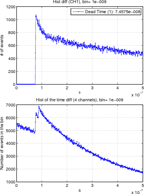
Another important advantage of splitting the beam into four parts regards the detector characteristics. As mentioned in Sect. 2.2, the SPADs used have a 75 ns dead time, i.e. after the detection of one photon event, the detector is insensitive for this time interval. The dead time limits the dynamics to higher rates when observing a bright source, and is particularly severe for quantum applications, where photon statistics must be measured. The introduced parallelism between the sub-pupils, and the consequent use of four detectors, partially overcomes this problem. Because of the statistical distribution of events over the four detectors, many events that would be otherwise lost are recovered. This effect can be clearly seen in Fig. 3, where the two cases, single detector and four-detectors, are compared. The curves are histograms of the time differences between successive photon counts, binned into units of 1 ns. The bottom curve shows the partial recovery of the otherwise lost counts at time intervals shorter than the dead time itself. Obviously, the larger the number of detectors, the smaller is the overall effect of the dead time.
|
Figure 3: ( Top) Measurement of the dead time of one SPAD. ( Bottom) Dead time for the combination of the four SPADs, showing a partial recovery of the lost counts at time intervals shorter than the dead time itself. |
| Open with DEXTER | |
The global efficiency of the system has also been estimated by taking into account the three reflections of NTT mirrors, the reflection at the pyramid, the nominal transmission of all the lenses, and the detector quantum efficiency. The result obtained is shown in Fig. 4, together with the expected sensitivity when using the three B, V, and R wide-band filters. It can be seen that the global sensitivity curve is dominated by the SPAD efficiency (Billotta et al. 2009) reaching a peak of more than 33% at 550 nm.
![\begin{figure}
\par\includegraphics[width=8cm,clip]{12862f05.eps}
\end{figure}](/articles/aa/full_html/2009/46/aa12862-09/img14.png)
|
Figure 4: Estimated global efficiency of Iqueye applied to NTT. |
| Open with DEXTER | |
From this curve, it is also possible to evaluate the expected
signal-to-noise ratio (SNR) as a function of the target magnitude.
As an example, Fig. 5 shows the calculated exposure
times needed to achieve the required SNR for a given exposure time,
in the V-band, per single SPAD, assuming a source at zenith, no moon
light, a sky brightness of 21.9 mag/arcsec![]() , a
collected FoV of 3 arcsec, and a detector dark count rate of 50 c/s.
At the faintest magnitudes, Iqueye SNR is limited by the detector
dark count and not by the night sky.
, a
collected FoV of 3 arcsec, and a detector dark count rate of 50 c/s.
At the faintest magnitudes, Iqueye SNR is limited by the detector
dark count and not by the night sky.
| Figure 5: The calculated exposure time to reach a wanted SNR in the V band. |
|
| Open with DEXTER | |
2.3 Iqueye data acquisition system
The task of the Iqueye data acquisition system (IDAS) is conceptually very simple: it must collect pulses produced from each SPAD when a photon is detected, assign a very accurate absolute time tag to each event, and store the time tags in the external memory. In reality, this is not an easy task at all, because of the stringent requirements: namely, to produce an absolute, UTC referenced time tag for each detected photons with a rms accuracy of the order of 500 ps for at least one hour of continuous operation, coping with count rates ranging from few tens of Hz up to 8 MHz.
The starting point for defining the IDAS (see Fig. 6) is the pulse produced by the SPADs once a photon is detected. As already mentioned, the SPAD used has two different outputs: a TTL one, which can sustain count rates as high as 12 MHz in the linear regime, with about 250 ps timing accuracy and a NIM one, which has a maximum linear count rate of about 2 MHz, but a much more accurate 35 ps typical timing accuracy. Since Iqueye was designed to reach a rms time tagging resolution of the order of 100 ps, the NIM output was adopted as a baseline, notwithstanding the lower possible maximum count rate, while the TTL one can be used in parallel mainly for control purposes.
![\begin{figure}
\par\includegraphics[width=9cm,clip]{12862f07.eps}
\end{figure}](/articles/aa/full_html/2009/46/aa12862-09/img16.png)
|
Figure 6: Conceptual schematic of the acquisition and timing system of Iqueye. |
| Open with DEXTER | |
Each of the 4 NIM signals is transferred from the SPADs, by means of calibrated equal electrical length coaxial cables to ensure the same electrical delay, to one of the input channels of a time to digital converter (TDC) board (CAEN V1290N, originally developed for high energy physics applications). This TDC board is nominally able to time-tag the voltage pulses on its inputs with a 24.4 ps time resolution: this very high sampling is obtained by means of a 40 MHz internal oscillator whose frequency is multiplied by 1024 by means of a phase locked loop (PLL), and a delay locked loop (DLL), providing a 40 GHz clock. Unfortunately, the quality of the internal oscillator is insufficient to satisfy the extremely severe stability requirement of our applications, for which it is necessary to obtain simultaneously both the short-term stability typical of a quartz oscillator and the long-term one assured by a primary time reference. This task could be reached by using primary time references such as hydrogen-maser clocks, which however are really expensive, difficult to handle and not available at NTT. To obtain a nearly optimal and affordable performance, we therefore focused our attention on a combination of a rubidium oscillator, a GPS receiver, and a post-processing algorithm, as described in the following.
The Iqueye time and frequency unit (ITFU), shown in Fig. 7, is based on the concept of correcting the long-term drift of the reference frequency provided by the rubidium oscillator by means of a post-processing algorithm that uses the pulse-per-second (PPS) signal provided by a mini-T Trimble GPS receiver. The GPS also provides the synchronization to UTC. The ITFU uses a Stanford Research System FS275 rubidium oscillator that produces a 10 MHz sinusoidal signal, that then is converted to a 40 MHz TTL signal by means of a frequency multiplication by a Tektronics AFG3251 pulse generator and a signal generator. The TTL signal represents the input to the IDAS. The rubidium atomic clock is the optimal trade-off in terms of performance and costs, ensuring good stability for medium lengths of time (<104 s). The most stable and high performance clock would be the hydrogen maser, but its cost exceeds the available resources.
![\begin{figure}
\par\includegraphics[width=8cm,clip]{12862f08.eps}
\end{figure}](/articles/aa/full_html/2009/46/aa12862-09/img17.png)
|
Figure 7: Block diagram of the Iqueye time and frequency unit, which provides the frequency standard to the experiment. OCXO is an acronym for Oven-Controlled Crystal Oscillator. |
| Open with DEXTER | |
As shown in Fig. 7, the rubidium oscillates in
free-running mode, that is it is not disciplined by an external
reference because this would worsen the phase noise. The tests
performed at the Laboratory of Time & Frequency
of the
Astronomical Observatory of Cagliari (OAC) using a primary standard
caesium clock as reference, showed that the rubidium accumulates a
phase drift of approximately 65 ns after one hour, and 160 ns
after
two hours. However, by removing such linear drift, only a residual
stochastic phase error remains, whose rms value is shorter than
50 ps for a duration of more than 1000 s (see for example
Fig. 8). For the Allan variance, it has a minimum
corresponding to
![]() after 104 s.
after 104 s.
By adding the rms time errors in the SPADs (35 ps), in the electronics chain (50 ps), and in the residual phase error (50 ps rms for one hour of observation) to the internal sampling discretization (24.4 ps), a total rms time error of approximately 100 ps is obtained, which satisfies the design requirements. This is the level of relative rms time accuracy that we can reach with Iqueye for one-hour observations.
![\begin{figure}
\par\includegraphics[width=8cm,clip]{12862f09.eps}
\end{figure}](/articles/aa/full_html/2009/46/aa12862-09/img19.png)
|
Figure 8: Residuals of the rubidium oscillator pulse per second (PPS) versus the Astronomical Observatory of Cagliari caesium oscillator PPS after removal of the linear phase drift. The abscissa spans over 1000 s. |
| Open with DEXTER | |
To remove the linear drift and obtain the UTC synchronization while
operating at the telescope, Iqueye uses the PPS signal provided by a
GPS receiver. These PPSs are given to the CAEN board via a TTL/NIM
converter as input pulses on a fifth channel, and are processed by
the board, in the same way as photon pulses from the 4 SPADs are
treated. The CAEN internal oscillator is disabled, and the board
uses the 40 MHz frequency provided by the ITFU. Post-processing
algorithms estimate and remove the rubidium oscillator phase drift
using the GPS PPS, and finally the UTC corrected time tags are made
available for further processing. To determine the uncertainty in
the start time, the start signal is provided by the PC controlling
the data acquisition, whose system clock is disciplined by the
Network Time Protocol with a typical uncertainty of few
milliseconds. However, the true start of the acquisition is given by
the first PPS encountered in the data string, and therefore has a
rms uncertainty of approximately ![]() 25 ns as typically associated
with a good quality single frequency GPS receiver. However, owing to
the linear drift interpolation, the error associated with the
starting time decreases with the number of acquired PPS: by means of
simple calculations, it can be verified that after one hour of
observation this error decreases to 0.4 ns rms. Therefore,
considering the 100 ps relative time accuracy for an acquisition of
one hour, an absolute rms time accuracy with respect to UTC of
shorter than 0.5 ns is obtained.
25 ns as typically associated
with a good quality single frequency GPS receiver. However, owing to
the linear drift interpolation, the error associated with the
starting time decreases with the number of acquired PPS: by means of
simple calculations, it can be verified that after one hour of
observation this error decreases to 0.4 ns rms. Therefore,
considering the 100 ps relative time accuracy for an acquisition of
one hour, an absolute rms time accuracy with respect to UTC of
shorter than 0.5 ns is obtained.
A limitation of the TDC board is that it returns a time-tag value
digitized at 21 bits. Given the 24.4 ps time digitization, the
longest unambiguous time interval is only
![]()
![]() s,
while all times longer than this interval have an initial phase
s,
while all times longer than this interval have an initial phase
![]() ,
where N is an integer to be determined. To realize
this so-called ``de-rollover'' process, we feed the TDC board with
an external 20 kHz reference pulse, which allows us to determine the
value of N and recover the initial phase.
,
where N is an integer to be determined. To realize
this so-called ``de-rollover'' process, we feed the TDC board with
an external 20 kHz reference pulse, which allows us to determine the
value of N and recover the initial phase.
The overall system was designed with a modular approach. The TDC board is equipped with 16 inputs: presently only six of them are used, so that a further expansion of the number of detectors is possible with no need to upgrade the IDAS. Moreover, the TDC board is lodged inside a standard crate, which can host additional boards all connected to the same VME bus. In practice, other TDC boards can be added, if necessary, with no need to modify the present system.
A dedicated server manages all the data exiting the TDC. This server
is connected to the VME bus inside the CAEN crate. From here,
through a bridge and an optical fiber, the data are sent to the
acquisition server, with an approximate maximum speed of 60 Mb/s.
This is the present bottleneck that limits the maximum count rate of
the system, but it can be overcome as discussed in the final
considerations. The user interface, which is implemented by means of
a second server, has been developed as a Java multitasking code: it
allows the acquisition control and the data storage, the control of
each instrument subsystem and in particular of all the mechanisms,
it can perform several real-time quick-look statistical analyses of
the acquired data, and allows us to read and store the images of the
stellar field around the selected object acquired by the field
camera. These images can be used for an a-posteriori analysis of
guiding errors and sky conditions. The storage capability is
approximately 2 TB: all the data are recorded in a 6 SATA disks
raid6 configuration, to ensure both redundancy and speed in
accessing the database. All the electronics equipment is mounted
into a standard 19
![]() rack that can be placed into the NTT Nasmyth
focus room, just under Iqueye's optics. The whole system is
connected to the NTT IP network, so that the instrument can be
remotely controlled.
rack that can be placed into the NTT Nasmyth
focus room, just under Iqueye's optics. The whole system is
connected to the NTT IP network, so that the instrument can be
remotely controlled.
We remark that the stored data contain long strings of time tags. With these data, all possible types of post-processing analysis (i.e., calculations of autocorrelation, cross-correlation, FFT, power spectra, periodograms, light curves) can be done without affecting the integrity of the original data. For instance, the events can be sorted by the most convenient time bin for the specific scientific analysis without losing any original information.
The main characteristics and performance of Iqueye are summarized in Table 2.
Table 2: Main characteristics describing the performance of Iqueye applied to NTT.
3 Preliminary astronomical results of Iqueye
We performed our observations at the NTT on 14-19 January 2009, operating Iqueye across its entire range of count rates, from extremely faint to very bright sources. The capability of our apparatus to time-tag photons with extremely accurate precision over a very wide dynamic range was demonstrated convincingly. We provide two examples of the single photon capabilities, leaving discussion of the astronomical results to future papers. The first example, the pulsar of the Crab Nebula, illustrates the capabilities of Iqueye in conventional high speed photometry. Figure 9 shows a string of individual pulses from the pulsar after transmission through a linear polarizer, with the counts binned in 3.3 ms time bins, which is one tenth of the pulsar period. The great sensitivity of Iqueye is clearly evident: it is able to resolve to high accuracy the 33 ms single periods of this weak V = 16.5 object. Figure 10 shows the Crab pulsar light curve obtained by folding only 1 s integration counts with a 33.627 ms period and two different time bins: 0.07 ms on the left, and 0.6 ms on the right. One second of time is more than sufficient to obtain reliable information of this light curve.
![\begin{figure}
\par\includegraphics[width=8cm,clip]{12862f10.eps}
\end{figure}](/articles/aa/full_html/2009/46/aa12862-09/img23.png)
|
Figure 9: Individual counts from the Crab Nebula pulsar, with 0.33 ms (1/10 of the period) bin size. The average count rate per time bin is given in the box. |
| Open with DEXTER | |
![\begin{figure}
\par\includegraphics[width=8cm,clip]{12862f11.eps}\par\includegraphics[width=8cm,clip]{12862f12.eps}
\end{figure}](/articles/aa/full_html/2009/46/aa12862-09/img24.png)
|
Figure 10: Crab pulsar light curves obtained with one second of acquisition. The same data have been binned with two different time bins: 0.07 ms ( top) and 0.6 ms ( bottom). |
| Open with DEXTER | |
The second example illustrates how to quantum astronomy can be achieved by the calculation of g(2), i.e., the second order correlation function (Barbieri et al. 2009a; LeBohec et al. 2008; Dravins et al. 2005; Foellmi 2009) using the present technology of Iqueye. In particular, we verified the capability of Iqueye to perform the measurement of g(2)(d) as a function of the relative distance d of the collecting apertures, thus confirming its effectiveness as an intensity interferometer (Hanbury Brown 1974).
The bright star ![]() Ori (HD 37743, V = 1.8, SpT = O9.5Ib, with
emission lines) was observed on January 21
Ori (HD 37743, V = 1.8, SpT = O9.5Ib, with
emission lines) was observed on January 21![]() ,
2009 at UTC
(start) 01h06m24s for 1h8m through the wide band B and neutral
density 2 filters using the 5.2 arcsec pinhole. The star was chosen
because it appears in the list of stars observed with the intensity
interferometer at Narrabri (Hanbury Brown et al. 1974). The authors quoted a
zero baseline correlation coefficient
,
2009 at UTC
(start) 01h06m24s for 1h8m through the wide band B and neutral
density 2 filters using the 5.2 arcsec pinhole. The star was chosen
because it appears in the list of stars observed with the intensity
interferometer at Narrabri (Hanbury Brown et al. 1974). The authors quoted a
zero baseline correlation coefficient
![]() ,
very
far from the value of 1 expected from a single unresolved star.
Their explanation of the difference was that it is caused by the
limited the resolution of the stellar disk, which corresponds to an
angular extent of the order of 0.5 mas for a uniformly illuminated
disk. It is well known (see Mason et al. (1998) and the Washington Double
Star Catalog
,
very
far from the value of 1 expected from a single unresolved star.
Their explanation of the difference was that it is caused by the
limited the resolution of the stellar disk, which corresponds to an
angular extent of the order of 0.5 mas for a uniformly illuminated
disk. It is well known (see Mason et al. (1998) and the Washington Double
Star Catalog![]() ) that the
) that the ![]() Ori is a
triple star, the secondary (
Ori is a
triple star, the secondary (![]() Ori B, V = 4.20, SpT = B0III,
flux
Ori B, V = 4.20, SpT = B0III,
flux
![]() )
being approximately 2
)
being approximately 2
![]() 5 distant to the
south east, and therefore just at the edge of the used pinhole. The
tertiary weaker component is too far to be of concern in our data.
5 distant to the
south east, and therefore just at the edge of the used pinhole. The
tertiary weaker component is too far to be of concern in our data.
The method we have used to calculate
g(2)(d) consists of
correlating the event time-tag strings obtained by each SPAD,
searching for coincidences among every pair of possible
combinations. In effect, the photons collected by each SPAD arrive
from four different sub-pupils of the NTT aperture: this allows us
to consider the system as four parallel smaller telescopes, each
focused on one SPAD. Clearly, the collecting area of each
sub-aperture is small and the baseline distances d are fixed even
though they rotate on the sky during the exposure time, because of
the telescope Alt-Az mount; we therefore did not expect to obtain
significant astrophysical results. Since the separation between the
telescope sub-apertures is small compared with the Narrabri
telescopes, we expected that
![]() ,
and that
g(2)(d) is slightly smaller than 1. This
was, first, because the stellar disk cannot be resolved by the small
baselines available with this setup, and second, because the
secondary star at the edge of the field of view should contribute a
minimum amount of additional flux, since seeing is occasionally
scattering a fraction of its light outside the pinhole. Finally,
because the maximum overall photon rate that can be handled with the
present equipment is approximately 10 times lower than the minimum
rate necessary to achieve an acceptable signal-to-noise ratio (see
Hanbury Brown 1974) for detecting second order effects. We therefore
performed this experiment in preparation for an observation with two
larger and more widely separated telescopes such as two VLTs, and
and improved Iqueye now under construction. Nevertheless, we believe
that these preliminary results are of sufficient interest to be
expounded here because, to our knowledge, they represent the first
attempt to perform intensity interferometry by time-tagging each
detected photon and then post-processing the data, and thus avoiding
real-time analog or digital correlators, which do not preserve data
for all the original photon-events.
,
and that
g(2)(d) is slightly smaller than 1. This
was, first, because the stellar disk cannot be resolved by the small
baselines available with this setup, and second, because the
secondary star at the edge of the field of view should contribute a
minimum amount of additional flux, since seeing is occasionally
scattering a fraction of its light outside the pinhole. Finally,
because the maximum overall photon rate that can be handled with the
present equipment is approximately 10 times lower than the minimum
rate necessary to achieve an acceptable signal-to-noise ratio (see
Hanbury Brown 1974) for detecting second order effects. We therefore
performed this experiment in preparation for an observation with two
larger and more widely separated telescopes such as two VLTs, and
and improved Iqueye now under construction. Nevertheless, we believe
that these preliminary results are of sufficient interest to be
expounded here because, to our knowledge, they represent the first
attempt to perform intensity interferometry by time-tagging each
detected photon and then post-processing the data, and thus avoiding
real-time analog or digital correlators, which do not preserve data
for all the original photon-events.
The method that we have followed to compute
g(2)(d) values
originates from (Beck 2007), who used two different coincidence
detection techniques: one using time-to-amplitude converters, which
is affected by dead-time problems as are our SPADs, and another
using a logic circuit that has essentially no dead-time. The formula
for the calculation of
g(2)(d) is
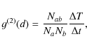
where Na and Nb are the total counts on detectors a and b respectively, and Nab is the number of coincidences, which is the number of simultaneous event detections in a and b within a coincidence window
Table 3:
Values of
![]() obtained from one
hour observation of the bright star
obtained from one
hour observation of the bright star ![]() Ori, for each pair a,bof sub-apertures, assuming a time coincidence window
Ori, for each pair a,bof sub-apertures, assuming a time coincidence window
![]() ps.
ps.
Determining the Na and Nb values is straightforward, but this
is not the case for Nab. The calculation of the correlation
between the channels is not a trivial task when the coincidence
window ![]() is very small and the observing time
is very small and the observing time ![]() is
very long. To illustrate the difficulty, we consider sampling one
hour of observations using the smallest coincidence window allowed
by Iqueye, 24.41 ps, which corresponds using about
is
very long. To illustrate the difficulty, we consider sampling one
hour of observations using the smallest coincidence window allowed
by Iqueye, 24.41 ps, which corresponds using about
![]() windows: after assigning one bit to any of these windows
(``0'' when there is no coincidence, ``1'' when there is a
coincidence), each of the files to be correlated would have a size
of about 18 TB.
windows: after assigning one bit to any of these windows
(``0'' when there is no coincidence, ``1'' when there is a
coincidence), each of the files to be correlated would have a size
of about 18 TB.
We therefore devised an ad hoc Matlab algorithm based on the
principle that if two events are separated by a time difference m,
then the correlation vector at position m must be increased by 1.
The algorithm was optimized to work with time bins of
![]() ps, where N is a non-negative integer, because these choices
of bin-size minimize the computation time. As input, this routine
needs the files that collect the time tags: even if the size of
these data files remains large, the algorithm performs the
calculation in a reasonable time, even without the use of
supercomputers. In the specific case of
ps, where N is a non-negative integer, because these choices
of bin-size minimize the computation time. As input, this routine
needs the files that collect the time tags: even if the size of
these data files remains large, the algorithm performs the
calculation in a reasonable time, even without the use of
supercomputers. In the specific case of ![]() Ori, approximately
Ori, approximately
![]() photons were detected, and the time tags were
collected in 7771 files each of 10 MB, for a total of 78 GB.
Processing all these data with the smallest possible 24.41 ps
coincidence windows lasted only about half a day on a 32 GB RAM four
processor machine.
photons were detected, and the time tags were
collected in 7771 files each of 10 MB, for a total of 78 GB.
Processing all these data with the smallest possible 24.41 ps
coincidence windows lasted only about half a day on a 32 GB RAM four
processor machine.
To obtain a clearer understanding of the results and in particular
estimate the statistical errors affecting the determination of
g(2), the entire string of 7771 files was divided into seven
clusters of 1000 files each (the remaining 771 files were
discarded), and the value of
g(2)(d) was calculated for each
cluster by setting a coincidence window
![]() ps. From
these values, the average
ps. From
these values, the average
![]() was
calculated together with its standard deviation. The results
obtained from this analysis are summarized in Table 3.
The table shows the pairs of SPADs used in the calculation, each
SPAD being represented with a capital letter; not all combinations
are shown because in the cross-correlation, pairs A-B and B-A give
identical results. The flux-weighted distance d between the two
apertures is given in the second column, and the third column
provides an indicative resolving angle computed as
was
calculated together with its standard deviation. The results
obtained from this analysis are summarized in Table 3.
The table shows the pairs of SPADs used in the calculation, each
SPAD being represented with a capital letter; not all combinations
are shown because in the cross-correlation, pairs A-B and B-A give
identical results. The flux-weighted distance d between the two
apertures is given in the second column, and the third column
provides an indicative resolving angle computed as
![]() ,
where the effective wavelength
,
where the effective wavelength
![]() nm has
been taken to be the center of the observing filter. The last two
columns indicate the value of
nm has
been taken to be the center of the observing filter. The last two
columns indicate the value of
![]() and its
standard deviation respectively. Note that the last column is not
the true error in the value of
g(2)(d), but simply the standard
deviation of the average value
and its
standard deviation respectively. Note that the last column is not
the true error in the value of
g(2)(d), but simply the standard
deviation of the average value
![]() ,
calculated by considering the seven independent 1000 file clusters.
,
calculated by considering the seven independent 1000 file clusters.
It is clear that the measurement and the algorithm are very stable, with relative fluctuations of g(2)(d) smaller than 1%. In addition, when all the 7771 files are processed together, the g(2)(d) values obtained differ from those of the 1000 clusters by less than 1%. Although the results are internally consistent, and even given values slightly less than 1 as expected a priori, we recall that this analysis was not designed to provide a true measurement, but simply to validate the method. The small aperture of the telescope and the already mentioned limitation in the dynamic range of the electronics used in January 2009, provided a signal-to-noise ratio too low to achieve significant astrophysical results.
4 Future developments
During three years of laboratory and telescope work, we have shown the advantages of using single photon avalanche diodes operated in Geiger mode for high time-resolution astrophysical problems. In particular, the superior quality of the La Silla site and the performance of NTT have allowed us to obtain a significant amount of scientific data that is now being analyzed. The detectors we have employed have shown good performances in terms of quantum efficiency, time tagging accuracy, high dynamic range, modest dark count, reliability and ease of operation. In contrast, its disadvantages include a the single-pixel small-area configuration, a long dead-time preventing us from exceeding a count rate of approximately 14 MHz per SPAD, and a non-negligible afterpulsing effect.
Several improvements remain possible for Iqueye. Iqueye is now being fitted with custom lenses to achieve a higher concentration of the light on the SPAD. In addition, four filter wheels, one per SPAD, are being added, to allow simultaneous multispectral analysis. The throughput at the NIM connector could be increased toward the theoretical limit imposed by the dead time, which could also be shortened; MPD is already attempting to find the optimal compromise between deadtime, timing jitter, and afterpulsing specifically for the foreseen astronomical applications. In conjunction with CAEN, we propose to develop a dedicated TDC board with the acquisition computer directly inside the VME crate. The technology of single photon detectors is also rapidly improving, driven by other powerful users such as the community of classical and quantum communications.
We note that the instrument we have described, suitably adapted, could be immediately applied to the VLT, in particular for HBT intensity interferometry. However, by the time that the E-ELT is ready, photon-counting arrays with imaging capabilities may be available, greatly improving the performance of this type of instrumentation. As a final consideration, accurate time-keeping is a fundamental variable for this type of applications: first class observatories, in particular the VLT and the E-ELT, should be equipped with primary time standards as all VLBI stations are.
5 Conclusions
The main conclusions of our present study can be summarized as follows.
- 1.
- A new extremely fast photon-counting photometer, Iqueye, has been tested at NTT, where its superb potentiality for observing fast variable objects, such as pulsars, was clearly demonstrated. These tests permitted hours of uninterrupted observations with an absolute timing accuracy superior to 0.5 ns.
- 2.
- Iqueye paves the way toward the realization of a truly ``quantum'' photometer for the 42 m E-ELT.
- 3.
- The results already obtained by Iqueye attest that a quantum photometer at the E-ELT will be able to measure second and higher order correlation functions, so opening the road to new tools of investigation of the Universe.
Iqueye was constructed with funds provided by the Italian Ministry of University and Research, the University of Padova, and the National Institute for Astrophysics through the PRIN 2006 program; by the European Community through the Harrison Project for the scientific exploitation of the Galileo GNSS; and by Fondazione CARIPARO through the Project of Excellence 2006. The authors wish to express gratitude to ESO who granted technical time at NTT for testing Iqueye and covered part of the team travel expenses. Finally, a sincere acknowledgement is due to La Silla personnel, who participated very actively in the observational campaign and made a substantial contribution to the success of the instrument testing.
References
- OWL Concept Design Report 2005, Tech. rep., ESO document OWL-TRE-ESO-0000-0001 Issue 2
- Barbieri, C., Da Deppo, V., D'Onofrio, M., et al. 2006, in The scientific requirements for extremely large telescopes, ed. P. Whitelock, B. Leibundgut, & M. Dennefeld, IAU Symp., 232, 506
- Barbieri, C., Dravins, D., Occhipinti, T., et al. 2007a, J. Mod. Opt., 54, 191 [NASA ADS] [CrossRef]
- Barbieri, C., Naletto, G., Occhipinti, T., et al. 2007b, Mem. SAIt. Suppl., 11, 190
- Barbieri, C., Daniel, M., de Wit, W., et al. 2009a, New Astrophysical Opportunities Exploiting Spatio-Temporal Optical Correlations, Science white paper prepared for the Astro2010 Decadal Review, available at [arXiv:0903.0062]
- Barbieri, C., Naletto, G., Occhipinti, T., et al. 2009b, J. Mod. Opt., 56, 261 [NASA ADS] [CrossRef]
- Barbieri, C., Naletto, G., Verroi, E., et al. 2009c, in Science with the VLT in the ELT Era, Astrophysics and Space Science Proceedings, 249
- Beck, M. 2007, J.O.S.A., 24, 2972 [CrossRef]
- Billotta, S., Belluso, M., Bonanno, G., et al. 2009, J. Mod. Opt., 56, 273 [NASA ADS] [CrossRef]
- Boiko, D., Gunther, N., Brauer, N., et al. 2009, New J. Phys., 11, 013001 [CrossRef] (7 pages)
- Cova, S., Ghioni, M., Lotito, A., Rech, I., & Zappa, F. 2004, J. Mod. Opt., 51, 1267 [NASA ADS]
- Datte, P., Birkbeck, A., Beuville, E., et al. 1999, Nucl. Instrum. Methods Phys. Res. A, 421, 576 [NASA ADS] [CrossRef]
- Dravins, D. 2008, in High Time Resolution Astrophysics, ed. D. Phelan, O. Ryan, & A. Shearer, Ap&SS Library, 315, 95
- Dravins, D., Barbieri, C., Da Deppo, V., et al. 2005, QuantEYE quantum optics instrumentation for astronomy. OWL Instrument Concept Study, Tech. rep., ESO, Document OWL-CSR-ESO-00000-0162
- Dravins, D., Barbieri, C., Fosbury, R., et al. 2006, in The scientific requirements for extremely large telescopes, ed. P. Whitelock, B. Leibundgut, & M. Dennefeld, IAU Symp., 232, 502
- Foellmi, C. 2009, A&A, submitted for publication, abstract available at http://arxiv.org/abs/0901.4587
- Glauber, R. 1963, Phys. Rev., 131, 2766 [NASA ADS] [CrossRef]
- Hanbury Brown, R. 1974, The intensity interferometer. Its applications to astronomy (London: Taylor & Francis)
- Hanbury Brown, R., Davis, J., & Allen, L. 1974, MNRAS, 167, 121 [NASA ADS]
- LeBohec, S., Barbieri, C., de Wit, W., et al. 2008, in Optical and Infrared Interferometry, ed. M. Schöller, W. C. Danchi, & F. Delplancke, SPIE Proc., 7013, 70132E
- Mason, B., Gies, D., Hartkopf, W., et al. 1998, AJ, 115, 821 [NASA ADS] [CrossRef]
- Michalet, X., Siegmund, O., Vallerga, J., et al. 2006a, in Optical Biopsy VI, ed. R. Alfano, & A. Katz, SPIE Proc., 6092, 141
- Michalet, X., Siegmund, O., Vallerga, J., et al. 2006b, J. Mod. Opt., 54, 239 [NASA ADS] [CrossRef]
- Naletto, G., Barbieri, C., Dravins, D., et al. 2006, in Ground-Based and Airborne Instrumentation For Astronomy, SPIE 6269, 62691W-1/9
- Naletto, G., Barbieri, C., Occhipinti, T., et al. 2007, in Photon counting applications, Quantum Optics, and Quantum Cryptography, SPIE, 6583, 65830B-1/14
- Niclass, C., Favi, C., Kluter, T., Gersbach, M., & Charbon, E. 2008, IEEE J. of Solid-State Circuits, 43, 2977 [CrossRef]
- Siegmund, O., Vallerga, J., McPhate, J., & Tremsin, A. 2004, in UV and Gamma-Ray Space Telescope Systems, ed. G. Hasinger, & M. Turner, SPIE Proc., 5488, 789
- Siegmund, O., Vallerga, J., Jelinsky, P., Weiss, S., & Michalet, X. 2005, IEEE Nuclear Science Symposium Conference Record, N14-55, 448
Footnotes
- ... 21.9 mag/arcsec
![[*]](/icons/foot_motif.png)
- Data for La Silla were taken from: http://www.vt-2004.org/gen-fac/pubs/astclim/lasilla/index.html
- ... Catalog
- The Washington Double Star Catalogue is maintained at the U.S. Naval Observatory http://ad.usno.navy.mil/wds/wds.html
All Tables
Table 1: Main characteristics of the filters/polarizers available on the two Iqueye filter wheels.
Table 2: Main characteristics describing the performance of Iqueye applied to NTT.
Table 3:
Values of
![]() obtained from one
hour observation of the bright star
obtained from one
hour observation of the bright star ![]() Ori, for each pair a,bof sub-apertures, assuming a time coincidence window
Ori, for each pair a,bof sub-apertures, assuming a time coincidence window
![]() ps.
ps.
All Figures
|
|
Figure 1: Schematic view of Iqueye optical design. |
| Open with DEXTER | |
| In the text | |
| |
Figure 2:
Encircled energy plot showing the energy distribution on
the 100 |
| Open with DEXTER | |
| In the text | |
|
|
Figure 3: ( Top) Measurement of the dead time of one SPAD. ( Bottom) Dead time for the combination of the four SPADs, showing a partial recovery of the lost counts at time intervals shorter than the dead time itself. |
| Open with DEXTER | |
| In the text | |
|
|
Figure 4: Estimated global efficiency of Iqueye applied to NTT. |
| Open with DEXTER | |
| In the text | |
| |
Figure 5: The calculated exposure time to reach a wanted SNR in the V band. |
| Open with DEXTER | |
| In the text | |
|
|
Figure 6: Conceptual schematic of the acquisition and timing system of Iqueye. |
| Open with DEXTER | |
| In the text | |
|
|
Figure 7: Block diagram of the Iqueye time and frequency unit, which provides the frequency standard to the experiment. OCXO is an acronym for Oven-Controlled Crystal Oscillator. |
| Open with DEXTER | |
| In the text | |
|
|
Figure 8: Residuals of the rubidium oscillator pulse per second (PPS) versus the Astronomical Observatory of Cagliari caesium oscillator PPS after removal of the linear phase drift. The abscissa spans over 1000 s. |
| Open with DEXTER | |
| In the text | |
|
|
Figure 9: Individual counts from the Crab Nebula pulsar, with 0.33 ms (1/10 of the period) bin size. The average count rate per time bin is given in the box. |
| Open with DEXTER | |
| In the text | |
|
|
Figure 10: Crab pulsar light curves obtained with one second of acquisition. The same data have been binned with two different time bins: 0.07 ms ( top) and 0.6 ms ( bottom). |
| Open with DEXTER | |
| In the text | |
Copyright ESO 2009
Current usage metrics show cumulative count of Article Views (full-text article views including HTML views, PDF and ePub downloads, according to the available data) and Abstracts Views on Vision4Press platform.
Data correspond to usage on the plateform after 2015. The current usage metrics is available 48-96 hours after online publication and is updated daily on week days.
Initial download of the metrics may take a while.