---

A&A 508, 53-62 (2009)

Simulating weak lensing of CMB maps

S. Basak - S. Prunet - K. Benabed

Institut d'Astrophysique de Paris, CNRS, UMR 7095, 98 bis Boulevard Arago, 75014 Paris, France

Received 11 June 2009 / Accepted 7 September 2009

Abstract
Aims. Accurate predictions of cosmic microwave background (CMB) anisotropies and polarization are required for analyzing future CMB data sets, which ultimately require accurately simulated lensed maps.
Methods. We present a fast, arbitrarily accurate method to simulate the effect of gravitational lensing of the CMB anisotropies and polarization fields by large-scale structures on arbitrarily spaced grid points over a unit sphere using a non-equispaced fast Fourier transform (NFFT).
Results. The angular power spectrum of the simulated lensed CMB map, particularly the B-mode of polarization, agrees extremely well with analytical predictions. The analytical derivation of CMB-lensed spectra is based on non-trivial, partially resummed perturbative expansions of the correlation functions, for which our simulations therefore provide an accurate numerical validation. We demonstrate the efficiency and accuracy of the method and exhibit their dependence on the algorithm parameters. Lensed CMB maps simulated in this method are a useful tool for the analysis and interpretation of upcoming CMB experiments, such as PLANCK and ACT. Our code is available on request.

Key words: cosmic microwave background

1 Introduction

Weak lensing effects on the cosmic microwave background (CMB) temperature and polarization anisotropies has been proposed as a probe of the total matter distribution in large-scale structures (LSS) between us and the surface of last scattering (Hu 2000; Seljak 1996; Benabed et al. 2001; Hu 1999; Hirata & Seljak 2003a; Kesden et al. 2002; Guzik et al. 2000; Lewis 2005; Hirata et al. 2004; Smith et al. 2007; Lewis & Challinor 2006; Van Waerbeke et al. 2000; Hu & Tegmark 1999; Zaldarriaga & Seljak 1999; Kesden et al. 2003; Challinor & Lewis 2005; Hirata & Seljak 2003b; Zaldarriaga & Seljak 1998; Blanchard & Schneider 1987). Although sensitive to the cumulative distribution of matter, it is quite complementary to other probes of the matter distribution of the LSS. It does not suffer from bias effects (such as e.g. galaxy redshift surveys, Lyman- forest), or incorrect determination of the redshift sources (e.g., as cosmic shear measurements on galaxies). In addition, because of the high redshift of the source (last scattering surface) and the lensing efficiency function, weak lensing of CMB anisotropies is mostly sensitive to large-scale structures that remain (mainly) in the linear regime, which makes it a very useful tool for cosmology, in particular for constraining the properties of neutrinos (Perotto et al. 2006; Lesgourgues et al. 2006).

Unlike shear measurements of galaxies, where the (reduced) shear field is directly sampled by measurement of galaxy ellipticities, measuring weak lensing effects on the CMB is complicated by the intrinsic stochasticity of the source. However, theoretical arguments lead us to think that CMB anisotropies are highly Gaussian (Linde 1982; Guth 1981; Albrecht & Steinhardt 1982), which has been confirmed on the data, at large scales, using different non-Gaussianity estimators (probability distribution function, bispectrum, wavelet skewness and kurtosis, Minkowski functionals). These properties of the CMB anisotropies can be used to help disentangle the stochastic properties of the (unlensed) CMB anisotropies from the stochastic properties of the lens (i.e., the LSS) since the lensing effect induces small specific non-Gaussian features in the CMB maps. In particular, it correlates the anisotropies locally with their gradient (Cooray & Hu 2002,2001a,b; Seljak 1996; Cooray et al. 2000), which led to the development of specific estimators of the lensing potential field and its power spectrum (Hu & Okamoto 2002; Hirata & Seljak 2003b,a; Okamoto & Hu 2003).

Weak lensing of the CMB anisotropies by LSS was measured in WMAP data (Smith et al. 2007) by its cross-correlation with a high-redshift radio galaxy catalog. Although only marginally detectable in WMAP data because of its noise level, CMB lensing should be measured with a high signal-to-noise ratio by Planck with temperature anisotropies alone (Cooray & Hu 2002; Hu & Okamoto 2004) without needing to rely on any external data set. However, to carry out this measurement on realistic CMB data, the impact of instrumental (anisotropic beams, missing data, correlated noise) and astrophysical (e.g., Galaxy contamination, point sources, etc.) systematic effects on the CMB lensing estimators must be studied with great care.

The power spectra (temperature and polarization) can be computed, using a simple Taylor expansion at large scales (Hu 2000), or a more clever resummation scheme at smaller scales where the displacement field amplitude is comparable to the wavelength of the anisotropies (Challinor & Lewis 2005). For smaller scales, or to investigate the different systematics described above, the development of fast, accurate methods for simulating the lensed CMB maps are needed.

This simulation comes in two distinct parts. On the one hand, an accurate simulation of the large-scale structure induced lensing deflection field is needed. On the other hand, one needs a method to apply this deflection field to an unlensed, simulated CMB. We do not consider the first part of this program, because approximating the lensing effect with a single lens plane in the so-called Born approximation (Hu 2000) has been shown to provide an excellent approximation, both for temperature and polarization anisotropies. In this case, the simulation of lensed CMB maps reduces to an accurate resampling of the unlensed anisotropies at displaced positions. To solve this last problem, several technical solutions were implemented. In the publicly distributed Lenspix code, different possibilities are available, namely

• brute-force resampling by direct resummation of spherical harmonics at displaced positions (being slow, but very accurate, this option should be considered as the ``benchmark'' for all other resampling methods);
• resampling on locally Cartesian grids with subsequent polynomial interpolation.

For the second option, an interesting speed-up was proposed by Hirata et al. (Hirata et al. 2004) by noting that a band-limited signal in spherical harmonics can be recast as a band-limited signal in regular Fourier modes on , thus allowing a fast resampling of the signal on a cartesian grid using 2-d fast Fourier transforms (FFT hereafter). This idea was implemented by Das & Bode (2008) in their simulation of gravitational lensing of the CMB temperature field over a large area of the sky.

In this paper, we investigate a development of Hirata's idea (Das & Bode 2008; Hirata et al. 2004), where the oversampling plus polynomial interpolation is replaced by an approximate (but arbitrarily accurate) FFT resampling at irregularly spaced grid points.

The remainder of this paper is organized as follows. In Sect. 2 we briefly describe the resampling technique (hereafter NFFT), and the weak lensing of primary CMB fields in Sect. 3. We also demonstrate how the remapping of CMB fields onto the surface of the unit sphere is equivalent to the remapping of the same field on the surface of a 2-d torus. Section 4 describes the simulation procedure for lensed CMB fields, which applies NFFT to the surface of a 2-d torus. Finally, we summarize our results in Sect. 5.

2 Non-equispaced fast Fourier transform (NFFT)

The fast Fourier transform for non-equispaced grid points (NFFT) is a generalization of FFT (Kunis & Potts 2008; Fourmont 2003). The essential idea is that the reproducing kernel of the standard FFT is approximated by using a window function of specific properties. We assume that we know a function f by means of N evaluations f_kin the frequency domain. According to NFFT, the Fourier transform of that function evaluated at M non-equispaced grid points in the spatial domain can be written as,

Here the window function has compact support , and its Fourier transform assumes small values outside some interval . The parameter is the oversampling factor and it is required to avoid the aliasing error. A good choice of is 2, although is sufficient to achieve high accuracy. We also note that has to be chosen slightly smaller than . Since the evaluation of the summation over k requires an equispaced FFT of length , must be well localized in k-space to avoid the aliasing error with minimal computational cost. On the other hand, the summation over m can be evaluated with minimum truncation error if the window function is well localized in the spatial domain. Hence, the efficient evaluation of on irregularly spaced grid points requires a window function that is well localized in both space and frequency domain. It has a computational complexity , where K is the number of terms considered in the spatial approximation, M is the number of real space samples, and N is the number of Fourier modes. Among a number of window functions (Gaussian, B-spline, sinc-power, Kaiser-Bessel), the Kaiser-Bessel function is found to provide the most accurate results. It has been shown that for a fixed oversampling factor , the approximation error decays exponentially with K(Kunis & Potts 2008; Fourmont 2003).

3 Weak lensing of CMB

The CMB radiation field is characterized completely by its temperature anisotropy, , and polarization, , in every direction of the sky. Since temperature anisotropy is a spin-0 field on the sphere, it can be conveniently expanded in terms of spin-0 spherical harmonics,

The polarization field can be described by the Stokes parameters, and , with respect to a particular choice of coordinate system on the sky. One can conveniently combine the Stokes parameters into a single complex quantity representing the polarization, . Because of its transformation properties under rotations, the polarization P is a spin-2 field on the sphere. One may thus expand in terms of spin-2 spherical harmonics, (Thorne 1980; Goldberg et al. 1967; Newman & Penrose 1966; Zaldarriaga & Seljak 1997) as

In the above equation, , where E_lm and B_lm are the electric and magnetic modes of the polarization field in harmonic space.

Weak lensing induces a deflection field , i.e., a mapping between the direction of a given light ray on the last scattering surface and the direction in which we observe it. Since the deflection field is a vector field on the sphere, it can be decomposed into gradient-free and curl-free components in the most general form as

where and are two scalar fields on the sphere, and is the covariant antisymmetric tensor of rank 2 on the unit sphere. In terms of null basis vectors defining a diad on the unit sphere, can be expressed as

The gradient-free component can be ignored because it is negligible in most cases (Cooray & Hu 2002) and is exactly zero for the Born approximation that adopt here, as this term is generated only by the lens-lens couplings. In the Born approximation, the lensing deflection is calculated along the unlensed line of sight, so the lensed map is a local function of the deflection vector , where is the lensing potential. This projected potential is related to the three-dimensional (3-d) gravitational potential in terms of

where D is the comoving coordinate distance along the line of sight, is the comoving angular diameter distance associated with D, and is the comoving coordinate distance to the last scattering surface.

As for the CMB temperature anisotropy, the lensing potential transforms like a spin-zero field on the sphere. Hence, it may also be expanded in terms of spin-0 spherical harmonics as

Since the deflection field is a vector field on the sphere, it can be expanded in term of spin-1 spherical harmonics,

NFFT in 2 dimensions can be applied on the 2-d torus, and we have thus rewritten Eqs. (2)-(10) into a form suitable for simulating unlensed CMB maps at irregularly spaced grid points using NFFT (see Appendix B). This is possible because a band-limited function on a unit sphere can be rewritten as a band-limited function on a 2-d torus. To achieve this, we exploited the relation of spin-weighted spherical harmonics to Wigner rotation matrices (A.3) and the factorization of Wigner rotation matrices into two separate rotations (A.5).

To compute lensed CMB fields at a particular position on the sphere, it is enough to compute the unlensed CMB at some other position on the sphere determined by the identities of the spherical triangle (see Appendix C). The most popular pixelization scheme used in CMB analysis is the HEALPix pixelization (Górski et al. 2005), which is an irregular grid on the surface of the unit sphere in coordinates. Since gravitational lensing remaps the CMB signal, the modified angular coordinates due to lensing will not, in general, correspond to any other pixel center of the HEALPix grid, even if the unlensed CMB is defined over HEALPix grid points. Hence, to compute the lensed CMB field on HEALPix grid points, we should be able to resample the unlensed CMB at arbitrary positions on the sphere. Since remapping on a sphere can be recast into remapping on a 2-d torus (see Appendix A), we have used NFFT to compute lensed CMB anisotropies at HEALPix grid points.

4 Simulation of lensed CMB map

4.1 How to simulate a lensed map

We have seen in the last section that, for the Born approximation, gravitational lensing of the CMB anisotropies results in a simple resampling of the unlensed anisotropies (with an extra rotation in the case of polarization lensing, see Appendix C). We summarize here the main steps of the simulation procedure of lensed CMB maps, which are to

• generate a realization of the (unlensed) CMB harmonic coefficients (both temperature and polarization) from their (unlensed) power spectra;
• generate in the same way the harmonic coefficients of the lensing potential, or alternatively extract them from an N-body simulation (Carbone et al. 2009,2008);
• transform the harmonic coefficients of the unlensed CMB fields into their 2-d torus Fourier counterparts using Eqs. (B.5), (B.6), and derive the Fourier coefficients of the displacement field from the harmonic coefficients of the lensing potential using Eq. (B.8);
• sample the displacement field at HEALPix centers (using Eq. (B.4) and NFFT), apply this displacement field to HEALPix pixel centers to obtain displaced positions on the sphere (using Eqs. (C.3) and (C.4)), and compute the additional rotation needed for the polarized fields (using Eqs. (C.5)-(C.7));
• resample the temperature and polarization fields at the displaced positions using Eqs. (B.1), (B.2) and NFFT, and apply the extra rotation to the polarized fields, to provide us with the simulated lensed CMB fields, sampled at HEALPix pixel centers.

We designed the simulated displacement fields as the gradients of Gaussian potential fields, neglecting non-linearities produced by the growth of structures and rotation induced by departure from the Born approximation. This enables us to compare our lensed power spectrum estimates to the CAMB predictions, for which analytical estimates exist. However, our method is valid for any given displacement field, hence we could relax the Born approximation if needed.

4.2 Validation of the method on a known case: unlensed maps

To test the part of the algorithm that computes temperature or polarization fields at arbitrary real-space sampled positions from their harmonic coefficients, by means of 2-d torus Fourier modes and NFFT transforms, we test the method on unlensed temperature or polarization fields, sampled at HEALPix centers. This is a valid test of the method because HEALPix pixel centers are irregularly distributed in coordinates. In addition, we can directly compare the output of the method with a direct resummation of the spherical harmonics decomposition of the fields at HEALPix centers by using the fast spherical harmonics transforms of the HEALPix package, which serve as a reference.

In Fig. 1, we show an (unlensed) realization of the CMB temperature anisotropies obtained using our method, as well as a map of the difference between our method and the HEALPix reference map. Note the difference in the color scales. To quantify more precisely the accuracy of our method, we computed two kinds of error statistics

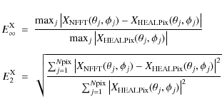
where X represents T, Q, U, or .

For field X is the maximum (relative) error, while is the relative root mean square error. Tables 1 and 2 provide the value of these statistics for unlensed CMB temperature only. Values of these error norms for the displacement field and the unlensed CMB polarization fields are of the same order of magnitude.

Table 1:   Variation in the typical orders of magnitude of error norms with the convolution length K for an unlensed CMB map simulated using NFFT.

Table 2:   Variation in the typical orders of magnitude of error norms with the oversampling factor for an unlensed CMB map simulated using NFFT.

To achieve this accuracy, we used the Kaiser-Bessel window (Kunis & Potts 2008; Fourmont 2003) as the NFFT interpolating function. Since the full precomputation of the window function at each node in spatial and frequency domains requires a large amount of memory space, we used a tensor product form for the multivariate window function, which requires only unidimensional precomputations. This method uses less memory at the price of some extra multiplications (Kunis & Potts 2008; Fourmont 2003). The accuracy (Kunis & Potts 2008; Fourmont 2003) of our simulation can be improved by increasing both the oversampling factor and the convolution length, at the price of extra memory consumption and CPU time (see Tables 1 and 2).

4.3 Simulation of lensed maps

We applied our simulation algorithm of lensed CMB maps (both temperature and polarization), described in Sect. 4.1, to 1000 independent realizations with HEALPix resolution , and a maximum multipole . In Fig. 2, we show one such realization of a lensed CMB temperature field, as well as the difference between the lensed and unlensed fields.

Since weak lensing of CMB is a tiny effect on small angular scales, we show a realization of a small portion of the unlensed CMB temperature anisotropies, lensed CMB temperature anisotropies, amplitude of deflection field and, the difference of lensed and unlensed CMB temperature anisotropies in Fig. 3 to illustrate the lensing effect more clearly. Although unlensed and lensed CMB temperature anisotropies are indistinguishable to the naked eye, the correlation between the deflection field and the difference between the lensed and unlensed CMB temperature anisotropies is clearly visible.

Table 3 shows the typical CPU time and memory required to simulate a single realization of unlensed and lensed CMB temperature and polarization, at different resolutions. These timings correspond to an AMD880 CPU running at 2.4 GHz. Storage of the window function at the grid points in both the spatial and frequency domain before computing the Fourier transform consumes a fair amount of memory, which ultimately increases the overall memory requirement for the simulation of lensed CMB maps (Kunis & Potts 2008; Fourmont 2003).

Table 3:   Variation in CPU time and memory requirements with resolution to simulate CMB maps (unlensed and lensed, oversampling factor , convolution length K=4) using NFFT.

Tables 4 and 5 show the same, but with varying convolution lengths and oversampling factors. Increase in the convolution length not only increases the computational cost of the interpolation part of NFFT, but also increases the cost of the precomputation of window function and memory requirement since one has to compute and store the window function at a larger number of grid points in the spatial domain before applying NFFT (Kunis & Potts 2008; Fourmont 2003). On the other hand, increasing the oversampling factor only impacts the memory and CPU requirements of the (oversampled) FFT part of the algorithm.

Table 4:   Variation in the CPU time and memory requirements with the convolution length K to simulate a CMB map (both unlensed and lensed, with nside = 1024, ) using NFFT.

Table 5:   Variation in CPU time and memory requirements with the oversampling factor for simulating a realization CMB map (both unlensed and lensed, nside = 1024, ) using NFFT.

On the same plots, Fig. 4 shows the theoretical power spectra C_l^XY, where XY represents TT,EE,TE and BB respectively, for the lensed and unlensed cases, as predicted by CAMB (Challinor & Lewis 2005). In the cosmological model, we decided to include no primordial tensors, hence C_l^BB is entirely due to lensing.

An accurate recovery of this power spectrum from lensed polarization maps is therefore a powerful test of our simulation method. In Fig. 5, we show, on top of the lensed theoretical spectra (lines), the average empirical power spectra computed from 1000 simulations (circles). We can see that the agreement is excellent, which is remarkable for C_l^BB as explained above. We have ignored the lensed angular power spectrum beyond the multipole l=1700 in the comparison, because the accurate computation of the average empirical power spectra for the multipoles l > 1700 requires lensed CMB maps simulated from the power spectra of unlensed CMB and a lensing potential beyond the multipole , which is the maximum multipole we used in the simulations. It is worth noting here that theoretical predictions for the B-mode power spectra induced from lensing, as computed in CAMB, are based on non-trivial, partially resummed expansions of correlation functions (Challinor & Lewis 2005). Figure 5 clearly shows very good agreement between the power spectra predicted from CAMB and measured from our simulations, therefore validating a posteriori the theoretical predictions.

To obtain a more quantitative view of the accuracy of the method, we show in Fig. 6 the relative difference between the average empirical power spectra computed on the 1000 simulations and the theoretical spectra from CAMB, both for the unlensed (red solid) and lensed (green dashed) cases. In each plot, we also show the theoretical root-mean-square deviation of the averaged empirical spectra, computed by neglecting the small lensing-induced non-Gaussianity in the lensed cases. Note that this corresponds to a very small underestimation of the scatter (Smith et al. 2006; Rocher et al. 2007). Taking into account that the averaged power spectra are nearly Gaussian distributed (due to the central limit theorem), we can assess the presence of possible biases in the recovered spectra by computing the reduced statistics:

here N_rlz is the number of independent realizations of angular power spectra under consideration.

Table 6:   Reduced statistics of the recovered unlensed angular power spectrum.

Table 7:   Reduced statistics for the recovered lensed angular power spectrum.

Tables 6 and 7 show that the probability of the reduced  statistics (Z²_XY)having values greater than their estimated values (z²_XY) is quite large for both unlensed and lensed power spectrum. This strengthens our claim about the unbiased nature of the simulation of unlensed and lensed CMB maps using NFFT.

5 Summary

Accurate predictions of the expected CMB anisotropies are required when analyzing future CMB data sets, which ultimately require accurately simulated lensed maps. The most popular pixelization used to analyze full-sky CMB maps is the HEALPix pixelization. To simulate lensed CMB anisotropies at HEALPix grid points, we must compute unlensed CMB anisotropies at irregularly spaced grid points over the sphere, determined by the deflection field and remapping equations. Since remapping on a sphere can be recast into remapping on a 2-d torus, we have used the NFFT library to compute lensed CMB anisotropies at HEALPix grid points and experimented with different settings of the accuracy parameters. We have found that for a nside = 1024 map a 10^-8 accuracy is easily reached when setting the parameters to (2,4). Our current implementation of the method consists of a 32 min computation on a classical PC configuration. This can probably be improved by parallelizing the algorithm (see Appendix D). Furthermore, the average angular power spectra recovered from 1000 realizations of lensed and unlensed CMB maps are also found to be consistent with the corresponding theoretical ones, . The agreement between our numerical power spectra estimates and the CAMB predictions is both a validation of our numerical method, and of the CAMB estimates based on partially resummed perturbative calculations.

These simulations will be a useful tool for the analysis and interpretation of upcoming CMB experiments such as Planck and ACT. However, they are not the only possible use of this technique. The simulation of the lensing deflection field can be improved by replacing the simple Born approximation with ray-tracing in dark matter N-nody simulations (Carbone et al. 2009,2008). Ray-tracing is affected by similar problems as the simulation of the lens effect on CMB maps, i.e., difficulties in accurately resampling a vector field on the sphere. Current state-of-the-art ray-tracing algorithms, such as (Teyssier et al. 2009), could be made more accurate by using the technique described here.

Appendix A: Spin s functions on a sphere and 2-d torus

Spin s square-integrable functions on a unit sphere are conveniently expanded in spin-weighted spherical harmonics of same spin (Goldberg et al. 1967; Newman & Penrose 1966; Zaldarriaga & Seljak 1997)

with the inverse transform,

These harmonics, with , and max , form an orthonormal basis for the decomposition of spin s square-integrable functions on the sphere. They are explicitly given in a factorized form in terms of the Wigner rotation matrices ,

With our assumed conventions for the Euler angles (Varshalovich et al. 1988; Edmonds 1957), we have,

These rotation matrices (A.4) basically characterize the rotation of spin-weighted spherical harmonics. The decomposition shown in Eq. (A.4) is exploited by factoring the rotation matrices into two separate rotation matrices as (McEwen et al. 2007; Wiaux et al. 2006),

Expressing the Wigner rotation matrices in Eq. (A.4) in the above manner of Eq. (A.5), Eq. (A.1) can be rewritten as

where

The advantage of writing the rotation matrices in this manner is that now the Euler angles only occur in complex exponentials and we only need to evaluate at (Varshalovich et al. 1988; Challinor et al. 2000; McEwen et al. 2007; Wandelt & Górski 2001; Risbo 1996; Edmonds 1957).

Computation of using Eq. (A.6) may not be the most efficient way, but the presence of exponentials may be exploited such that techniques of fast Fourier transform either on irregular or regular grid may be used for rapid computation of double summations simultaneously. In both cases, the domain of spin s function must be extended from the sphere, to the 2-dimensional torus, using the symmetry of spin-weighted spherical harmonics, so that Eq. (A.6) becomes a complex-to-complex Fourier transform over a 2-dimensional torus. The computation of _sf_{m  m'} for , involves performing a 1-dimensional summation over a 2-dimensional grid, hence it is of order .

Appendix B: Unlensed CMB fields on 2-d torus

Factoring the rotation matrices in two separate rotation matrices (A.4) and extending the domain of CMB, lensing potential and defection fields from sphere to 2-d torus, Eqs. (2), (3), (9), (10) can be rewritten as

and the corresponding Fourier modes are given by,

The extra factor of appears at the right-hand side of Eq. (B.8) because the deflection field is the gradient of the scalar potential field.

Appendix C: Lensed CMB fields on 2-d torus

Using the identities of the spherical triangle, lensed temperature anisotropies and polarization in a particular direction are given by unlensed temperature anisotropies and polarization in another direction at the last scattering surface.

The angular coordinates corresponding to the modified direction of the photon path due to lensing are determined by the deflection field ,

The extra factor , which appears in the case of the polarization (C.2), is there to rotate the basis vectors at to match them with the basis vectors at , such that

The Euler angles , and are defined as,

determines the angle between the directions and . The angle is that required to rotate the basis vector in a right-handed sense about onto the tangent (at ) to the geodesic connecting and , and is defined in the same manner as but at .

Appendix D: Parallelization of the algorithm

Significant speed improvements should be achieved by parallelizing the code. We review here the main parts of the code, and indicate possible ways of parallelizing them. We recall that the code is divided into two distinct parts. The first part computes the 2-d Fourier modes, starting from the spherical harmonic coefficients. This involves computing the Wigner coefficients , multiplying them with the spherical harmonic coefficients, and summing over the index. To reduce memory allocation, the summation over is computed on the fly in the outermost loop, together with the -recurrence of the Wigner coefficients. For each new , the (m,m') double recurrence is computed, its structure being local enough (using a modified version of the algorithm of Risbo 1996) for it to be parallelized at high  with small copies of boundary conditions. Another possibility would be to use the algorithm of Trapani & Navaza (2006), where the m recurrence is decoupled from the m'one, and can therefore be easily parallelized for each (see their Fig. 2).

The second is the FFT on irregular grid points, where we used the external library NFFT. Here the computation is divided into three parts: (i) precomputation of the window function around each real space node; (ii) diagonal correction of the Fourier modes and regular FFT; and (iii) discrete convolution for each node. Part (i) can be trivially parallelized since calculations are independent for each node. Part (ii) can also be easily parallelized using independent 1-d FFT calculation first along each line, and then along each column of the mode matrix (this scheme was already implemented into the FFTW library). Finally, part (iii) can also be parallelized by spatial domain decomposition of the nodes, with minor overlapping copies accounting for the support (K) of the truncated window. We note that in principle two different domain decompositions occur for the parallelization of the regular FFT and the parallelization of the operations on nodes (i.e., window function precomputation, discrete convolution). This could lead to important communication overheads and/or strong load imbalance in the case of very clustered nodes; in the case of weak lensing applications however, because of the small amplitude of the displacement field and the regularity of the HEALPix pixels, we do not expect this to be a major issue.

Acknowledgements

We acknowledge the use of the HEALPix package for our map pixelization. We also acknowledge the use of the NFFT package for our work. We thank Eric Hivon for helpful discussions and suggestions. One (SB) of the author's research at the Institut d'Astrophysique de Paris was supported by the Indo-French centre for promotion of advanced scientific research (CEFIPRA) through grant 3504-3. S.B. thanks Francois R. Bouchet and Tarun Souradeep for their constant encouragement and support throughout.

References

• Albrecht, A., & Steinhardt, P. J. 1982, Phys. Rev. Lett., 48, 1220 [NASA ADS] [CrossRef]
• Benabed, K., Bernardeau, F., & van Waerbeke, L. 2001, Phys. Rev. D, 63, 043501 [NASA ADS] [CrossRef]
• Blanchard, A., & Schneider, J. 1987, A&A, 184, 1 [NASA ADS]
• Carbone, C., Springel, V., Baccigalupi, C., Bartelmann, M., & Matarrese, S. 2008, MNRAS, 388, 1618 [NASA ADS] [CrossRef]
• Carbone, C., Baccigalupi, C., Bartelmann, M., Matarrese, S., & Springel, V. 2009, MNRAS, 576
• Challinor, A., Fosalba, P., Mortlock, D., et al. 2000, Phys. Rev. D, 62, 123002 [NASA ADS] [CrossRef]
• Challinor, A., & Lewis, A. 2005, Phys. Rev. D, 71, 103010 [NASA ADS] [CrossRef]
• Cooray, A., & Hu, W. 2001a, ApJ, 554, 56 [NASA ADS] [CrossRef]
• Cooray, A., & Hu, W. 2001b, ApJ, 548, 7 [NASA ADS] [CrossRef]
• Cooray, A., & Hu, W. 2002, ApJ, 574, 19 [NASA ADS] [CrossRef]
• Cooray, A., Hu, W., & Miralda-Escudé, J. 2000, ApJ, 535, L9 [NASA ADS] [CrossRef]
• Das, S., & Bode, P. 2008, ApJ, 682, 1 [NASA ADS] [CrossRef]
• Edmonds, A. R. 1957, Angular Momentum in Quantum Mechanics (Princeton, N.J.: Princeton University Press)
• Fourmont, K. 2003, Journal of Fourier Analysis and Applications, 9, 431 [CrossRef]
• Goldberg, J. N., Macfarlane, A. J., Newman, E. T., Rohrlich, F., & Sudarshan, E. C. G. 1967, Journal of Mathematical Physics, 8, 2155 [NASA ADS] [CrossRef]
• Górski, K. M., Hivon, E., Banday, A. J., et al. 2005, ApJ, 622, 759 [NASA ADS] [CrossRef]
• Guth, A. H. 1981, Phys. Rev. D, 23, 347 [NASA ADS] [CrossRef]
• Guzik, J., Seljak, U., & Zaldarriaga, M. 2000, Phys. Rev. D, 62, 043517 [NASA ADS] [CrossRef]
• Hirata, C. M., Padmanabhan, N., Seljak, U., Schlegel, D., & Brinkmann, J. 2004, Phys. Rev. D, 70, 103501 [NASA ADS] [CrossRef]
• Hirata, C. M., & Seljak, U. 2003a, Phys. Rev. D, 67, 043001 [NASA ADS] [CrossRef]
• Hirata, C. M., & Seljak, U. 2003b, Phys. Rev. D, 68, 083002 [NASA ADS] [CrossRef]
• Hu, W. 1999, ApJ, 522, L21 [NASA ADS] [CrossRef]
• Hu, W. 2000, Phys. Rev. D, 62, 043007 [NASA ADS] [CrossRef]
• Hu, W., & Tegmark, M. 1999, ApJ, 514, L65 [NASA ADS] [CrossRef]
• Hu, W., & Okamoto, T. 2002, ApJ, 574, 566 [NASA ADS] [CrossRef]
• Hu, W., & Okamoto, T. 2004, Phys. Rev. D, 69, 043004 [NASA ADS] [CrossRef]
• Kesden, M., Cooray, A., & Kamionkowski, M. 2002, Phys. Rev. D, 66, 083007 [NASA ADS] [CrossRef]
• Kesden, M., Cooray, A., & Kamionkowski, M. 2003, Phys. Rev. D, 67, 123507 [NASA ADS] [CrossRef]
• Kunis, S., & Potts, D. 2008, Sampling Theory in Signal and Image Processing, 7, 77
• Lesgourgues, J., Perotto, L., Pastor, S., & Piat, M. 2006, Phys. Rev. D, 73, 045021 [NASA ADS] [CrossRef]
• Lewis, A. 2005, Phys. Rev. D, 71, 083008 [NASA ADS] [CrossRef]
• Lewis, A., & Challinor, A. 2006, Phys. Rep., 429, 1 [NASA ADS] [CrossRef]
• Linde, A. D. 1982, Phys. Lett. B, 108, 389 [NASA ADS] [CrossRef]
• McEwen, J. D., Hobson, M. P., Mortlock, D. J., & Lasenby, A. N. 2007, IEEE Transactions on Signal Processing, 55, 520 [NASA ADS] [CrossRef]
• Newman, E. T., & Penrose, R. 1966, J. Math. Phys., 7, 863 [NASA ADS] [CrossRef]
• Okamoto, T., & Hu, W. 2003, Phys. Rev. D, 67, 083002 [NASA ADS] [CrossRef]
• Perotto, L., Lesgourgues, J., Hannestad, S., Tu, H., & Wong, Y. Y. 2006, J. Cosmol. Astro-Part. Phys., 10, 13 [NASA ADS] [CrossRef]
• Risbo, T. 1996, Journal of Geodesy, 70, 383 [NASA ADS]
• Rocher, J., Benabed, K., & Bouchet, F. R. 2007, J. Cosmol. Astro-Part. Phys., 5, 13 [NASA ADS] [CrossRef]
• Seljak, U. 1996, ApJ, 463, 1 [NASA ADS] [CrossRef]
• Smith, K. M., Hu, W., & Kaplinghat, M. 2006, Phys. Rev. D, 74, 123002 [NASA ADS] [CrossRef]
• Smith, K. M., Zahn, O., & Doré, O. 2007, Phys. Rev. D, 76, 043510 [NASA ADS] [CrossRef]
• Teyssier, R., Pires, S., Prunet, S., et al. 2009, A&A, 497, 335 [NASA ADS] [CrossRef] [EDP Sciences]
• Thorne, K. S. 1980, Rev. Mod. Phys., 52, 299 [NASA ADS] [CrossRef]
• Trapani, S., & Navaza, J. 2006, Acta Crystallographica A, 62, 262 [CrossRef]
• Van Waerbeke, L., Bernardeau, F., & Benabed, K. 2000, ApJ, 540, 14 [NASA ADS] [CrossRef]
• Varshalovich, D. A., Moskalev, A. N., & Khersonskii, V. K. 1988, Quantum Theory of Angular Momentum (Singapore: World Scientific Publishing Co.)
• Wandelt, B. D., & Górski, K. M. 2001, Phys. Rev. D, 63, 123002 [NASA ADS] [CrossRef]
• Wiaux, Y., Jacques, L., Vielva, P., & Vandergheynst, P. 2006, ApJ, 652, 820 [NASA ADS] [CrossRef]
• Zaldarriaga, M., & Seljak, U. 1997, Phys. Rev. D, 55, 1830 [NASA ADS] [CrossRef]
• Zaldarriaga, M., & Seljak, U. 1998, Phys. Rev. D, 58, 023003 [NASA ADS] [CrossRef]
• Zaldarriaga, M., & Seljak, U. 1999, Phys. Rev. D, 59, 123507 [NASA ADS] [CrossRef]

Footnotes

... code

http://cosmologist.info/lenspix

... points

http://www-user.tu-chemnitz.de/ potts/nfft

... FFT

http://www.fftw.org

... HEALPix

http://healpix.jpl.nasa.gov

... CAMB

http://camb.info

All Tables

Table 1:   Variation in the typical orders of magnitude of error norms with the convolution length K for an unlensed CMB map simulated using NFFT.

Table 2:   Variation in the typical orders of magnitude of error norms with the oversampling factor for an unlensed CMB map simulated using NFFT.

Table 3:   Variation in CPU time and memory requirements with resolution to simulate CMB maps (unlensed and lensed, oversampling factor , convolution length K=4) using NFFT.

Table 4:   Variation in the CPU time and memory requirements with the convolution length K to simulate a CMB map (both unlensed and lensed, with nside = 1024, ) using NFFT.

Table 5:   Variation in CPU time and memory requirements with the oversampling factor for simulating a realization CMB map (both unlensed and lensed, nside = 1024, ) using NFFT.

Table 6:   Reduced statistics of the recovered unlensed angular power spectrum.

Table 7:   Reduced statistics for the recovered lensed angular power spectrum.

All Figures

---

Copyright ESO 2009