| Issue |
A&A
Volume 508, Number 1, December II 2009
|
|
|---|---|---|
| Page(s) | 433 - 443 | |
| Section | The Sun | |
| DOI | https://doi.org/10.1051/0004-6361/200912664 | |
| Published online | 24 September 2009 | |
A&A 508, 433-443 (2009)
How skeletons turn into quasi-separatrix layers in source models
A. L. Restante1,2 - G. Aulanier1 - C. E. Parnell2
1 - LESIA, Observatoire de Paris, CNRS, UPMC, Université Paris Diderot,
5 place Jules Janssen, 92190 Meudon, France
2 - School of Mathematics and Statistics, University of St. Andrews,
St. Andrews, Fife KY16 9SS, Scotland, UK
Received 9 June 2009 / Accepted 17 September 2009
Abstract
Context. In situations where there are no magnetic
null points located above a reference photospheric plane, and when the
photospheric magnetic field is modeled by discrete flux concentrations,
the magnetic connectivity is defined by the magnetic skeleton of the
configuration. For a continuous distribution of non-zero photospheric
flux, the connectivity is defined by quasi-separatrix layers (QSLs).
Both the magnetic skeleton and QSLs can account for current sheet
formation and dissipation. Observationally, though, only some portions
of the skeleton are found to be related to flare ribbons, which are
generally associated with QSL footpoints.
Aims. In potential magnetic source models, a
transition from the skeleton to QSLs has been shown to occur when the
sources are displaced below the photospheric plane. The objective of
this paper is to understand the topological and geometrical nature of
this transition, and to derive rules to predict which parts of a given
skeleton will give rise to QSLs.
Methods. We consider magnetic configurations,
derived from potential magnetic sources, which possess no coronal null
points. We have calculated their skeletons, composed of null points,
spine field lines and separatrix (fan) surfaces. Choosing a reference
photospheric plane above the sources, we have calculated their QSL
footprints.
Results. As already known, the latter mostly match
with subphotospheric spine field lines since, above these lines, field
lines tend to diverge as a result of approaching a null and lying
either side of the separatrix surface extending out of from this null.
However, many non-spine related QSL footprints are also found, which we
call branches. They correspond to the intersection with the photosphere
of portions of fan field lines which ``branch'' away from the sources
and result in QSLs due to the inclination of the coronal field lines.
Conclusions. Our findings allow a better geometrical
understanding of the relations between QSLs and skeletons. We show that
in the absence of coronal null points, spines, as well as specific
portions of fans as calculated in standard potential source models, are
good predictors for the location of QSL footprints and of flare
ribbons.
Key words: Sun: magnetic fields
1 Introduction
Owing to its very low plasma resistivity and to its collisional nature, the low solar corona is a highly conductive medium which is governed by MHD. The powering of coronal heating in loops must therefore involve the formation of steep gradients of the magnetic field, namely current sheets, in initially smooth coronal magnetic fields. There is a wide variety of models that allow the development of such features, that have been reviewed and tested against some observational constraints by Démoulin et al. (2003). The first family of these models involve transient and alternative currents (AC), either created by MHD turbulence (e.g. Buchlin et al. 2003; Rappazzo et al. 2008; Gudiksen & Nordlund 2005) or by the resistive damping of nonlinear magnetoacoustic waves (e.g. Heyvaerts & Priest 1983; Ofman & Davila 1995; Einaudi & Mok 1987; Parker 1991). Such transient current sheets can develop in homogeneous distributions of the photospheric magnetic flux. The second family of models involve the formation of slowly amplifying direct currents (DC), which can naturally develop in driven line-tied magnetic fields. Such currents can form when the inhomogeneity of the photospheric magnetic field leads to the existence of discontinuities (or gradients) in the connectivity of magnetic field lines, along which current sheets spontaneously develop in a few Alfvèn times regardless of turbulence (e.g. Lau & Finn 1993; Low & Wolfson 1988; Haynes et al. 2007; Aly 1990; Aulanier et al. 2005). These DC coronal heating models are also commonly applied to the formation of reconnecting current sheets in solar flares (see the review of Démoulin 2007), which are very interesting events in which to study the relation between magnetic field connectivity, coronal reconnection, and observational signatures of energy deposition, since they occur on scales that involve much larger areas than those covered by each of the small energy release events that contribute to the heating of coronal loops.
In traditional DC models, the formation of a current sheet either involves the existence of a coronal magnetic null point, a bald patch, a separatrix surface or a separator line which connects two null points. In a potential magnetic field, the occurrence of a single coronal null point implies the presence of a closed inversion line for the vertical component of the photospheric magnetic field, all around a flux concentration whose sign is opposite to that of its neighbors (Aulanier et al. 2000; Antiochos 1998; Brown & Priest 2001). However, multiple coronal nulls can occur in more general potential magnetic fields. The occurrence of a bald patch implies the existence of portions of inversion lines along which field lines are tangent to the photosphere, and across which the horizontal field is directed from the negative to the positive polarity (Titov et al. 1993). Even though observed solar flaring events have been clearly associated to coronal null points (Ugarte-Urra et al. 2007; Aulanier et al. 2000; Masson et al. 2009) and to bald patches (Mandrini et al. 2002; Pariat et al. 2004; Aulanier et al. 1998) as calculated from force-free field extrapolations, it has been shown that these situations do not account for the majority of energetic events at active region scales (Démoulin 2007; Démoulin et al. 1994b).
The occurrence of null points, in particular photospheric null points, and coronal separators, is a very natural property of magnetic field configurations which are formed by discrete photospheric flux concentrations (either singular or extended), around which there is no magnetic flux passing through the photosphere (e.g. Longcope & Klapper 2002; Priest et al. 2005; Close et al. 2005; Démoulin et al. 1994a; Gorbachev & Somov 1989; Maclean et al. 2009; Schrijver & Title 2002). Such models can therefore result in a complex distribution of distinct flux domains, whose boundaries are defined by separatrix fan surfaces. These fans form part of the skeleton of the magnetic field, when combined with their associated photospheric null points and spine field lines (Longcope 1996). Such models have been applied to observations of bright points (e.g. Longcope 2001; Maclean et al. 2009; Parnell et al. 1994) and flares (Des Jardins et al. 2009; Barnes et al. 2005; Longcope et al. 2005,2007). In general, however, the use of discrete sources and the magnetic skeleton has been applied to try and determine not only the number and approximate position of the reconnection sites, but also to determine the energy released during reconnection. This is because, with the magnetic skeleton, it is very easy to determine the amount of flux transferred between flux domains and hence estimates can be made of the currents generated and then released during these flux changes. In particular, this is the philosophy that led to the development of the minimum current corona model (Longcope 1996; Longcope & Cowley 1996; Longcope 2001), which has been used to model flares to determine where and how much energy is released (e.g. Barnes et al. 2005; Longcope & Silva 1998; Longcope et al. 2007). Furthermore, Priest et al. (2002) have applied the magnetic skeleton approach to create a coronal model to explain coronal heating. Close et al. (2004,2005) considered quiet-Sun magnetograms and, using the magnetic skeleton approach, were able to determine that during solar minimum all the magnetic connections within the corona are replaced in just 1.4 h, a factor of 10 times faster than the recycling time of the magnetic features in the quiet-Sun photosphere (Hagenaar 2001). When applied to flare observations, clear correlations have been found between the locations of observed chromospheric bright ribbons and of the low altitude trace of the modeled skeletons (e.g. Des Jardins et al. 2009; Longcope & Beveridge 2007; Démoulin et al. 1994a; Longcope et al. 2007).
In reality, though the Sun's surface is not composed of large regions where the normal component of the magnetic field to the surface is zero. This means that, on the Sun itself, there will be far fewer nulls lying exactly on the surface, and hence far fewer genuine separators that are anchored at the Sun's surface. Thus, an alternative approach, avoiding these unnatural zero normal field regions, is commonly used in which complex photospheric magnetic fields are modeled in terms of a continuous distribution of flux. Here, the connectivity of the magnetic field is no longer defined by its skeleton, but rather by quasi-separatrix layers (QSLs), which are narrow volumes across which the mapping of the magnetic field displays strong gradients (Démoulin et al. 1996a; Priest & Démoulin 1995). The connectivity gradients can then be quantified by the squashing degree of the flux tubes (Titov 2007; Titov et al. 2002). Very thin QSLs, characterized by very large squashing degrees, are natural regions for reconnecting current sheets to develop, as a result of any line-tied footpoint motion (Aulanier et al. 2006,2005). The formation and dissipation of current sheets in quiet-Sun like magnetic field configurations have therefore been proposed to account for coronal heating (Aulanier et al. 2005; Démoulin & Priest 1997), just like in skeleton models. Also, QSLs have been found to fully match observed flare ribbons (e.g. Démoulin et al. 1996a,1997; Bagalá et al. 2000; Mandrini et al. 1996; Schmieder et al. 1997), in contrast to the magnetic skeleton which only partially are associated with the ribbons.
The narrowest QSLs therefore generalize the concept of separatrices, in non-idealized magnetic field configurations. Bridging the gap between separatrices and QSLs has been the object of several studies. First, the highest squashing degrees are found within hyperbolic flux tubes (HFTs) and so these features can be thought of as the ``core'' of a QSL. A separator (which is at the intersection of two separatrix surfaces) appears to be similar to an infinitely squashed HFT (Démoulin et al. 1996a; Titov et al. 2002, 2003; Galsgaard et al. 2003) and the HFT footprints were noted to be located above spine field lines by Titov et al. (2002). Second, in a given magnetic field configuration built from magnetic sources, it has been shown that a transition, from the skeleton to QSLs, takes place when all the sources and related null-points are displaced from the photospheric layer to below it (Démoulin et al. 1996a; Titov & Hornig 2002). The dependence of the maximum value of the squashing degree, with respect to the depth of the sources, has there been found to be a power law, the index of which depends on the relative positioning of the sources. Also, the closer the sources are placed to the photospheric plane, the greater the portions of the skeleton that are covered by the QSL footprints. Third, these findings have recently been complemented by the spatial correlation found between QSL footprints and parallel electric fields integrated along reconnecting field lines in an MHD simulation that used a potential field extrapolations as initial conditions, with parts of the complex skeletons that were calculated in various discrete flux concentration models for the same observed photospheric magnetic field (Maclean et al. 2009).
Our interest is in the associations between QSLs, magnetic skeletons and flare ribbons. So in this paper, we further pursue the analysis of the link between skeletons and QSLs. We show and explain geometrically which parts of the skeleton of any given magnetic field configuration, built with magnetic sources, can turn into QSLs. Our results therefore can be used to predict which elements of the magnetic field, in source models, can be involved in coronal reconnection, and where flare ribbons can be located in the chromosphere. We use potential field models to conduct this study, therefore our results only apply to magnetic field configurations which overall connectivity that can be approximated by potential field extrapolations. So we do not address the issue of the geometrical nature of QSLs in regions that are very non-potential on global scales, such as those resulting from wide twisted flux tubes (as in e.g. Démoulin et al. 1996b; Titov & Démoulin 1999, in which bald patch bifurcations play a major role).
2 Four sources
2.1 Studied configurations
We analyze the topology and the field line linkage where a potential
magnetic field is created from point sources, i.e. monopoles. In such
source models, in Cartesian geometry, (x,y,z)
where the sources are placed on a ![]() plane and so z refers to the altitude or depth and
the magnetic field
plane and so z refers to the altitude or depth and
the magnetic field ![]() is singular at the sources. Away from the sources, it is given by:
is singular at the sources. Away from the sources, it is given by:
| Bx(x,y,z) | = | 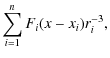
|
(1) |
| By(x,y,z) | = | 
|
(2) |
| Bz(x,y,z) | = | 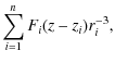
|
(3) |
| ri | = | (4) |
where n is the number of sources, Fi is the flux of the sources and (xi,yi,zi) are the positions of the sources.
Potential fields are interesting to conduct our study for several reasons. Historically, they have been used to calculate coronal topologies relating them to flares and other coronal phenomena, amongst other uses (see Sect. 1). It has been found that this approximation (including the linear force-free one) is often sufficient to model small confined flares and bright points. Physically, it is expected that the overall topology of a quasi force-free (non dynamic) magnetic field configuration should not be very sensitive to non-potential effects if the electric currents are distributed on a scale which is smaller than that of one of the bipoles. Indeed, Aulanier et al. (2005) and Pariat et al. (2009) show that relatively small-scale currents do not change their overall QSL and null-point topology, respectively, whereas Haynes et al. (2007) found the formation of new separators in dynamically moving bipoles embedded in horizontal fields, and Démoulin et al. (1996b) and Titov & Démoulin (1999) showed how large-scale twisted fields induce new QSLs and bald patches, respectively. The present study therefore does not apply to non force-free fields and/or to force-free fields that contain strong and large-scale currents.
We initially consider two configurations which have already
been investigated in the literature by Démoulin
et al. (1996a, hereafter D96) and Aulanier et al. (2005, hereafter A05).
We chose these configurations for three main reasons. First, their QSLs
have been calculated in the related papers. D96 actually calculated the
QSLs using the norm N (see Eq. (5)) at various
altitudes above that of the sources, which brought first insights to
the transition between QSLs and magnetic skeleton structures. Second,
because the features of these two configurations are similar. They are
both formed by four sources, which define a smaller bipole of weak flux
embedded in a main larger bipole of stronger flux. In particular, in
D96 at z = 0 the smaller bipole has weaker magnetic
fields than the larger one, whereas in A05, due to the different depth
of the sources
which form the larger bipole, the magnetic fields of the smaller bipole
are stronger than that of the larger bipole. Both configurations have
the same main bipole, with its axis along x. In
D96, the inner bipole is roughly parallel to the axis of the main
bipole (both bipoles make an angle ![]() ), whereas
the bipoles are nearly antiparallel in A05 (
), whereas
the bipoles are nearly antiparallel in A05 (
![]() ). Third, A05 is different to
most continuous source models, because its two bipoles are placed at
different depths, which creates an asymmetry in the model, as well as
spine field lines which are inclined in altitude. Table 1 summarizes the
parameters of the sources in both configurations.
). Third, A05 is different to
most continuous source models, because its two bipoles are placed at
different depths, which creates an asymmetry in the model, as well as
spine field lines which are inclined in altitude. Table 1 summarizes the
parameters of the sources in both configurations.
Table 1: Parameters of the magnetic configurations with 4 sources.
![\begin{figure}
\par\includegraphics[width=12cm,clip]{12664fig1.eps}
\vspace*{2mm}
\end{figure}](/articles/aa/full_html/2009/46/aa12664-09/img15.png)
|
Figure 1:
Magnetic field topology and geometry for the D96 model; a)
displays a map of the squashing degree Q(x,y,z=0)
that shows QSL footprints at z=0, above the
altitude of the sources. White stands for |
| Open with DEXTER | |
2.2 Photospheric footprints of quasi-separatrix layers
Here we briefly recall what quasi-separatrix layers (QSLs) are, and how
to calculate them. QSLs are regions where there is a rapid change in
field line
linkage (Démoulin
et al. 1996a; Priest & Démoulin 1995).
In other words, these regions correspond to large mapping distortions
or strong ``squashing'' of flux tubes (Titov
et al. 2002). QSLs can be calculated by measuring
the squashing degree Q. Let us consider, in the
Cartesian geometry, the field line mapping from one footpoint at a
given layer z0 to
the other at the same layer:
![]() and the
reverse one. These mappings can be represented by some vector
functions
[X-
(x+ , y+),
Y- (x+
, y+)] and [X+
(x- , y-),
Y+ (x-
, y-)], respectively. From
these,
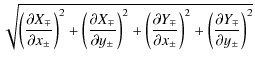
for the determination of QSLs, Priest
& Démoulin (1995)
proposed to use the functions N(r+)
and N(r-)
(called ``the Norm'' because they represent the norm
of the respective Jacobian Matrices):
and the
reverse one. These mappings can be represented by some vector
functions
[X-
(x+ , y+),
Y- (x+
, y+)] and [X+
(x- , y-),
Y+ (x-
, y-)], respectively. From
these,
for the determination of QSLs, Priest
& Démoulin (1995)
proposed to use the functions N(r+)
and N(r-)
(called ``the Norm'' because they represent the norm
of the respective Jacobian Matrices):
It was proposed that
When different normal field components (Bz+
and
Bz-) exist
in the field line footpoints, a difficulty with the
definition of QSLs by
Eq. (5)
is that ![]() if
if ![]() .
To overcome this, Titov et al.
(2002) defined another characteristic function for QSLs which
is
independent of the mapping direction: the squashing degree Q.
It is
calculated as follows:
.
To overcome this, Titov et al.
(2002) defined another characteristic function for QSLs which
is
independent of the mapping direction: the squashing degree Q.
It is
calculated as follows:
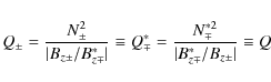
where the functions that have asterisks indicates that their arguments x- and y- are substituted in X- (x+ , y+), and Y- (x+ , y+) respectively. With this prescription a QSL is defined by
![\begin{figure}
\par\includegraphics[width=12cm,clip]{12664fig2.eps}
\vspace*{3mm}
\end{figure}](/articles/aa/full_html/2009/46/aa12664-09/img27.png)
|
Figure 2: Magnetic field topology and geometry for the A05 model. The drawing conventions are the same as in Fig. 1. |
| Open with DEXTER | |
Hereafter, the z=0 plane will be referred to the
``photosphere'', by analogy with past studies in which subphotospheric
sources were considered to emulate the observed distribution of the
magnetic field in the solar photosphere. So as to compute the
photospheric QSL footprints in our two magnetic configurations, the QSL
formulas (Eq. (6))
have been coupled with the MPOLE![]() libraries, which integrate field lines. The coordinates of the
endpoints of the field lines are extracted from MPOLE, since they are
required to calculate Q from Eq. (6). We used a uniform
grid in both x and y directions
with a grid spacing of
libraries, which integrate field lines. The coordinates of the
endpoints of the field lines are extracted from MPOLE, since they are
required to calculate Q from Eq. (6). We used a uniform
grid in both x and y directions
with a grid spacing of ![]() ,
which is comparable to that used by D96 and A05. The resulting maps of Q(z=0)
are plotted in Figs. 1a
and 2a
in a domain
,
which is comparable to that used by D96 and A05. The resulting maps of Q(z=0)
are plotted in Figs. 1a
and 2a
in a domain ![]() and
and ![]() .
.
The calculated QSLs have the same shapes and localization as reported in D96 and A05. In the D96 configuration, they form two roughly parallel ``lanes'' of Q and the maximum of Q, at z = 0, is approximately located where the norm of the magnetic field is minimum. Each lane ends in two little curved hooks. In A05, the shape of the QSLs is different to that in D96. Even though the maxima of Q are still located around the magnetic field minimum regions, the QSL footprints are arc-shaped and each arc points toward the middle of the other. From this finding, one could first state that the QSLs are always located around minimum magnetic field areas. But this is not sufficient to understand their shape, and their direction of elongation.
2.3 Fan and spine separatrices emanating from the sources
Instead of using MPOLE to calculate and plot the nulls, the fans and the spines in our four-source models, we use the so-called sources method (SM, see Démoulin et al. 1994b,a), which we briefly describe below.
Firstly, in order to find and to characterize null points, the
magnetic field is discretized on a mesh. The sign of the 3 magnetic
field components is then calculated on the 12 edges of each 3D cell.
When the three components of the field are found to reverse at least
once along any of the edges of a cell, a Newton-Raphson method is
applied to locate precisely the position of the null in three
dimensions. The eigenvectors of the null are then calculated using the
standard null-point formulas (see e.g. Parnell et al. 1996; Lau & Finn 1990):
| B | = | (7) | |
| M | = | 
|
(8) |
In our configurations, the three eigenvalues of M are real and two nulls Nu1 and Nu2 are present, and are located in between two sources of the same polarity, as in Molodenskii & Syrovatskii (1977). In D96, the nulls lie on the same plane as that of the sources, i.e. at z=-0.1, and are all prone nulls, whereas, in A05, the nulls are located at an intermediate altitude between the sources which are situated at different depths.
Secondly, for each of the nulls, we integrate with a predictor-corrector scheme the spines in both directions following the eigenvector associated with the eigenvalue whose sign is opposite to that of the other two. In D96 the resulting spines have Bz=0 and are exactly located in the horizontal plane of the sources, whereas they have finite and varying Bz values in A05. We use the two other eigenvectors to integrate a set of fan field lines. As found by Fukao et al. (1975), in our case, as in all potential fields, the fan plane is perpendicular to the spine.
The nulls, spines and fans are plotted in Figs. 1 and 2 for the D96 and A05 configurations, respectively. The calculated separatrices are of the same type as those found before in four-source models involving two pairs of opposite polarity sources (e.g. Gorbachev & Somov 1989; Greene 1988): the spines are low-lying and the fans take the shape of domes which intersect at high altitude along a separator line that connects both nulls.
2.4 Relation between spines and QSL footprints
Comparing Figs. 1a and 2a with Figs. 1b and 2b one readily sees that not only the largest photospheric Q areas are located close to the positions of the sub-photospheric null-points, but also that the main orientation of the QSL footprints roughly follows that of the sub-photospheric spines. This relation was noticed first by Titov et al. (2002). The QSL footprints then tend to join two sources of the same polarity, following a path along which Bz(z=0) does not changes its sign (i.e. not crossing photospheric inversion lines), and with decreasing Q values as one moves away from the null-points.
Independently of Titov et al. (2002), parts of the spines of real prone nulls have recently been hinted to be associated with QSLs in potential field source models. First, Des Jardins et al. (2009) found that parts of such spines were located close to regions of Hard X-ray footpoint emission as observed by RHESSI on top EUV ribbons which developed during three eruptive flares. Since flare ribbons have also been found to match very well with QSL footprints in several case studies (e.g. Démoulin 2007; Démoulin et al. 1997; Mandrini et al. 1996; Bagalá et al. 2000; Schmieder et al. 1997), their results are similar to ours, even though the applicability of potential fields as models for eruptive flares is questionable. Second Maclean et al. (2009) compared a set of source models with several MHD simulations of an observed bright point. They found that some parts of their calculated skeleton (mostly including spines, and also some fans when looking at their figures) roughly matched both the footprints of the strongest regions of the parallel electric field integrated along the field lines and that of the QSLs, both calculated by Büchner (2006).
Still, these previous results have not fully addressed the question of the nature of the transition between elements of the magnetic skeleton and QSLs, and have not addressed the details of the association of spine field lines to QSL footprints. Indeed, Maclean et al. (2009) write ``the obvious question remaining is, why does only part of the separatrix surface correspond to the location of the strong integrated parallel electric field and the QSL?''.
Our results clearly show that, when the number of sources is relatively small, the topological transition from the magnetic skeleton to QSLs, which occurs when the nulls pass below the reference photospheric plane, leads to a transformation of the field lines near the nulls that run close to the spine into photospheric QSL footprints. Titov et al. (2002) wrote about the latter that ``these are the separatrix lines approaching the nulls perpendicular to the fan surfaces''. This transition can be geometrically explained as follows. If one considers a set of field lines whose starting points are placed in a vertical half-circle of infinitesimal radius that surrounds a nearly horizontal sub-photospheric spine, the field lines will eventually diverge from one another when they approach the null point, and then, they will simply graze the fan surface at large altitudes above the plane of the sources. This same behavior will occur further and further from the null point, but with less divergence, as one increases the radius of the circle of the field line starting points. All this is a natural property of a potential null-point geometry. This explains why the photospheric maximum of Q is always located close to the position of the sub-photospheric null-point, the shift only being a natural consequence of the bending of the field lines in response to the flux of the sources. Moreover, by construction, when the reference photospheric plane is placed slightly (resp. far) above the null-point locations, the diverging pattern of the field lines above that plane will be strong (resp. weak), so this explains why the QSL footprints are more (resp. less) extended with stronger (resp. weaker) maximum Q values, as seen on the plots and the measurements of the N quantity in D96.
Consequently, a first estimator of a QSL footprint, i.e. a first estimator of the location of flare ribbons and of HXR emissions during reconnection in the solar corona in relatively simple geometries, can simply be given by the distribution of prone nulls and spines in source models.
Still, Figs. 1 and 2 show that the lower Q extremities of the QSL footprints, namely the hooks in D96 and the arcs in A05, not only pass the location of the sources, but are also much longer than the spines. D96 also clearly showed that, when the depth of the sources is very close to that of the photosphere at which the QSLs are calculated, the QSL footprint eventually covers the intersection of the separatrix surfaces with the photosphere as well. This shows right away that simply associating QSL footprints and spines is only an approximation. Understanding the full nature of the transition between the magnetic skeleton and QSLs therefore requires further investigation. Since it is not straightforward to understand this with our four source models, we address this issue hereafter with a multiple source model.
3 Multi sources
Table 2: Parameters of the magnetic configuration with 15 sources.
![\begin{figure}
\par\includegraphics[width=15cm,clip]{12664fig3.eps}
\vspace*{4mm}
\end{figure}](/articles/aa/full_html/2009/46/aa12664-09/img33.png)
|
Figure 3:
Magnetic field topology and geometry for the model with 15 sources;
a) displays a map of the squashing degree Q(x,y,z=0)
that shows QSL footprints at z=0, above the
altitude of the sources. The sources are indicated by + (resp. |
| Open with DEXTER | |
3.1 Strong spine-related QSLs in complex configurations
In this section, we consider a more complex geometry than before. We
consider
an asymmetric distribution made of 15 balanced sources with different
intensities. The source parameters are given in Table 2. We consider a set
of balanced sources to avoid the presence of artificial sources away
from the selected field of view with (
![]() ). We chose all sources at the
same level z = -0.1 on a square grid with 361
points in each direction in x and y.
We selected the source parameters in order to have all the nulls lying
on the same plane as that of the sources and selected the sources in
such away as to
avoid the occurrence of any upright nulls. Thus, all the spines lie in
the same plane z=-0.1 and there are no vertical
spines associated with upright nulls or high altitude null points (as
in e.g. Aulanier
et al. 2000; Antiochos 1998; Brown &
Priest 2001; Pariat
et al. 2009). The latter would lead to nulls, spines
and separatrix surfaces which would be structurally stable (e.g. not
turn into QSLs) provided the photospheric plane was not chosen to be
above them, as it inevitably is for the surface nulls.
). We chose all sources at the
same level z = -0.1 on a square grid with 361
points in each direction in x and y.
We selected the source parameters in order to have all the nulls lying
on the same plane as that of the sources and selected the sources in
such away as to
avoid the occurrence of any upright nulls. Thus, all the spines lie in
the same plane z=-0.1 and there are no vertical
spines associated with upright nulls or high altitude null points (as
in e.g. Aulanier
et al. 2000; Antiochos 1998; Brown &
Priest 2001; Pariat
et al. 2009). The latter would lead to nulls, spines
and separatrix surfaces which would be structurally stable (e.g. not
turn into QSLs) provided the photospheric plane was not chosen to be
above them, as it inevitably is for the surface nulls.
So as to calculate QSLs footprints (shown in Fig. 3a), we used the same method as described in Sect. 2.2. To calculate null points and separatrices, we use both the MPOLE and the SM, as described earlier. MPOLE finds null points using a combination of reasonable initial guesses, and it iterates from them until it finds the locations of the nulls (Longcope 1996). Both methods gave the same 13 surface nulls, from which we calculated the related skeleton, as plotted in Figs. 3b, d.
The resulting skeleton and QSL footprints have a much more complex pattern than in the 4 source models. This enables us to analyze several situations, so as to determine more general rules which govern the topological transitions from the magnetic skeleton to QSLs.
One can see that the strong relation found before between spines and QSL footprints remains valid. Most of the QSL footprints (where Q takes the higher values) still lie above the spines. Moreover, this configuration reveals that, when two consecutive spines follow each other through a given source, there having a sharp discontinuity in their directions, a continuous corresponding QSL footprint is found above the spines, and it displays a smooth curvature around the position of the source. This behavior is sketched in Fig. 4a. This situation is found to be very common in our configuration, e.g. between the sources P1-3-4, P4-6-8. Such consecutive spine patterns were also found in the source models of Des Jardins et al. (2009). This transition which we find now clearly explains the relation between several consecutive spines modeled in various source models by Maclean et al. (2009) and the overlying smoother distribution of the footprints of QSLs and of the electric field integrated along the field lines, calculated by Büchner (2006) in a full MHD simulation.
3.2 Identification of non-spine related QSLs
There are number of regions where the QSL footprints are actually not related to spines. The QSL pattern shown in Fig. 3a indeed has more structure than shown by the spines alone in Fig. 3b. Three types of non-spine related QSL footpoints can be identified: due to of their shapes, we will refer to them as ``branches''.
The first significant branches (see Fig. 3a) are the two very long QSL footprints (b1, b2) which emanate, respectively, from the sources P1 and P2. They cross the positive polarities at z=0, as if they were a simple extension of the QSL footprint associated with spines lying in the z=-0.1 between P1-3 and P2-5, respectively. The branches extend from the positive sources toward the null points located below on z=-0.1 between N1-2 and N1-5 respectively, but they do not reach them. Instead, they end close to the curved part of the inversion line that closes around the related positive flux concentration at z=0. Interestingly, a major difference between these QSL footprints and those associated with spines is that, for the former, Q peaks at a maximum close to a magnetic source, whereas for the latter Q is maximum near the null-point. Unlike in the 4 source models, those branches cannot be regarded as minor, because of their relatively large lengths. Also, these are clearly not an artifact of our calculation. Indeed, the U-shape of the inversion lines naturally imply shell-shapes for the distribution of field lines located above z=0. In other words, the field lines form a set of arcades above the inversion line, which have the shape of a curve tunnel. At the base of this shell pattern, a gradient of connectivity is naturally expected (as found in magnetic field extrapolations by Mandrini et al. 1996; Schmieder et al. 1997, for an observed bright point and a C-class flare, respectively).
| Figure 4: Three main behavior of Q factor around sources (+): a) shows when we have two consecutive spines (S), the QSLs footprint fallow their shape, but tend to smooth the point connection between them; b) shows Q factor follows the spine shape (S) until it has a fan contribution (F) that is given by the end points of fan field lines starting from the source (+) on the photospheric plane. In this case it curves on that shape; c) shows that b) case is true, but when we have also the presence of a consecutive spine, the Q factor smoothly follow it and also branch on following the fans contribution. |
|
| Open with DEXTER | |
| Figure 5:
Toy model for understand the nature of the branches:
a) in blue we report the fan field lines, in
red (in orange) a couple of field line starting from a distance |
|
| Open with DEXTER | |
A second type of long branch is rooted in the source P8 (e.g. V in Fig. 3a). It has a V-shape. So it is actually composed of two QSLs, which not only merge with one another in a flux concentration, but which also merge with another QSL, that one being associated to the consecutive spines P6-8-7. As found above, Q in these branches decreases away from the magnetic source, oppositely to what is found in spine-related QSLs. This V-shape QSL pattern is also not an artifact of the calculations, since field line plots show that these two QSLs separate the positive flux concentration at z=0, that results from the P8 source, in three quasi connectivity domains, which are linked to the negative flux concentrations associated with N2-1-5.
The third type of branch consists of many small curved QSL footprints (e.g. a1, a2, c1, c2 in Fig. 3a), which are located close to almost all other spine-related QSLs. They typically display low Q values, and they have arc shapes. Some of them have horse-shoe shapes, they graze the spines and partly surround sources (e.g. around N3 (c1) and N4 (c2)). Such QSL footprints have already been reported in Mandrini et al. (1996) and Schmieder et al. (1997). Other arc shaped branches in our model have weaker curvatures, and they simply extend away from the sources (e.g. near N2 (a1) and between N6-7 (a2)). Because of their lengths and shapes, these seem to be of the same kind as the small hook and arc-shaped QSL extensions which we identified in the 4 source models.
3.3 The role of fan field lines
QSLs have already been found in simple bipolar configurations, in which the corresponding potential fields calculated from point- or line-sources would not possess null points, and therefore no spines. But this has only been reported in highly non-potential fields, in which large-scale shear or twist either creates an S shape bald patch separatrix (Titov & Démoulin 1999) or a double-J shape QSL footprint pattern (Titov 2007; Démoulin et al. 1996b). But in potential source models, one can hardly imagine how QSLs could not be related to any topological property of the potential magnetic field configuration.
Apart from the spine field lines, the only topological elements in source models are the separatrix (or fan) surfaces. Fan field lines calculated with the SM are plotted in Fig. 3d. Note that for most of the fans, we have not plotted field lines covering their whole surface. This is visible, for example in Fig. 3d, for the red fan associated with the null point between N1-3, for the dark-blue fan associated with the null point between P4-6, and for two very large-scale red and green fans associated with the null points between N1-2 and N1-5 respectively. The reason is that for most of the null points, the fans are far from being axisymmetric around the axis of the spine, because the complex distribution of sources results in generating fan-related eigenvectors of different amplitudes. For the 4 nulls described above, the ratio between the pair of fan eigenvalues of each null is 3.5, 4.9, 8.1 and 24, respectively. In these cases, fan field lines starting from the null bend in directions parallel or anti-parallel to the eigenvector associated with the largest eigenvalue, as described by Parnell et al. (1996) and found by Mandrini et al. (2006) for photospheric null points and by Masson et al. (2009) for coronal (i.e. high altitude) null points.
The sum of spines and fans (Fig. 3d) now show more structures than the QSL footprints (Fig. 3a). Still, one can surprisingly associate the V shape and the spine extension branches, with the two red and green fans of very large eigenvalue ratios described above. Those match very well with one another. This fan-branch relation was not expected from the results from our 4 source models, and then could not be predicted with our first explanation of QSL footprint locations on plane above point sources. However, this relation is far from being obvious elsewhere in the model. This shows that, in general, only a subset of the fan field lines can transform into QSL footprints.
On one hand, there is not a single branch that starts from the null points, even though Q there peaks to large values. On the other hand, only the parts of fans that start from the sources seem relate to branches. To clarify this, we plotted in Fig. 3c the spines at z=-0.1 as well as the portions of fan field lines only, starting from the sources at z=-0.1 and ending in the photospheric plane at z=0 (where Q was calculated). Comparing this with Fig. 3a, one can see that these photospheric ending points all match with the branches. As can be seen, for example, with the fuchsia fan portions that start from the sources P3-4-6, whose photospheric endpoints fit the horse-shoe shape branch that surrounds the source N4. A similar association can be seen around N7, where the spine-related QSL footprint does not end in the source, but rather splits into different branches that correspond to the endpoints of the blue, cyan and green fan field lines. The topological transitions from separatrices to QSLs in these two examples are sketched in Figs. 4b, c. This finding explains the reason why the long V shape and spine extension branches were readily matched by the drawn red and green fan field lines. Indeed, the very small relative amplitude of the z-aligned fan eigenvector in these two fans permits a very small amount of magnetic flux to cross the z=0 plane. So the majority of field lines which we plotted in Fig. 3d were actually confined below z=0.
The full curve that joins the photospheric endpoints of field lines which belong to a given fan, and which start from a given source, extend from close to this source at z=0 up to the inversion line at z=0. If this whole curve would turn into a QSL footprint in all cases, then all branches should stop just before an inversion line. Figure 3a shows that this indeed happens (see e.g. the long branches which link the spine-related QSL footprints from P1, P2 and P7), but that it is not the case in general (see e.g. the branches which emanate from N2 and N7). These different behaviors actually relate to the lower limit for Q(z=0) for which one considers a QSL to be significantly narrow (i.e. important).
So, qualitatively, our results show that apart from the main spine-related QSL footprints, QSL branches correspond to the curve defined by the photospheric endpoints of all fan field lines which start from a subphotospheric source. This gives us an improved estimator for QSL footprints in source models.
3.4 Comparison with the 4 source models and interpretation
If one reconsiders the previous simple models which we addressed in this paper in light of the above findings, one can now relate the hook and arc shape QSL footprints to the branches in the complex 15 source model. Figures 1 and 2 indeed show an excellent match between the low-Q extensions of the QSLs with the ends at z=0 of the thick portions of the subphotospheric fan field lines originating from the sources.
As for the transformation of subphotospheric spines into QSL footprints, the topological transition between fan field lines and QSL branches can be understood from the geometry of field lines. Two field lines starting from a subphotospheric source (e.g. P1 in D96) on both sides of a given fan remain roughly parallel along the fan, with weakly varying distances between one another across the fan (which is formed by red lines in Fig. 1b). Close to the null point (Nu2 in Fig. 1b) however, these same field lines actually diverge from one another as they tend to follow the spine (S2 in Fig. 1d) in opposite directions (towards N1 and N2). As a consequence, the photospheric trace of these field lines, close to the initial source (P1), is smaller than that close to the null point (Nu2). This implies the presence of a relatively strong squashing degree Q, hence a branch, around the photospheric trace of the fan close to the source. This explains the fan contribution to the QSL footprints.
One can go further and explain the reason why Q decreases away from the source in these branches. Consider, in a first approximation, that the eigenvectors of the fan have comparable amplitudes, so that the null point structure can be considered to be axisymmetric around the spine axis. In order to have this configuration, we can for example generate a minimized model (Fig. 5) using three balanced sources (two of them being positive) placed along the same line at the same altitude. In this geometry we have only one null having both fan eigenvectors with the same eigenvalue. This implies that in this case we have a radial symmetric fan which simplifies the analysis of the field line geometries. As in our other models, the sources are placed on a plane below the plane taken as the photosphere.
Consider two pairs of field lines, which start from the negative source (N1) and lie either side of the fan surface, which comes from the null point (Nu1) and let each pair be located around a different fan field line: one of them leaving the null at right angles to the plane of sources, and the other inclined at an acute angle to this plane (still allowing the surrounding field lines to pass above the photospheric plane). The two pairs of field lines, drawn in orange and red in Fig. 5a, are chosen so as to result in equal distances between their photospheric footpoints above N1. Their subphotospheric portions are drawn in black, so as to visualize their intersections with the photospheric plane. When both pairs reach the photosphere close to the null point, they both diverge along the spine that joins the P1 and P2 sources. In particular, the red pair of field lines diverge there more than the orange pair: the footpoint distance of the orange lines at the vicinity of the null point is smaller than that of the red lines. This implies that on the footprints of the fan field line surrounded by the red pair (resp. the orange pair), close to (resp. far from) the position of the source, the Q-factor is higher (resp. lower). This fits the QSL footprint which we calculated in this configuration, as shown in Fig. 5b.
In order to explain this behavior and to apply this finding in the general case, we further analyze the way different pairs of field lines intersect a photospheric plane placed above that of the sources. In Fig. 5, the red and the orange field lines were selected so that the horizontal distance between their pairs of photospheric footpoints at the vicinity of the negative source was equal. Due to the symmetry of the configuration, each pair with its middle fan field line lies on the same plane, the one for the red pair being vertical and the one for the orange pair being inclined. For the analysis, let us rotate the plane of the orange lines vertically, so that all field lines now belong to the same plane. Doing this, we keep the length of initial subphotospheric field line segments, drawn in black in Fig. 5a. The resulting 2D field line distribution is plotted in Fig. 5c. In this projection, the altitude of the photosphere is larger in the orange lines than in the red lines, due to the applied rotation of the plane of the orange lines. Due to the axisymmetric properties of this configuration, this projection readily results in one (blue) fan field line, closely surrounded by the pair of orange lines, themselves being surrounded by the red lines, all along their length. Close to the null point, all field lines that are close to the fan tend to diverge away from it, so as to follow the spine toward the sources P1 and P2. Therefore, for both pairs of field lines, their separation from the fan is smaller (resp. larger) at larger (resp. smaller) altitudes above the null point Nu1. So, in the 2D projection, the distance between the orange lines, at the (higher) altitude of their own photosphere, must be smaller than their distance at the (lower) altitude of the photosphere of the red lines, which is in turn smaller than the distance between the red lines. These geometrical properties show that the ratio between the photospheric footpoints above Nu1 and above N1 for the orange lines is smaller than that for the red lines. Hence, the Q-factor for the red lines must be larger, and must decrease away from the source toward the orange lines.
In other words, the orange pair of field lines, which originate in the z=0 plane further from the sources, actually lie closer together across the separatrix surface than the red pair. Hence, they remain closer (to the separatrix surface) all the time they are above the photosphere and only diverge as they are near the null below the photosphere. Hence, they have a lower Q.
This explains why, contrary to spine-related QSL footprints, fan-related branches display lower and lower Q further and further away from the sources.
3.5 Connections between branches and null-halos
In Fig. 5b one can see that the QSLs footprint is formed by two distinct patterns. The one located around the source N1 is formed by the branches, and the other one is located around the null point Nu1. The latter consists of a high-Q core due to the contribution of the underlying spine that connects P1 and P2, as well as a low-Q halo centered around the null point, which we refer to as the ``null-halo'' hereafter.
Following the orange pair of field lines in Fig. 5a, we see that the footpoints that correspond to the ends of the branches are linked with footpoints on the edge of the null-halo which extends perpendicularly to the underlying spine direction. If we consider Figs. 1a, c and 2a, c we find the same behavior. As shown in Figs. 1c and 2c, if we take starting footpoints along a segment that crosses the QSL footprint above the underlying null and perpendicular to its spine direction (pink Q1 from a cut across Nu1 and green Q2 from a cut across Nu2 ), one notices that their conjugate footpoints lie all along the conjugate QSL footprint. The high Q, centre of the perpendicular cut, corresponds to the spine of the conjugate QSL's null, and the low Q halo corresponds to the branches of the conjugate QSL footprint region.
As we have already mentioned, Q is constant along the field lines. Within the null-halo, the field lines rooted in the region that is far from the spine are therefore connected to the branches, whereas those rooted closer to and over the spine are connected to the conjugate spine-related QSL footprint. So the length of the branches seem to be directly related to the width of their related null-halo, in the direction perpendicular to the underlying spine. This is also valid in the more complicated case Fig. 3: comparing the different panels, one can relate each branch with its conjugate null-halo. For example, consider the branches V rooted in the source P8 and their associated parts b1 and b2 (see Fig. 3a). They are connected to the null-halo around the null points located between the sources N1-N2 and N1-N5, respectively. Also, the upper branch of a1 and the left branch of a2 are connected to the conjugate null-halo between P6-P8. Such associations can be found for each fan shown in Fig. 3d, by relating them to branches and null-halos in Fig. 3a. All these associations, if we consider the limitations due to the presence of other spine contributions and polarity inversion lines (PILs), suggest that the length of the branches seems to be related to the width of the conjugate null-halo.
It is noteworthy that, in general, the longer the branches (i.e. the more they cover the fan projection on the photospheric plane) the narrower the QSL footprint (as shown by Démoulin et al. 1996a; and in Sect. 2.4) and the larger the maximum value of Q (or N). Indeed in our models, when one compares the QSLs footprints in the D96 and A05 configurations (Figs. 1, 2a), short (resp. long) branches that cover little (resp. almost all) of the fan projection up to the PILs are found. This is related to the fact that in D96 (resp. in A05), there are relatively small (resp. large) values of Q (as clearly seen in the divergence of the colored Q1 and Q2 field lines in Figs. 1c and 2c), hence to a relatively wider (resp. narrower) width of the spine-related QSL footprint. Since the length of the branches is related to the width of the null-halo, we find the interesting and counter-intuitive result that the narrower the core of the QSL footprint, the wider its null-halo.
4 Conclusion
In this paper, we investigated the topological transition between
magnetic skeleton and QSL footprints. Our study was motivated by the
fact that, despite there being a good relation between the magnetic
skeleton and QSLs, so far this relation is not well understood. The QSL
footprints match only a part of the skeleton projected on the
photospheric plane (where one can calculate the squashing degree, i.e.
the Q-factor) (Démoulin et al. 1996a; Maclean
et al. 2009), but the precise relation between them
has not yet been investigated. Understanding this relation is important
because flare ribbons as observed in H![]() as well as in hard X-rays have been shown to match well with QSL
footprints (Démoulin et al. 1996a,
1997), whereas the ribbons match only part of the skeleton (Des Jardins
et al. 2009; Démoulin et al. 1994b; Longcope
et al. 2007).
Moreover, even if the regions of strong Q-factor
localize better the ribbons, and give a good prediction where current
sheets can form when the system is perturbed, the magnetic skeleton is
easier to calculate. Indeed, it only requires the location of magnetic
null points to be found. This may explain why magnetic skeleton
calculations are, as of today, more widely used than QSL calculations.
as well as in hard X-rays have been shown to match well with QSL
footprints (Démoulin et al. 1996a,
1997), whereas the ribbons match only part of the skeleton (Des Jardins
et al. 2009; Démoulin et al. 1994b; Longcope
et al. 2007).
Moreover, even if the regions of strong Q-factor
localize better the ribbons, and give a good prediction where current
sheets can form when the system is perturbed, the magnetic skeleton is
easier to calculate. Indeed, it only requires the location of magnetic
null points to be found. This may explain why magnetic skeleton
calculations are, as of today, more widely used than QSL calculations.
Our goal was two fold. First, we aimed to quantify the topological relation between the topology and the quasi-topology with geometrical arguments. Second, we wanted to find a general method for predicting which parts of the skeleton, calculated with source models, turn into QSL footprints when the photosphere is considered to be located above all magnetic sources, so as to predict the location of current sheets and flare ribbons, in non-eruptive configurations.
We considered three different magnetic field configurations: two relatively simple ones with four sources, already considered in previous studies (Démoulin et al. 1996a; Aulanier et al. 2005) which we refer to in this paper as D96 and A05, respectively, and a more complex one formed by an asymmetric set of 15 sources. In all these models, we calculated the QSL photospheric footprints (the photospheric regions that have the strongest squashing degree), by placing the photosphere at some small altitude above that of the sources, and we compared these regions with all the components of the calculated skeleton (null points, fan surfaces, spine field lines).
In the D96 configuration (see Fig. 1), we noticed that the maxima of Q, the squashing factor, were located near (above) the position of the nulls, and that the shape of the sheet-like distribution formed by the strongest Q values tends to follow the shape of the spine, but not all of it. This is fully consistent with the plots of N in D96. When we considered the A05 geometry (Fig. 2), we found that the QSL footprint was more elongated than the spine projected on the photosphere. In order to understand non-spine related parts of QSL footprints, we investigated a more complex geometry (Fig. 3), generated by 15 sources located at the same subphotospheric height and chosen such that all the null points were in the same plane as the sources. In this configuration, as in the two previous ones, we found many parts of the QSLs footprint (which we called ``branches'') that were not due to spine contributions. We found the interesting result that all branches actually follow the first intersection with the photosphere of the fan's field lines starting from subphotospheric sources.
We explained that the topological transition between spines and QSL footprints can be attributed to the divergence of field lines from the spines. Consider, for instance, a positive null from which a separator extends to a negative null. When two field lines lying close to the spine from the positive null, but on different sides of the separatrix surface from the negative null (and vice versa) they cause a large Q-factor on their foot prints. We also managed to explain the origin of the branches (i.e. non-spine related QSL footprints) as being due to the spreading of field lines (along a spine field line) being located on either side of a fan surface and originating from a flux concentration, a spreading which we explained to be less and less important for pairs of field lines anchored further and further from the flux concentration. Since the Q-factor is constant along field lines, we also explained why some isolated spines (i.e. not related to a separator) can result in a QSL footprint.
With these findings, any one using source and skeleton models should be able to identify which parts of complex skeletons can be related to QSL footprints and (non-eruptive) flare ribbons, by applying the following rules:
- The maxima of the Q-factor in the photosphere are located near and above the position of the subphotospheric null points.
- The shape of the maximum values of the Q-factor tend to follow the spine shape (as first noticed by Titov et al. 2002), but not all of it.
- The non-spine related QSL footprints (i.e. branches) match with the curves defined by the photospheric endpoints of all fan field lines that start from subphotospheric sources and their conjugate footprints which are rooted in the related null-halo.
We thank the referee for his/her comments which helped to improve this paper and we also thank P. Démoulin and T. Török for their helpful discussions. We also acknowledge the financial support by the European Commission through the SOLAIRE network (MTRM-CT-2006-035484).
References
- Aly, J. J. 1990, Publ. Debrecen Heliophys. Obs., 7, 176
- Antiochos, S. K. 1998, ApJ, 502, L181 [NASA ADS] [CrossRef]
- Aulanier, G., Démoulin, P., Schmieder, B., Fang, C., & Tang, Y. H. 1998, Sol. Phys., 183, 369 [NASA ADS] [CrossRef]
- Aulanier, G., DeLuca, E. E., Antiochos, S. K., McMullen, R. A., & Golub, L. 2000, ApJ, 540, 1126 [NASA ADS] [CrossRef]
- Aulanier, G., Pariat, E., & Démoulin, P. 2005, A&A, 444, 961 [NASA ADS] [CrossRef] [EDP Sciences]
- Aulanier, G., Pariat, E., Démoulin, P., & Devore, C. R. 2006, Sol. Phys., 238, 347 [NASA ADS] [CrossRef]
- Bagalá, L. G., Mandrini, C. H., Rovira, M. G., & Démoulin, P. 2000, A&A, 363, 779 [NASA ADS]
- Barnes, G., Longcope, D. W., & Leka, K. D. 2005, ApJ, 629, 561 [NASA ADS] [CrossRef]
- Brown, D. S., & Priest, E. R. 2001, A&A, 367, 339 [NASA ADS] [CrossRef] [EDP Sciences]
- Buchlin, E., Aletti, V., Galtier, S., et al. 2003, A&A, 406, 1061 [NASA ADS] [CrossRef] [EDP Sciences]
- Büchner, J. 2006, Space Sci. Rev., 122, 149 [NASA ADS] [CrossRef]
- Close, R. M., Parnell, C. E., & Priest, E. R. 2004, Sol. Phys., 225, 21 [NASA ADS] [CrossRef]
- Close, R. M., Parnell, C. E., & Priest, E. R. 2005, Geophys. Astrophys. Fluid Dyn., 99, 513 [NASA ADS] [CrossRef]
- Démoulin, P. 2007, Adv. Space Res., 39, 1367 [NASA ADS] [CrossRef]
- Démoulin, P., & Priest, E. R. 1997, Sol. Phys., 175, 123 [NASA ADS] [CrossRef]
- Démoulin, P., Henoux, J. C., & Mandrini, C. H. 1994a, A&A, 285, 1023 [NASA ADS]
- Démoulin, P., Mandrini, C. H., Rovira, M. G., Henoux, J. C., & Machado, M. E. 1994b, Sol. Phys., 150, 221 [NASA ADS] [CrossRef]
- Démoulin, P., Henoux, J., Priest, E., & Mandrini, C. 1996a, A&A, 308, 643 [NASA ADS]
- Démoulin, P., Priest, E. R., & Lonie, D. P. 1996b, J. Geophys. Res., 101, 7631 [NASA ADS] [CrossRef]
- Démoulin, P., Bagala, L. G., Mandrini, C. H., Henoux, J. C., & Rovira, M. G. 1997, A&A, 325, 305 [NASA ADS]
- Démoulin, P., van Driel-Gesztelyi, L., Mandrini, C. H., Klimchuk, J. A., & Harra, L. 2003, ApJ, 586, 592 [NASA ADS] [CrossRef]
- Des Jardins, A., Canfield, R., Longcope, D., Fordyce, C., & Waitukaitis, S. 2009, Sol. Phys.
- Einaudi, G., & Mok, Y. 1987, ApJ, 319, 520 [NASA ADS] [CrossRef]
- Fukao, S., Ugai, M., & Tsuda, T. 1975, Report Ionosphere Space Research Japan, 29, 133 [NASA ADS]
- Galsgaard, K., Titov, V. S., & Neukirch, T. 2003, ApJ, 595, 506 [NASA ADS] [CrossRef]
- Gorbachev, V. S., & Somov, B. V. 1989, SvA, 33, 57 [NASA ADS]
- Greene, J. 1988, J. Geophys. Res., 93, 8583 [NASA ADS] [CrossRef]
- Gudiksen, B. V., & Nordlund, Å. 2005, ApJ, 618, 1020 [NASA ADS] [CrossRef]
- Hagenaar, H. J. 2001, ApJ, 555, 448 [NASA ADS] [CrossRef]
- Haynes, A. L., Parnell, C. E., Galsgaard, K., & Priest, E. R. 2007, Royal Society of London Proc. Ser. A, 463, 1097 [NASA ADS] [CrossRef]
- Heyvaerts, J., & Priest, E. R. 1983, A&A, 117, 220 [NASA ADS]
- Lau, Y.-T., & Finn, J. 1990, ApJ, 350, 672 [NASA ADS] [CrossRef]
- Lau, Y.-T., & Finn, J. M. 1993, Phys. Fluids B, 5, 365 [NASA ADS] [CrossRef]
- Longcope, D. 2001, Phys. Plasmas, 8, 5277 [NASA ADS] [CrossRef]
- Longcope, D. W. 1996, Sol. Phys., 169, 91 [NASA ADS] [CrossRef]
- Longcope, D. W., & Beveridge, C. 2007, ApJ, 669, 621 [NASA ADS] [CrossRef]
- Longcope, D. W., & Cowley, S. C. 1996, Phys. Plasmas, 3, 2885 [NASA ADS] [CrossRef]
- Longcope, D., & Klapper, I. 2002, ApJ, 579, 468 [NASA ADS] [CrossRef]
- Longcope, D. W., & Silva, A. V. R. 1998, Sol. Phys., 179, 349 [NASA ADS] [CrossRef]
- Longcope, D. W., McKenzie, D. E., Cirtain, J., & Scott, J. 2005, ApJ, 630, 596 [NASA ADS] [CrossRef]
- Longcope, D., Beveridge, C., Qiu, J., et al. 2007, Sol. Phys., 244, 45 [NASA ADS] [CrossRef]
- Low, B. C., & Wolfson, R. 1988, ApJ, 324, 574 [NASA ADS] [CrossRef]
- Maclean, R. C., Büchner, J., & Priest, E. R. 2009, A&A, 501, 321 [NASA ADS] [CrossRef] [EDP Sciences]
- Mandrini, C. H., Démoulin, P., van Driel-Gesztelyi, L., et al. 1996, Sol. Phys., 168, 115 [NASA ADS] [CrossRef]
- Mandrini, C. H., Démoulin, P., Schmieder, B., Deng, Y. Y., & Rudawy, P. 2002, A&A, 391, 317 [NASA ADS] [CrossRef] [EDP Sciences]
- Mandrini, C. H., Demoulin, P., Schmieder, B., et al. 2006, Sol. Phys., 238, 293 [NASA ADS] [CrossRef]
- Masson, S., Pariat, E., Aulanier, G., & Schrijver, C. J. 2009, ApJ, 700, 559 [NASA ADS] [CrossRef]
- Milano, L. J., Gomez, D. O., & Martens, P. C. H. 1997, ApJ, 490, 442 [NASA ADS] [CrossRef]
- Milano, L. J., Dmitruk, P., Mandrini, C. H., Gómez, D. O., & Démoulin, P. 1999, ApJ, 521, 889 [NASA ADS] [CrossRef]
- Molodenskii, M. M., & Syrovatskii, S. I. 1977, SvA, 21, 734 [NASA ADS]
- Ofman, L., & Davila, J. M. 1995, J. Geophys. Res., 100, 23413 [NASA ADS] [CrossRef]
- Pariat, E., Aulanier, G., Schmieder, B., et al. 2004, ApJ, 614, 1099 [NASA ADS] [CrossRef]
- Pariat, E., Antiochos, S. K., & DeVore, C. R. 2009, ApJ, 691, 61 [NASA ADS] [CrossRef]
- Parker, E. N. 1991, ApJ, 372, 719 [NASA ADS] [CrossRef]
- Parnell, C. E., Priest, E. R., & Golub, L. 1994, Sol. Phys., 151, 57 [NASA ADS] [CrossRef]
- Parnell, C., Smith, J., Neukirch, T., & Priest, E. 1996, Phys. Plasmas, 3, 759 [NASA ADS] [CrossRef]
- Priest, E., & Démoulin, P. 1995, J. Geophys. Res., 100, 23 [CrossRef], 443
- Priest, E. R., Heyvaerts, J. F., & Title, A. M. 2002, ApJ, 576, 533 [NASA ADS] [CrossRef]
- Priest, E. R., Longcope, D. W., & Heyvaerts, J. 2005, ApJ, 624, 1057 [NASA ADS] [CrossRef]
- Rappazzo, A. F., Velli, M., Einaudi, G., & Dahlburg, R. B. 2008, ApJ, 677, 1348 [NASA ADS] [CrossRef]
- Schmieder, B., Aulanier, G., Demoulin, P., et al. 1997, A&A, 325, 1213 [NASA ADS]
- Schrijver, C., & Title, A. 2002, Sol. Phys., 207, 223 [NASA ADS] [CrossRef]
- Titov, V. S. 2007, ApJ, 660, 863 [NASA ADS] [CrossRef]
- Titov, V. S., & Démoulin, P. 1999, A&A, 351, 707 [NASA ADS]
- Titov, V. S., & Hornig, G. 2002, Adv. Space Res., 29, 1087 [NASA ADS] [CrossRef]
- Titov, V. S., Priest, E. R., & Demoulin, P. 1993, A&A, 276, 564 [NASA ADS]
- Titov, V., Hornig, G., & Démoulin, P. 2002, J. Geophys. Res., 107, 3 [CrossRef]
- Titov, V. S., Galsgaard, K., & Neukirch, T. 2003, ApJ, 582, 1172 [NASA ADS] [CrossRef]
- Ugarte-Urra, I., Warren, H. P., & Winebarger, A. R. 2007, ApJ, 662, 1293 [NASA ADS] [CrossRef]
Footnotes
- ... MPOLE
![[*]](/icons/foot_motif.png)
- MPOLE 2.4, http://solar.physics.montana.edu/dana/mpole/mpole_doc.html
All Tables
Table 1: Parameters of the magnetic configurations with 4 sources.
Table 2: Parameters of the magnetic configuration with 15 sources.
All Figures
|
|
Figure 1:
Magnetic field topology and geometry for the D96 model; a)
displays a map of the squashing degree Q(x,y,z=0)
that shows QSL footprints at z=0, above the
altitude of the sources. White stands for |
| Open with DEXTER | |
| In the text | |
|
|
Figure 2: Magnetic field topology and geometry for the A05 model. The drawing conventions are the same as in Fig. 1. |
| Open with DEXTER | |
| In the text | |
|
|
Figure 3:
Magnetic field topology and geometry for the model with 15 sources;
a) displays a map of the squashing degree Q(x,y,z=0)
that shows QSL footprints at z=0, above the
altitude of the sources. The sources are indicated by + (resp. |
| Open with DEXTER | |
| In the text | |
| |
Figure 4: Three main behavior of Q factor around sources (+): a) shows when we have two consecutive spines (S), the QSLs footprint fallow their shape, but tend to smooth the point connection between them; b) shows Q factor follows the spine shape (S) until it has a fan contribution (F) that is given by the end points of fan field lines starting from the source (+) on the photospheric plane. In this case it curves on that shape; c) shows that b) case is true, but when we have also the presence of a consecutive spine, the Q factor smoothly follow it and also branch on following the fans contribution. |
| Open with DEXTER | |
| In the text | |
| |
Figure 5:
Toy model for understand the nature of the branches:
a) in blue we report the fan field lines, in
red (in orange) a couple of field line starting from a distance |
| Open with DEXTER | |
| In the text | |
Copyright ESO 2009
Current usage metrics show cumulative count of Article Views (full-text article views including HTML views, PDF and ePub downloads, according to the available data) and Abstracts Views on Vision4Press platform.
Data correspond to usage on the plateform after 2015. The current usage metrics is available 48-96 hours after online publication and is updated daily on week days.
Initial download of the metrics may take a while.