Gravitational lenses as cosmic rulers: , from time delays and velocity dispersions

D. Paraficz; J. Hjorth

doi:10.1051/0004-6361/200913307

Home

All issues

Volume 507 / No 3 (December I 2009)

A&A, 507 3 (2009) L49-L52

Full HTML

Free Access

Issue		A&A Volume 507, Number 3, December I 2009


Page(s)		L49 - L52
Section		Letters
DOI		https://doi.org/10.1051/0004-6361/200913307
Published online		04 November 2009

A&A 507, L49-L52 (2009)

LETTER TO THE EDITOR

Gravitational lenses as cosmic rulers: ${\Omega_{\rm m}}$ , $\Omega _{\Lambda }$ from time delays and velocity dispersions

D. Paraficz - J. Hjorth

Dark Cosmology Centre, Niels Bohr Institute, University of Copenhagen, Juliane Maries Vej 30, 2100 Copenhagen, Denmark

Received 16 September 2009 / Accepted 28 October 2009

Abstract
We show that a cosmic standard ruler can be constructed from the joint measurement of the time delay, $\Delta \tau$ , between gravitationally lensed quasar images and the velocity dispersion, $\sigma$ , of the lensing galaxy. This is specifically shown, for a singular isothermal sphere lens, $D_{\rm OL} \propto \Delta \tau / \sigma^2$ , where $D_{\rm OL}$ is the angular diameter distance to the lens. Using MCMC simulations we illustrate the constraints set in the $\Omega_{\rm m}-\Omega_{\Lambda}$ plane from future observations.

Key words: gravitational lensing - Galaxy: kinematics and dynamics - cosmology: theory - cosmology: dark matter

1 Introduction

In the cosmological $\Lambda$ CDM model, it is currently estimated that 96% of the total energy density of the Universe is in the form of dark matter (25%) and dark energy (74%). These proportions have been inferred from a number of completely independent measurements, e.g. cosmic microwave background (CMB) (Spergel et al. 2003; Komatsu et al. 2009), baryon acoustic oscillations (Eisenstein et al. 2005), supernovae (Riess et al. 1998; Perlmutter et al. 1999), large scale structure (Peacock et al. 2001), clusters of galaxies (White et al. 1993) and weak gravitational lensing (Weinberg & Kamionkowski 2003). Unfortunately, any astrophysical approach suffers from potential systematic uncertainties (e.g. supernovae - not standard but standardized candles with possible redshift evolution; CMB - various parameter degeneracies and interference with foregrounds; weak lensing - PSF influencing the galaxy shape measurement). It is therefore important to explore complementary methods for measuring these quantities. Gravitationally lensed quasars QSOs offer such an attractive alternative.

QSOs that are positioned in a way that a lens, i.e., a massive foreground object such as a galaxy or a group of galaxies, intersects the line of sight, can be seen as magnified, multiple images. Gravitationally lensed QSOs have already been used to set constraints on cosmological parameters. Notably Refsdal (1964) showed that the Hubble constant H₀ can be measured from a multiple imaged QSO if the time delay between the lensed images and the mass distribution of the lens are known; attempts to constrain the cosmological constant $\Lambda$ have been based on gravitationally lensed QSO statistics (Fukugita et al. 1990). The importance of strong gravitational lensing in future constraints on the evolution of the dark energy equation of state parameter w(z), has also been emphasized (Linder 2004).

In recent years, joint studies of stellar dynamics and gravitational lensing have proven very fruitful, e.g. the Lenses Structure & Dynamics (LSD) Survey and the Sloan Lens ACS Survey (SLACS) were used to constrain the density profiles of galaxies (Koopmans et al. 2006; Treu & Koopmans 2004). Methods for using either velocity dispersions (Grillo et al. 2008) or time delays (Dobke et al. 2009) of lensed systems have been proposed as estimators of ${\Omega_{\rm m}}$ and $\Omega _{\Lambda }$ .

We note that a standard cosmic ruler can be constructed from the joint measurement of the time delay between QSO images and the velocity dispersion of the lensing galaxy, independent of the redshift of the QSO. We explore its use to constrain ${\Omega_{\rm m}}$ and $\Omega _{\Lambda }$ in view of the large samples of lenses to be found in forthcoming experiments, such as from the Large Synoptic Survey Telescope (LSST), Square Kilometre Array (SKA), Joint Dark Energy Mission (JDEM), Euclid, and the Observatory for Multi-Epoch Gravitational Lens Astrophysics (OMEGA) (Marshall et al. 2005; Moustakas et al. 2008; Ivezic et al. 2008; Carilli & Rawlings 2004; Dobke et al. 2009).

2 Lenses as standard rulers

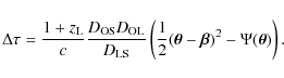
The time delay $\Delta \tau$ is the combined effect of the difference in length of the optical path between two images and the gravitational time dilation of two light rays passing through different parts of the lens potential well,

$\begin{displaymath}% \Delta\tau = \frac{1+z_{\rm L}}{c}\frac{D_{\rm OS}D_{\rm OL... ...1}{2} (\vec{\theta}-\vec{\beta})^2-\Psi(\vec{\theta})\right). \end{displaymath}$

(1)

Here $\vec{\theta}$ and $\vec{\beta}$ are the positions of the images and the source respectively, $z_{\rm L}$ is the lens redshift, and $\Psi$ is the effective gravitational potential of the lens. $D_{\rm OL}$ , $D_{\rm OS}$ , $D_{\rm LS}$ are the angular diameter distances between observer and lens, observer and source, and lens and source, respectively. If the lens geometry $\vec{\theta} - \vec{\beta}$ and the lens potential $\Psi$ are known, the time delay measures the ratio $D_{\rm OS}D_{\rm OL}/D_{\rm LS}$ , also known as the effective lensing distance $r(z,\Omega_{\rm m},\Omega_\Lambda)$ , which depends on the cosmological parameters.

The observed velocity dispersion of a galaxy $\sigma$ is the result of the superposition of many individual stellar spectra, each of which has been Doppler shifted because of the random stellar motions within the galaxy. Therefore, it can be determined by analyzing the integrated spectrum of the galaxy, which has broadened absorption lines due to the motion of the stars. The velocity dispersion is related to the mass through the virial theorem: $\sigma^2\propto M_{\sigma}/R$ , where $M_{\sigma}$ is the mass enclosed inside the radius R. The mass is measured by the Einstein angle $\theta_{\rm E}$ of the lensing system $M_{\theta_{\rm E}}=\frac{c^2}{4G} \frac{D_{\rm OL}D_{\rm OS}}{D_{\rm LS}}\theta_{\rm E}^2$ , where $R=D_{\rm OL}\theta_{\rm E}$ . Thus, $\sigma^2 \propto \frac{D_{\rm OS}}{D_{\rm LS}}\theta_{\rm E}$ .

Since the time delay is proportional to $D_{\rm OS}D_{\rm OL}/D_{\rm LS}$ and the velocity dispersion is proportional to $D_{\rm OS}/D_{\rm LS}$ , the ratio $\Delta \tau /\sigma ^2$ is dependent only on the lens distance and therefore acts as a cosmic ruler: $\Delta\tau/\sigma^2 \propto D_{\rm OL}$ . In Fig. 1 we illustrate the dependency on the lens redshift of the measurables, time delay $\Delta \tau$ , velocity dispersion squared $\sigma ^2$ , and the ratio between them, $\Delta \tau /\sigma ^2$ . To show the sensitivity of the three functions to $\Omega _{\Lambda }$ , we plot them for four cases of a flat ( $\Omega _{\rm m}+\Omega _{\Lambda }=1$ ) Universe with $\Omega _{\Lambda }$ = 0.2, 0.5, 0.7 and 0.9, relative to an Einstein-de Sitter Universe ( $\Omega_{\rm m}=1, \Omega_{\Lambda}=0$ ).

We can see that $\Delta \tau /\sigma ^2$ is more sensitive to the cosmological parameters than $\Delta \tau$ or $\sigma ^2$ separately. We also note that the higher the lens redshift, the more pronounced is the dependency on cosmology, hence it is important for this method to study high redshift lenses. Finally, it has the advantage of being independent of the source redshift.

$\begin{figure} \par\includegraphics[width=6.8cm,clip]{13307fg1.ps} \end{figure}$

Figure 1:

Dependence of the three quantities, $\Delta \tau$ ( top panel), $\sigma ^2$ ( middle panel), $\Delta \tau /\sigma ^2$ ( bottom panel) on the lens redshift. The source redshift was fixed to z=3. A flat Universe ( $\Omega _{\rm m}+\Omega _{\Lambda }=1$ ) was assumed with 4 different values $\Omega _{\Lambda }$ : 0.2, 0.5, 0.7 and 0.9. Each curve is plotted relative to a flat Einstein-de Sitter Universe ( $\Omega _{\rm m}=1$ , $\Omega _{\Lambda }=0$ ).

Open with DEXTER

Both velocity dispersion and time delay depend on the gravitational potential of the lens galaxy. For the simple case of a singular isothermal sphere (SIS) both parameters can be easily expressed analytically. While the SIS model is convenient for its simplicity, it is also a surprisingly useful model for lens galaxies (Koopmans et al. 2006; Guimarães & Sodré 2009; Koopmans et al. 2009; Schechter & Wambsganss 2004; Oguri 2007).

The time delay is

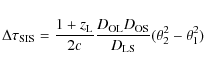
$\begin{displaymath}% \Delta\tau_{\rm SIS} = \frac{1+z_{\rm L}}{2c} \frac{D_{\rm OL}D_{\rm OS}}{D_{\rm LS}}(\theta_2^2-\theta_1^2) \end{displaymath}$

(2)

and the velocity dispersion is

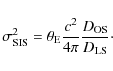
$\begin{displaymath}% \sigma^2_{\rm SIS} = \theta_{\rm E}\frac{c^2}{4\pi}\frac{D_{\rm OS}}{D_{\rm LS}}\cdot \end{displaymath}$

(3)

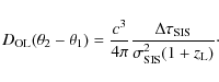
For the SIS model the Einstein angle is half the distance between the lensed images, $\theta_{\rm E}=(\theta_1+\theta_2)/2$ (we define $\Delta \tau$ and $\theta_{1,2}$ to be positive, with $\theta_2 \ge \theta_1$ ). Hence

$\begin{displaymath}% D_{\rm OL} (\theta_2-\theta_1) = \frac{c^3}{4\pi} \frac{\Delta\tau_{\rm SIS}} {\sigma^2_{\rm SIS}(1+z_{\rm L})}\cdot \end{displaymath}$

(4)

3 Monte Carlo Markov Chain simulations

To explore the constraints set on cosmological parameters from the joint measurements of image positions, lens redshift, time delay and velocity dispersion, we perform simulations on SIS lenses using the Metropolis algorithm (Saha & Williams 1994). To simulate the uncertainties of the measurables we use $\chi^2$ given by:

$\begin{displaymath}% \chi^2= \frac{ \left[\frac{\Delta\tau}{\sigma^2\theta_{\rm... ...\tau}{\sigma^2\theta_{\rm E}(1+z_{\rm L})}\right)^2 \right]}, \end{displaymath}$

(5)

where, for simplicity we have assumed that for each simulated lens, the lens images are aligned such that $\theta_1=0$ and $\theta_2=2\theta_{\rm E}$ . Similar expressions are computed for $\Delta \tau$ and $\sigma ^2$ . In all the simulations we let $\Omega_{\rm m},\Omega_\Lambda$ vary between 0 to 1 while either fixing or marginalizing over H₀.

$\begin{figure} \par\includegraphics[width=6.8cm,clip]{13307fg2.ps} \end{figure}$

Figure 2:

MCMC simulations for three different cases: $\Delta \tau$ ( top, panel), $\sigma ^2$ ( middle panel), and $\Delta \tau /\sigma ^2$ ( bottom panel). 125 galaxies were generated with redshifts equally distributed between 0.1 and 1.1, source redshifts between 1.5 and 3.5, and velocity dispersions varying from 100 to 300 km s^-1. For each lens we calculate the Einstein angle for a SIS in a cosmology with $\Omega _{\rm m} = 0.3$ , $\Omega _\Lambda = 0.7$ . H₀ was fixed at 70 km s^-1 Mpc^-1. Yellow regions are $1 \sigma$ , green are $2 \sigma$ confidence levels.

Open with DEXTER

3.1 Comparison of methods

We first illustrate the constraints set in the $\Omega_{\rm m}-\Omega_{\Lambda}$ plane for 125 simulated galaxies. Their redshifts are equally distributed between 0.1 and 1.1, the source redshifts between 1.5 and 3.5 and the velocity dispersions in the range 100 to 300 km s^-1. For each lens we calculate the Einstein angle from Eq. (3) assuming $\Omega _{\rm m} = 0.3$ , $\Omega _\Lambda = 0.7$ and H₀=70 km s^-1 Mpc^-1. We constrain the sample to easily detectable systems, thus we include in the simulations only lenses with $\theta_{\rm E}$ larger than 0.5 $^{\prime\prime}$ (Grillo et al. 2008). We assume simulated 5% uncertainties in the Einstein angle and run 10 000 minimizations of $\chi^2$ for three different observables: $\Delta \tau$ , $\sigma ^2$ , and $\Delta \tau /\sigma ^2$ (see Fig. 2).

The constraints on the parameter space from the time delay (Fig. 2, top panel) have a non-linear, curved shape (Coe & Moustakas 2009), elongated roughly in the $\Omega _{\rm m}+\Omega _{\Lambda }=1$ direction. The velocity dispersion (Fig. 2, middle panel) gives a good constraint on $\Omega _{\Lambda }$ , but a weak one on ${\Omega_{\rm m}}$ . Joint observations of time delay and velocity dispersion (Fig. 2, bottom panel) give constraints approximately perpendicular to the flat Universe line similarly to type Ia supernovae. As expected, the proposed cosmic ruler (Eq. (4)) gives tighter constraints on both cosmological parameters than the other two methods.

3.2 One high-redshift lens

To study the constraints on cosmological parameters from a single lens we run 10 000 minimizations on one system with parameters similar to an existing lens, MG 2016+112 (Lawrence et al. 1984). We set the lens redshift to 1.0, the source redshift to 3.27 and the Einstein angle to $1.7\hbox{$^{\prime\prime}$ }$ . The velocity dispersion is calculated from Eq. (3) assuming $\Omega _{\rm m} = 0.3$ , $\Omega _\Lambda = 0.7$ . We perform simulations for two uncertainty scales (5% and 10%). Because the results do not depend on the parameter from which the uncertainty comes, the simulated error can be understood as the uncertainty in either the velocity dispersion squared, the time delay, the Einstein angle or a combination of these. We present the results from these simulations in Fig. 3 (top row). The probability contours form a wide stripe going across the parameter space in a direction almost perpendicular to the $\Omega _{\rm m}+\Omega _{\Lambda }=1$ line. To show the importance of H₀ in the simulations we present two cases, first for marginalized H₀=70 $\pm$ 5 km s^-1 Mpc^-1 (left column) and second for fixed H₀=70 km s^-1 Mpc^-1 (right column). The shift in the marginalized case between the 5% and 10% confidence contours is due to the fact that high values of H₀ change the distances calculated from the angular diameter distance equation less than the low ones, thus, to compensate, the region with simulated 10% uncertainties is shifted towards lower values of $\Omega_{\rm m},\Omega_\Lambda$ compared to the 5% region.

$\begin{figure} \par\includegraphics[width=8cm,clip]{13307fg3.ps} \end{figure}$

Figure 3:

MCMC simulations for $\Delta \tau /\sigma ^2$ . Top row: one lens with parameters similar to MG 2016+112 ( $z_{\rm L} = 1.0$ , $z_{\rm s} = 3.27$ , $\theta _{\rm E} = 1.7\hbox {$^{\prime \prime }$ }$ ). Middle row: 10 lensing systems with lens redshifts equally distributed between 0.5 and 1.5. Bottom row: 400 lensing systems with the same redshifts distribution as for the middle row. 10 000 MCMC minimizations were performed. All three simulations were performed for two uncertainty scales: 5% ( yellow) and 10% ( green). Left column: the plots marginalized over H₀. Right column: H₀ is fixed to 70 km s^-1 Mpc^-1.

Open with DEXTER

3.3 Many lenses

We also simulate 20 and 400 lensing systems with lens redshifts equally distributed between 0.5 and 1.5 (Fig. 3). In this case the probability of detecting the correct cosmological parameters converges faster around the assumed ``real'' values $\Omega _{\rm m} = 0.3$ , $\Omega _\Lambda = 0.7$ , creating, as a constant probability contour, an ellipse. The simulations show that by observing 20-400 lenses with small measurement errors, cosmological parameters can be well constrained. For a 5% error in the marginalized case we get for 20 lenses: $\Omega_\Lambda = 0.65_{-0.21}^{+0.17}$ , $\Omega_{\rm m} = 0.30_{-0.07}^{+0.15}$ and for 400 lenses: $\Omega_\Lambda = 0.70_{-0.06}^{+0.05}$ , $\Omega_{\rm m} = 0.30_{-0.02}^{+0.02}$ (1 $\sigma$ confidence interval).

4 Discussion

In our simulations we have assumed that the lenses have SIS mass distributions. The SIS profile seems to be a rather good choice, because several studies based on dynamics of stars, globular clusters, X-ray halos, etc. have shown that elliptical galaxies have approximately flat circular velocity curves (Koopmans et al. 2006; Guimarães & Sodré 2009; Gerhard et al. 2001; Schechter & Wambsganss 2004; Oguri 2007). The structure of these systems may be considered as approximately homologous, with the total density distribution (luminous+dark) close to that of a singular isothermal sphere. We stress, however, that the proposed cosmic ruler does not rely on the assumption of a SIS. For any potential characteristic of the lens galaxies it is sufficient to assume that the potential (on average) does not change with redshift (or that any evolution can be quantified and corrected for). In other words, $\Delta\tau/\sigma^2 \propto D_{\rm OL}$ for all lens models. While we cannot rule out some redshift evolution, it is expected to be weak (Holden et al. 2009), given that lens galaxies are typically massive and hence fairly relaxed, giving rise to similar structures as their lower-redshift counterparts.

Nevertheless, like for any cosmic ruler, there is a range of possible systematic uncertainties which must be addressed before it can be used for precision cosmology. Several factors affect the lensing configuration, the velocity dispersion, and the time delays to various degrees: velocity anisotropy, total mass-profile shape (Schwab et al. 2009) and the detailed density structures (mass profiles of dark and luminous matter, ellipticities) of the lenses (Tonry 1983), mass along the line of sight to the QSO (Lieu 2008) and in the environment of the lenses, such as groups and clusters (Metcalf 2005) (the mass-sheet degeneracy (Saha 2000; Falco et al. 1985; Oguri 2007; Williams & Saha 2000)) and substructure (Xu 2009; Macciò & Miranda 2006; Dalal & Kochanek 2002; Macciò 2006). These factors are of the order of our assumed measurement uncertainties.

Fortunately, the velocity anisotropy appears to be small in lens galaxies (Koopmans et al. 2009; van de Ven et al. 2003) and in relaxed galaxies in general (Hansen & Moore 2006; An & Evans 2006). The density structures of elliptical galaxies appear to be fairly universal (Alam & Ryden 2002; Bak & Statler 2000). The effects of extrinsic mass are important but usually limited (Holder & Schechter 2003) and can be spotted from anomalous flux ratios or lensing configurations.

To date, there are around 200 known strong gravitational lens systems, but only 20 of them have measured time delays, with typical errors of 5-10%. Similar errors are obtained for measured velocity dispersions. In other words, applying the method to current data will not provide sufficiently tight constraints on ${\Omega_{\rm m}}$ , $\Omega _{\Lambda }$ to be competitive with current cosmological methods. Ultimately therefore, to address systematic errors and to turn the proposed cosmic ruler into a useful cosmological tool, a large sample of homogenous systems is needed, e.g. high-redshift early-type galaxies with $\sigma$ , $\Delta \tau$ , and the locations of the images measured with high precision. From the sample, one may eliminate problematic systems, such as systems with a lot of external shear, or non-simple lenses. Moreover, each lens would have to be modeled in detail, i.e. accounting for systematic uncertainties by measuring them directly and including the effects in the analysis.

Future facilities will allow such an experiment. LSST, SKA, JDEM, Euclid, and OMEGA (Marshall et al. 2005; Moustakas et al. 2008; Ivezic et al. 2008; Carilli & Rawlings 2004; Dobke et al. 2009) will both find large numbers of new lenses and have the potential to accurately constrain the time delays. And with the James Webb Space Telescope (JWST) or future 30-40-m class telescopes (e.g. TMT - Thirty Meter Telescope and E-ELT - European Extremely Large Telescope), velocity dispersions can be obtained to the precision required and velocity anisotropy can be effectively constrained through integral field spectroscopy (Barnabè et al. 2009). This must be coupled with high-resolution imaging which can constrain both the density structures of the lenses and significant mass structures affecting the lensing. Extrinsic mass and density structures can also be constrained indirectly by modeling the lensing configuration, including flux ratios and positions of the images.

The Dark Cosmology Centre is funded by the DNRF.

References

Alam, S. M. K., & Ryden, B. S. 2002, ApJ, 570, 610 [NASA ADS] [CrossRef]
An, J. H., & Evans, N. W. 2006, AJ, 131, 782 [NASA ADS] [CrossRef]
Bak, J., & Statler, T. S. 2000, AJ, 120, 110 [NASA ADS] [CrossRef]
Barnabè, M., Czoske, O., Koopmans, L. V. E., et al. 2009, MNRAS, 399, 21 [CrossRef]
Carilli, C., & Rawlings, S. 2004, NewAR, 48, 979 [NASA ADS] [CrossRef]
Coe, D., & Moustakas, L. 2009 [arXiv:0906.4108C]
Dalal, N., & Kochanek, C. S. 2002, ApJ, 572, 25 [NASA ADS] [CrossRef]
Dobke, B. M., King, L. J., Fassnacht, C. D., et al. 2009, MNRAS, 397, 311 [NASA ADS] [CrossRef]
Eisenstein, D. J., Zehavi, I., Hogg, D. W., et al. 2005, ApJ, 633, 560 [NASA ADS] [CrossRef]
Falco, E. E., Gorenstein, M. V., & Shapiro, I. I. 1985, ApJ, 289, L1 [NASA ADS] [CrossRef]
Fukugita, M., Futamase, T., & Kasai, M. 1990, MNRAS, 246, 24 [NASA ADS]
Gerhard, O., Kronawitter, A., Saglia, R. P., et al. 2001, AJ, 121, 1936 [NASA ADS] [CrossRef]
Grillo, C., Lombardi, M., & Bertin, G. 2008, A&A, 477, 397 [NASA ADS] [CrossRef] [EDP Sciences]
Guimarães, A. C. C., & Sodré, L. Jr. 2009 [arXiv:0904.4381]
Holder, G. P., & Schechter, P. L. 2003, ApJ, 589, 688 [NASA ADS] [CrossRef]
Hansen, S. H., & Moore, B. 2006, NewA, 11, 333 [NASA ADS] [CrossRef]
Holden, B. P., Franx, M., Illingworth, G. D., et al. 2009, ApJ, 693, 617 [NASA ADS] [CrossRef]
Ivezic, Z., Axelrod, T., Brandt, W. N., et al. 2008, SerAJ, 176, 1 [NASA ADS]
Komatsu, E., Dunkley, J., Nolta, M. R., et al. 2009, ApJ, 180, 330 [NASA ADS] [CrossRef]
Koopmans, L. V. E., Treu, T., Bolton, A. S., et al. 2006, ApJ, 649, 599 [NASA ADS] [CrossRef]
Koopmans, L.V. E., Barnabè, M., Bolton, A., et al. 2009, ApJ, 703, 51 [NASA ADS] [CrossRef]
Lawrence, C. R., Schneider, D. P., Schmidt, M., et al. 1984, ScI, 223, 46 [NASA ADS] [CrossRef]
Lieu, R. 2008, ApJ, 674, 75 [NASA ADS] [CrossRef]
Linder, E. V. 2004, PhRvD, 70, 043534 [NASA ADS] [CrossRef]
Macciò, A. V. 2006, MNRAS, 366, 1529 [NASA ADS]
Macciò, A. V., & Miranda, M. 2006, MNRAS, 368, 599 [NASA ADS] [CrossRef]
Marshall, P., Blandford, R., & Sako, M. 2005, NewAR, 49, 387 [NASA ADS] [CrossRef]
Metcalf, R. B. 2005, ApJ, 629, 673 [NASA ADS] [CrossRef]
Moustakas, L. A., Bolton, A. J., Booth, J. T., et al. 2008, SPIE, 7010, 41 [NASA ADS]
Oguri, M. 2007, ApJ, 660, 1 [NASA ADS] [CrossRef]
Peacock, J. A., Cole, S., Norberg, P., et al. 2001, Nature, 410, 169 [NASA ADS] [CrossRef]
Perlmutter, S., Aldering, G., Goldhaber, G., et al. 1999, ApJ, 517, 565 [NASA ADS] [CrossRef]
Refsdal, S. 1964, MNRAS, 128, 307 [NASA ADS]
Riess, A. G., Filippenko, A. V., Challis, P., et al. 1998, AJ, 116, 1009 [NASA ADS] [CrossRef]
Saha, P. 2000, AJ, 120, 1654 [NASA ADS] [CrossRef]
Saha, P., & Williams, T. B. 1994, AJ, 107, 1295 [NASA ADS] [CrossRef]
Schechter, P. L., & Wambsganss, J. 2004, IAUS, 220, 103 [NASA ADS]
Schwab, J., Bolton, A. S., & Rappaport, S. A. 2009 [arXiv:0907.4992S]
Spergel, D. N., Verde, L., Peiris, H. V., et al. 2003, ApJ, 148, 175 [NASA ADS] [CrossRef]
Tonry, J. L. 1983, ApJ, 266, 58 [NASA ADS] [CrossRef]
Treu, T., & Koopmans, L. V. E. 2004, ApJ, 611, 739 [NASA ADS] [CrossRef]
Weinberg, N. N., & Kamionkowski, M. 2003, MNARS, 341, 251 [CrossRef]
White, S. D. M., Navarro, J. F., Evrard, A. E., et al. 1993, Nature, 366, 429 [NASA ADS] [CrossRef]
Williams, L. L. R., & Saha, P. 2000, AJ, 119, 439 [NASA ADS] [CrossRef]
Xu, D. D., Mao, S., Wang, J., et al. 2009, MNRAS, 398, 1235 [NASA ADS] [CrossRef]
van de Ven, G. 2003, MNRAS, 344, 924 [NASA ADS] [CrossRef]

Footnotes

... $\Delta\tau/\sigma^2 \propto D_{\rm OL}$: A standard ruler can be used to measure angular diameter distances. Standard candles, on the other hand, measure luminosity distances, which can be obtained by multiplying angular diameter distances by a factor (1+z)².

All Figures

$\begin{figure} \par\includegraphics[width=6.8cm,clip]{13307fg1.ps} \end{figure}$	Figure 1: Dependence of the three quantities, $\Delta \tau$ ( top panel), $\sigma ^2$ ( middle panel), $\Delta \tau /\sigma ^2$ ( bottom panel) on the lens redshift. The source redshift was fixed to z=3. A flat Universe ( $\Omega _{\rm m}+\Omega _{\Lambda }=1$ ) was assumed with 4 different values $\Omega _{\Lambda }$ : 0.2, 0.5, 0.7 and 0.9. Each curve is plotted relative to a flat Einstein-de Sitter Universe ( $\Omega _{\rm m}=1$ , $\Omega _{\Lambda }=0$ ).
Open with DEXTER
In the text

$\begin{figure} \par\includegraphics[width=6.8cm,clip]{13307fg2.ps} \end{figure}$	Figure 2: MCMC simulations for three different cases: $\Delta \tau$ ( top, panel), $\sigma ^2$ ( middle panel), and $\Delta \tau /\sigma ^2$ ( bottom panel). 125 galaxies were generated with redshifts equally distributed between 0.1 and 1.1, source redshifts between 1.5 and 3.5, and velocity dispersions varying from 100 to 300 km s^-1. For each lens we calculate the Einstein angle for a SIS in a cosmology with $\Omega _{\rm m} = 0.3$ , $\Omega _\Lambda = 0.7$ . H₀ was fixed at 70 km s^-1 Mpc^-1. Yellow regions are $1 \sigma$ , green are $2 \sigma$ confidence levels.
Open with DEXTER
In the text

$\begin{figure} \par\includegraphics[width=8cm,clip]{13307fg3.ps} \end{figure}$	Figure 3: MCMC simulations for $\Delta \tau /\sigma ^2$ . Top row: one lens with parameters similar to MG 2016+112 ( $z_{\rm L} = 1.0$ , $z_{\rm s} = 3.27$ , $\theta _{\rm E} = 1.7\hbox {$^{\prime \prime }$ }$ ). Middle row: 10 lensing systems with lens redshifts equally distributed between 0.5 and 1.5. Bottom row: 400 lensing systems with the same redshifts distribution as for the middle row. 10 000 MCMC minimizations were performed. All three simulations were performed for two uncertainty scales: 5% ( yellow) and 10% ( green). Left column: the plots marginalized over H₀. Right column: H₀ is fixed to 70 km s^-1 Mpc^-1.
Open with DEXTER
In the text

Current usage metrics show cumulative count of Article Views (full-text article views including HTML views, PDF and ePub downloads, according to the available data) and Abstracts Views on Vision4Press platform.

Data correspond to usage on the plateform after 2015. The current usage metrics is available 48-96 hours after online publication and is updated daily on week days.

Initial download of the metrics may take a while.