| Issue |
A&A
Volume 507, Number 2, November IV 2009
|
|
|---|---|---|
| Page(s) | 1041 - 1052 | |
| Section | Planets and planetary systems | |
| DOI | https://doi.org/10.1051/0004-6361/200912876 | |
| Published online | 08 September 2009 | |
A&A 507, 1041-1052 (2009)
Constructing the secular architecture of the solar system
I. The giant planets
A. Morbidelli1 - R. Brasser1 - K. Tsiganis2 - R. Gomes3 - H. F. Levison4
1 - Dep. Cassiopee, University of Nice - Sophia Antipolis, CNRS, Observatoire de la
Côte d'Azur, 06304 Nice, France
2 - Department of Physics, Aristotle University of Thessaloniki, Thessaloniki, Greece
3 - Observatório Nacional, Rio de Janeiro, RJ, Brazil
4 - Southwest Research Institute, Boulder, CO, USA
Received 13 July 2009 / Accepted 31 August 2009
Abstract
Using numerical simulations, we show that smooth migration of the
giant planets through a planetesimal disk leads to an orbital
architecture that is inconsistent with the current one: the resulting
eccentricities and inclinations of their orbits are too low. The
crossing of mutual mean motion resonances by the planets would excite
their orbital eccentricities but not their orbital inclinations.
Moreover, the amplitudes of the eigenmodes characterising the current
secular evolution of the eccentricities of Jupiter and Saturn would not
be reproduced correctly, and only one eigenmode is excited by
resonance-crossing. We show that, at the very least, encounters between
Saturn and one of the ice giants (Uranus or Neptune) need to have
occurred to reproduce the current secular properties of the giant
planets, in particular the amplitude of the two strongest eigenmodes in
the eccentricities of Jupiter and Saturn.
Key words: planets and satellites: formation - solar system: formation
1 Introduction
The formation and evolution of the solar system is a longstanding open problem. Of particular importance is the issue of the origin of the orbital eccentricities of the giant planets. Even though these are low compared to those of most extrasolar planets discovered so far, they are nevertheless high compared to what is expected from formation and evolution models.
Giant planets are expected to be born on quasi-circular orbits because low relative velocities with respect to the planetesimals in the disk are a necessary condition to allow the rapid formation of their cores (Kokubo & Ida 1996, 1998; Goldreich et al. 2004). Once the giant planets have formed, their eccentricities evolve under the effects of their interactions with the disc of gas. These interactions can, in principle, enhance the eccentricities of very massive planets (Goldreich & Sari 2003), but for moderate-mass planets they have a damping effect. In fact, numerical hydro-dynamical simulations (Kley & Dirksen 2006; D'Angelo et al. 2006) show that only planets of masses higher than 2-3 Jupiter masses that are initially on circular orbits are able to excite an eccentricity in the disk and, in response, to become eccentric themselves. Planets of Jupiter-mass or less have their eccentricities damped. Accounting for turbulence should not change the result significantly: the eccentricity excitation due to turbulence is only in the order of 0.01 for a 10 Earth mass planet and decreases rapidly with increasing mass of said planet (Nelson 2005). By comparison, the mean eccentricities of Jupiter and Saturn are 0.045 and 0.05 respectively.
In addition, the interactions between Jupiter and Saturn, as they evolve and migrate in the disk of gas, should not lead to a significant enhancement of their eccentricities. Figure 1 shows a typical evolution of the Jupiter-Saturn pair, from Masset & Snellgrove (2001). The top panel shows the evolution of the semi-major axes, where Saturn's semi-major axis is depicted by the upper curve and that of Jupiter is the lower trajectory. Initially far away, Saturn swiftly approaches Jupiter, possibly passing across their mutual 2:1 resonance (at approximately 9000 yr in the figure), and is eventually trapped in the 3:2 resonance. At this point, the migration of both planets slows down slightly and then reverses. Morbidelli & Crida (2007) argued that this dynamical evolution explains why Jupiter did not migrate all the way to the Sun in our System. Pierens & Nelson (2008) convincingly demonstrated that the trapping in the 3:2 resonance is the only possible outcome for the Jupiter-Saturn pair. The lower panel of Fig. 1 shows the evolution of the eccentricities of both planets, where Saturn's eccentricity is depicted by crosses and that of Jupiter by bullets. Both eccentricities remain low all the time. The burst of the eccentricities associated with the passage through the 2:1 resonance at approximately 9000 yr is rapidly damped. Once trapped in the 3:2 resonance, the equilibrium eccentricities are approximately 0.003 for Jupiter and 0.01 for Saturn, i.e. five to ten times smaller than their current values.
![\begin{figure}
\par\resizebox{9cm}{!}{\includegraphics[angle=-90]{12876fg1.eps}}
\end{figure}](/articles/aa/full_html/2009/44/aa12876-09/img7.png)
|
Figure 1: The evolution of Jupiter (bullets) and Saturn (crosses) in the gas disk. Taken from Morbidelli & Crida (2007), but reproducing the evolution shown in Masset & Snellgrove (2001). |
| Open with DEXTER | |
Once the gas has dispersed from the system, the giant planets are
still expected to migrate, due to their interaction with a
planetesimal disk (Fernandez & Ip 1984; Malhotra 1993, 1995; Hahn & Malhotra 1999;
Gomes et al. 2004). While migration
in the gas disk causes the planets to approach each other (Morbidelli
et al. 2007), migration in the planetesimal disk causes
the planets to diverge i.e. it increases the ratio between the
orbital periods (Fernandez & Ip 1984). In this process, the orbital
eccentricities are damped by a mechanism known as ``dynamical
friction'' (e.g. Stewart & Wetherill 1988). Figure 2
provides an example of the eccentricity evolution of Jupiter (bullets)
and Saturn (crosses) which are initially at 5.4 and 8.7 AU with their
current eccentricities (initial conditions typical of Malhotra 1993,
1995; Hahn & Malhotra 1999). They migrate, together with Uranus and
Neptune, through a planetesimal disk carrying in total
50
![]() .
The disk is simulated using 10 000 tracers (see Gomes
et al. 2004, for details). The figure shows the
evolution of the eccentricities of Jupiter and Saturn: both are
rapidly damped below 0.01. Thus, a smooth radial migration through
the planetesimal disk, as originally envisioned by Malhotra (1995)
cannot explain the current eccentricities (nor the inclinations) of
the orbits of the giant planets.
.
The disk is simulated using 10 000 tracers (see Gomes
et al. 2004, for details). The figure shows the
evolution of the eccentricities of Jupiter and Saturn: both are
rapidly damped below 0.01. Thus, a smooth radial migration through
the planetesimal disk, as originally envisioned by Malhotra (1995)
cannot explain the current eccentricities (nor the inclinations) of
the orbits of the giant planets.
Then how did Jupiter and Saturn acquire their current eccentricities? In Tsiganis et al. (2005), the foundation paper for a comprehensive model of the evolution of the outer Solar System - often called the Nice model - it is argued that the current eccentricities were achieved when Jupiter and Saturn passed across their mutual 2:1 resonance, while migrating in divergent directions under the interactions with a planetesimal disk. They indeed showed that the mean eccentricities of Jupiter and Saturn are adequately reproduced during the resonance crossing (see electronic supplement of Tsiganis et al. 2005, or Fig. 5 below), as well as their orbital separations and mutual inclinations. However, the mean values of the eccentricities do not properly describe the secular dynamical architecture of a planetary system: the eccentricities of the planets oscillate with long periods, because of the mutual secular interactions among the planets. A system of N planets has N fundamental frequencies in the secular evolution of the eccentricities, and the amplitude of each mode - or, at least that of the dominant ones - should be reproduced in a successful model. We remind that Tsiganis et al. (2005) never checked if the Nice model reproduces the secular architecture of the giant planets (we will show below that it does) nor if this is achieved via the 2:1 resonance crossing (we will show here that it is not).
![\begin{figure}
\par\resizebox{9cm}{!}{\includegraphics[angle=-90]{12876fg2.eps}}
\end{figure}](/articles/aa/full_html/2009/44/aa12876-09/img9.png)
|
Figure 2: The evolution of the eccentricities of Jupiter (bullet) and Saturn (crosses) as they migrate through a 50 Earth masses planetesimal disk. From Gomes et al. (2004). |
| Open with DEXTER | |
In this paper we make an abstraction of the Nice model, and investigate which events in the evolution of the giant planets are needed to achieve the current secular architecture of the giant planet system. We start in Sect. 2 by reviewing what this secular architecture is and how it evolves during migration, in the case where no mean motion resonances are crossed. In Sect. 3 we investigate the effect of the passage through the 2:1 resonance on the secular architecture of the Jupiter-Saturn pair. As we will see, this resonance crossing alone, although reproducing the mean eccentricities of both planets, does not reproduce the frequency decomposition of the secular system. In Sect. 4 we discuss the effect of multiple mean motion resonance crossings between Jupiter and Saturn, showing that this is still not enough to achieve the good secular solution. In Sect. 5 we examine the role of a third planet, with a mass comparable to that of Uranus or Neptune. We first consider the migration of this third planet on a circular orbit, then on an eccentric orbit and finally we discuss the consequences of encounters between this planet and Saturn. We show that encounters of Saturn with the ice giant lead to the correct secular evolution for the eccentricities of Jupiter and Saturn. In Sect. 6 we return to the Nice model, verify its ability to reproduce the current secular architecture of the planetary system and discuss other models that could, in principle, be equally successful in this respect. Although this paper is mostly focused on the Jupiter-Saturn pair and the evolution of their eccentricities, in Sect. 7 we briefly discuss the fate of Uranus and Neptune and the excitation of inclinations. The case of the terrestrial planets will be discussed in a second paper. The results are then summarised in Sect. 8.
2 Secular eccentricity evolution of the Jupiter-Saturn pair
One can study the secular dynamics of a pair of planets as
described in Michtchenko & Malhotra (2004). In that case the
planets are assumed to evolve on the same plane and are far from
mutual mean motion resonances. The Hamiltonian describing their
interaction is averaged over the mean longitudes of the planets. This
averaged Hamiltonian describes a two-degrees-of-freedom system, whose
angles are the longitudes of perihelia of the two planets: ![]() and
and ![]() .
The D'Alembert rules (see Chap. 1 of
Morbidelli 2002), ensure that the Hamiltonian depends only on the combination
.
The D'Alembert rules (see Chap. 1 of
Morbidelli 2002), ensure that the Hamiltonian depends only on the combination
![]() .
Thus, the system is
effectively reduced to one degree of freedom, which is
integrable. This means that, in addition to the value of the averaged
Hamiltonian itself, which will improperly be called ``energy''
hereafter, the system must have a second constant of motion. Simple
algebra on canonical transformations of variables
allows one to prove that this constant is
.
Thus, the system is
effectively reduced to one degree of freedom, which is
integrable. This means that, in addition to the value of the averaged
Hamiltonian itself, which will improperly be called ``energy''
hereafter, the system must have a second constant of motion. Simple
algebra on canonical transformations of variables
allows one to prove that this constant is
where
| Figure 3:
Global illustration of the secular dynamics of the
Jupiter-Saturn system. The bullets
represent the current values of |
|
| Open with DEXTER | |
Figure 3 shows the result for the Jupiter-Saturn
system. The value of K that we have chosen corresponds to the
current masses, semi-major axes and eccentricities of these planets.
The left panel illustrates the dynamics in the coordinates
![]() and
and
![]() ,
while the right panel
uses the coordinates
,
while the right panel
uses the coordinates
![]() and
and
![]() ,
where
,
where ![]() refers to the eccentricity of Jupiter and
refers to the eccentricity of Jupiter and ![]() to the
eccentricity of Saturn. The bullets represent the current
configuration of the Jupiter-Saturn system. We stress that the two
panels are just two representations of the same dynamics. The
same level curves of the energy are plotted in both panels. Thus, the
to the
eccentricity of Saturn. The bullets represent the current
configuration of the Jupiter-Saturn system. We stress that the two
panels are just two representations of the same dynamics. The
same level curves of the energy are plotted in both panels. Thus, the
![]() level curve counting from the triangle in the left
panel corresponds to the
level curve counting from the triangle in the left
panel corresponds to the
![]() level curve counting from
the triangle in the right panel. Indeed, the dot representing the
current Jupiter-Saturn configuration is on the 5
level curve counting from
the triangle in the right panel. Indeed, the dot representing the
current Jupiter-Saturn configuration is on the 5
![]() level
curve away from the triangle on each panel. The secular evolution of
the system has to follow the energy level curve that passes through
the dot. The other energy curves show the secular evolution that
Jupiter and Saturn would have had, if the system were modified
relative to the current configuration, preserving the current value of K. We warn the reader that the dynamics illustrated in this figure is not
very accurate from a quantitative point of view because we have
neglected the effects of the nearby 5:2 mean motion resonance between
Jupiter and Saturn. Nevertheless all the qualitative aspects of the
real dynamics are correctly reproduced.
level
curve away from the triangle on each panel. The secular evolution of
the system has to follow the energy level curve that passes through
the dot. The other energy curves show the secular evolution that
Jupiter and Saturn would have had, if the system were modified
relative to the current configuration, preserving the current value of K. We warn the reader that the dynamics illustrated in this figure is not
very accurate from a quantitative point of view because we have
neglected the effects of the nearby 5:2 mean motion resonance between
Jupiter and Saturn. Nevertheless all the qualitative aspects of the
real dynamics are correctly reproduced.
We remark that the global secular dynamics of the Jupiter-Saturn
system is characterised by the presence of two stable equilibrium
points, one at
![]() (marked by a triangle in
Fig. 3) and one at
(marked by a triangle in
Fig. 3) and one at
![]() (marked by a
cross). Thus, there are three kinds
of energy level curves along which the Jupiter-Saturn system could
evolve: those along which
(marked by a
cross). Thus, there are three kinds
of energy level curves along which the Jupiter-Saturn system could
evolve: those along which
![]() librates around
librates around ![]() (type I), those along which
(type I), those along which
![]() circulates (i.e. assumes all
values from 0 to
circulates (i.e. assumes all
values from 0 to ![]() ;
type II) and those along which
;
type II) and those along which
![]() librates around 0 (type III). Notice that
while type II curves wrap around the stable equilibrium at
librates around 0 (type III). Notice that
while type II curves wrap around the stable equilibrium at
![]() in the left panel, the curves wrap around the stable
equilibrium at
in the left panel, the curves wrap around the stable
equilibrium at
![]() in the right panel. This means that
during the circulation of
in the right panel. This means that
during the circulation of
![]() ,
the eccentricity of Jupiter
has a maximum when
,
the eccentricity of Jupiter
has a maximum when
![]() while that of Saturn has a
maximum when
while that of Saturn has a
maximum when
![]() .
The real Jupiter-Saturn system has this
type of evolution.
.
The real Jupiter-Saturn system has this
type of evolution.
We stress that there is no critical curve (separatrix) separating the
evolutions of type I, II and III. By critical curve we mean a
trajectory passing though (at least) one unstable equilibrium point,
along which the travel time is infinite; an example is the curve
separating the libration and circulation regimes in a pendulum. In
this respect, speaking of ``resonance'' when
![]() librates,
as it is sometimes done when discussing the secular dynamics of
extra-solar planets, is misleading because the word ``resonance'', in
the classical dynamical systems and celestial mechanics terminology,
implies the existence of such a critical curve.
librates,
as it is sometimes done when discussing the secular dynamics of
extra-solar planets, is misleading because the word ``resonance'', in
the classical dynamical systems and celestial mechanics terminology,
implies the existence of such a critical curve.
Table 1: Frequencies and phases for the secular evolution of Jupiter and Saturn on their current orbits.
Table 2: Coefficients Mj,k of the Lagrange-Laplace solution for the Jupiter-Saturn system. The coefficients of the terms with frequencies other than g5 and g6 are omitted.
In addition to using phase portraits, the secular dynamics of the Jupiter-Saturn system, or any pair of planets with small eccentricities, can also be described using the classical Lagrange-Laplace theory (see Chap. 7 in Murray & Dermott 1999). This theory, which is in fact the solution of the averaged problem described above, in the linear approximation, states that the eccentricities and longitudes of perihelia of the pair of planets evolve as:
where
![]() and
and
![]() .
Here
g5 and g6 are the eigenfrequencies of the system, while
.
Here
g5 and g6 are the eigenfrequencies of the system, while
![]() and
and ![]() are their phases at t=0. In Eq. (2) all
Mj,k >0. Tables 1 and 2
report the values of all the coefficients, obtained from the Fourier
analysis of the complete 8-planet numerical solution (Nobili
et al. 1989).
are their phases at t=0. In Eq. (2) all
Mj,k >0. Tables 1 and 2
report the values of all the coefficients, obtained from the Fourier
analysis of the complete 8-planet numerical solution (Nobili
et al. 1989).
There is a one-to-one correspondence between the relative amplitudes of the coefficients Mj,k and the three types of secular evolution illustrated in Fig. 3. We detail this relationship below, in order to achieve a better understanding of the planetary evolutions illustrated in the next sections.
From Eq. (2) the evolution of
![]() and
and
![]() (the quantities plotted on the x-axes of the
panels in Fig. 3) are:
(the quantities plotted on the x-axes of the
panels in Fig. 3) are:
where
and
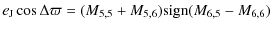
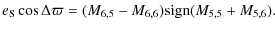
When
![]() one has
one has

where sign() is equal to -1 if the argument of the function is negative, +1 if it is positive and 0 if it is zero. Instead, when
Now, suppose that the amplitude corresponding to the g5 frequency is zero, i.e. M5,5=M6,5=0. Then, the dependence of Eq. (3) on
Let us now gradually increase the
amplitudes of the g5 mode, relative to that of the g6 one. This implies increasing M5,5 and M6,5 at the same rate, while keeping M5,6 and M6,6 fixed.
Initially, when M5,5 and M6,5 are small compared to M5,6 and
M6,6, all quantities
in Eqs. (6) and (7) are negative, and therefore the
evolution of the system follows an energy level curve of type I, along
which
![]() librates around
librates around ![]() .
The distance of this curve
from the equilibrium point, which we call amplitude of oscillation hereafter,
is directly proportional to M5,5 or M6,5.
.
The distance of this curve
from the equilibrium point, which we call amplitude of oscillation hereafter,
is directly proportional to M5,5 or M6,5.
Since
M5,6 < M6,6 and
M6,5 < M5,5, then when
M5,5 = M5,6 one has
M6,5 < M6,6. This implies that increasing the amplitude of the g5 mode eventually brings us to the situation where M5,5 becomes larger than M5,6, but M6,5 is still less than M6,6. Now the value of
![]() at
at
![]() i.e.
M5,5-M5,6 becomes positive. When additionally
i.e.
M5,5-M5,6 becomes positive. When additionally
![]() its value remains negative, i.e.
-(M5,5+M5,6). Thus, the system now evolves on
an energy curve of type II,
along which
its value remains negative, i.e.
-(M5,5+M5,6). Thus, the system now evolves on
an energy curve of type II,
along which
![]() circulates. Notice that the value of
circulates. Notice that the value of
![]() at
at
![]() remains negative,
while the value at
remains negative,
while the value at
![]() jumps from
-(M6,5+M6,6) to
(M6,5+M6,6). Thus, the level curve in
the right panel of Fig. 3 flips from one looping
around the equilibrium point at
jumps from
-(M6,5+M6,6) to
(M6,5+M6,6). Thus, the level curve in
the right panel of Fig. 3 flips from one looping
around the equilibrium point at
![]() to one looping around the
equilibrium at
to one looping around the
equilibrium at
![]() .
.
Further increasing the amplitude of the g5 mode
relative to that of the g6 mode eventually results in M6,5 also becoming
larger than M6,6. Now, all quantities in Eqs. (6) and (7) are positive, which means the system follows an
energy level curve of type III, along which
![]() librates
around 0. Notice that the value of
librates
around 0. Notice that the value of
![]() at
at
![]() jumps from
-(M5,5+M5,6) to
(M5,5+M5,6), which means that the level curve in the left
panel of Fig. 3 flips from one going around the
equilibrium point at
jumps from
-(M5,5+M5,6) to
(M5,5+M5,6), which means that the level curve in the left
panel of Fig. 3 flips from one going around the
equilibrium point at
![]() to one going around the equilibrium
at
to one going around the equilibrium
at
![]() .
.
Finally, when the amplitude of the g6 mode is zero, the
system is on the stable equilibrium at
![]() (the cross in
Fig. 3).
(the cross in
Fig. 3).
Below we discuss how the secular dynamics of the planets changes as they migrate away from each other and are also submitted to dynamical friction, exerted by the planetesimal population.
2.1 Migration and the evolution of the secular dynamics
Let's imagine two planets migrating, without
passing through any major mean motion resonance. A good example could
be Jupiter and Saturn migrating from a configuration with orbital
period ratio
![]() slightly higher than 2 to their current
configuration, with
slightly higher than 2 to their current
configuration, with
![]() slightly lower than 2.5.
slightly lower than 2.5.
The migration causes the semi-major axis ratio between the planets
to change. This affects the values of the coefficients Mj,k, since they depend explicitly on the above ratio; in turn,
this affects the global portrait of secular dynamics. However, if the migration
is slow enough, the amplitude of oscillation around the equilibrium
point is preserved as an adiabatic invariant (Neishtadt 1984;
Henrard 1993). More precisely, it can be demonstrated that the conserved quantity is
which is the action conjugate to
2.2 Dynamical friction and the evolution of the secular dynamics
Dynamical friction is the mechanism by which gravitating objects of different masses exchange energy so as to evolve towards an equipartition of energy of relative motion (Saslaw 1985). For a system of planets embedded in a massive population of small bodies, the eccentricities and inclinations of the former are damped, while those of the latter are excited (Stewart & Wetherill 1988).
In principle, each planet might suffer dynamical friction with different intensity, owing to a different location inside the planetesimal disk. However, the planets are connected to each other through their secular dynamics, so that dynamical friction, even if acting in an unbalanced way between the planets, turns out to have a systematic net effect.
![\begin{figure}
\par\resizebox{9cm}{!}{\includegraphics[angle=-90]{12876fg4.eps}}
\end{figure}](/articles/aa/full_html/2009/44/aa12876-09/img56.png)
|
Figure 4: Effect of eccentricity damping on the evolution of Jupiter and Saturn. In this experiment the damping force is applied to Saturn only. The top panel shows the coefficients M5,5 (filled circles), M5,6 (open circles), M6,5(filled triangles) and M6,6 (open triangles) as a function of time. The bottom panel shows the eccentricities of Saturn (open circles) and Jupiter (filled circles). |
| Open with DEXTER | |
To illustrate this point, consider again the Jupiter-Saturn system of
Fig. 3 and suppose that dynamical friction is applied
only to Saturn. The eccentricity of Saturn is damped, so the value of K is reduced. Consequently, the location of the two stable
equilibrium points has to move towards e=0. If the adiabatic
invariance of Eq. (8) held, the amplitude of oscillation
around the equilibrium point would be preserved, eventually turning a
libration of
![]() into a circulation. However, the adiabatic
invariance does not hold in this case. The reason is that dynamical
friction damps the eccentricity of Saturn, and therefore damps both
the M6,6 and the M6,5 coefficients. Since the M5,5 and
M6,5 coefficients are related, M5,5 is also damped. In other
words, the amplitude of oscillation around the equilibrium point is
damped, and so the value of J given in Eq. (8) decays with time.
into a circulation. However, the adiabatic
invariance does not hold in this case. The reason is that dynamical
friction damps the eccentricity of Saturn, and therefore damps both
the M6,6 and the M6,5 coefficients. Since the M5,5 and
M6,5 coefficients are related, M5,5 is also damped. In other
words, the amplitude of oscillation around the equilibrium point is
damped, and so the value of J given in Eq. (8) decays with time.
As a check, we have run a simple numerical experiment. We have
considered a Jupiter-Saturn system with semi-major axes 5.4 and 8.85,
with relatively eccentric orbits and large amplitude (
![]() )
of
apsidal libration around
)
of
apsidal libration around
![]() .
We have integrated
the orbits using the Wisdom-Holman (Wisdom & Holman 1991) method, with the code
Swift-WHM (Levison & Duncan 1994). We used a time-step of 0.1 y and
modified the equations of motion so that a damping term is included
for the eccentricity of Saturn only. Figure 4 shows the
result. The bottom panel shows the evolutions of the eccentricities
of the two planets, where
.
We have integrated
the orbits using the Wisdom-Holman (Wisdom & Holman 1991) method, with the code
Swift-WHM (Levison & Duncan 1994). We used a time-step of 0.1 y and
modified the equations of motion so that a damping term is included
for the eccentricity of Saturn only. Figure 4 shows the
result. The bottom panel shows the evolutions of the eccentricities
of the two planets, where ![]() is represented by open circles and
is represented by open circles and
![]() by filled circles: both are damped and decay with time at the
same rate. The top panel shows the amplitudes of the coefficients of
Eq. (2), i.e. M5,5 (filled circles), M5,6(open circles), M6,5 (filled triangles) and M6,6 (open
triangles), computed at six different points in time. The
computations were performed, by applying Fourier analysis to the time
series produced in six short-time integrations, where no
eccentricity damping was applied. As one can see, all coefficients
decrease with time at comparable rates.
by filled circles: both are damped and decay with time at the
same rate. The top panel shows the amplitudes of the coefficients of
Eq. (2), i.e. M5,5 (filled circles), M5,6(open circles), M6,5 (filled triangles) and M6,6 (open
triangles), computed at six different points in time. The
computations were performed, by applying Fourier analysis to the time
series produced in six short-time integrations, where no
eccentricity damping was applied. As one can see, all coefficients
decrease with time at comparable rates.
Thus, we conclude that, whatever the initial configuration of the
planets, smooth migration and dynamical friction cannot increase the
amplitude of the g5 term and cannot turn the libration of
![]() into a circulation. This result will be relevant in the
next section.
into a circulation. This result will be relevant in the
next section.
3 The effect of the passage through the 2:1 resonance
We now consider the migration of Jupiter and Saturn, initially on quasi-circular orbits, through their mutual 2:1 mean motion resonance. Tsiganis et al. (2005) argued that this passage through the resonance is responsible for the acquisition of the current eccentricities of the two planets.
Figure 5 shows the effect of the passage through this
resonance, starting from circular orbits. The simulation is again done
using the Swift-WHM integrator, but in this case
the equations of motion are modified so as to induce radial migration
to the planets, with a rate decaying as
![]() .
No
eccentricity damping is imposed. In practice, at every
timestep h the velocity of each planet is multiplied by a quantity
.
No
eccentricity damping is imposed. In practice, at every
timestep h the velocity of each planet is multiplied by a quantity
![]() ,
with
,
with ![]() being proportional to
being proportional to
![]() .
For
Jupiter
.
For
Jupiter ![]() is negative and for
Saturn it is positive, so that the two planets migrate inwards and outwards
respectively, as observed in realistic N-body simulations (Fernandez
& Ip 1984; Hahn & Malhotra 1999;
Gomes et al. 2004). We chose
is negative and for
Saturn it is positive, so that the two planets migrate inwards and outwards
respectively, as observed in realistic N-body simulations (Fernandez
& Ip 1984; Hahn & Malhotra 1999;
Gomes et al. 2004). We chose ![]() Myr.
Myr.
![\begin{figure}
\par\resizebox{9cm}{!}{\includegraphics[angle=-90]{12876fg5.eps}}
\end{figure}](/articles/aa/full_html/2009/44/aa12876-09/img64.png)
|
Figure 5: The evolution of Jupiter and Saturn, as they pass across their mutual 2:1 resonance. In the bottom panel, Saturn's eccentricity is the upper curve and Jupiter's is the lower one. |
| Open with DEXTER | |
| Figure 6: Similar to Fig. 3 but after the 2:1 resonance crossing. |
|
| Open with DEXTER | |
The top panel of Fig. 5 shows the ratio of the orbital
periods of Saturn (![]() )
and Jupiter (
)
and Jupiter (![]() )
as a function of
time. We stop the simulation well before
)
as a function of
time. We stop the simulation well before
![]() achieves the
current value, to emphasise the effect of the 2:1 resonance
crossing. The middle panel shows
achieves the
current value, to emphasise the effect of the 2:1 resonance
crossing. The middle panel shows
![]() as a function of
time. The bottom panel shows the evolutions of the eccentricities of
Jupiter and Saturn, where the bottom trajectory corresponds to Jupiter
and the top curve corresponds to Saturn. We notice that the orbital
period ratio abruptly jumps across the value of 2. Correspondingly,
the eccentricities of Saturn and Jupiter jump to
as a function of
time. The bottom panel shows the evolutions of the eccentricities of
Jupiter and Saturn, where the bottom trajectory corresponds to Jupiter
and the top curve corresponds to Saturn. We notice that the orbital
period ratio abruptly jumps across the value of 2. Correspondingly,
the eccentricities of Saturn and Jupiter jump to ![]() 0.07 and
0.07 and ![]() 0.045, which, as noticed by Tsiganis et al. (2005), are
quite close to the current mean eccentricities of the two
planets. During the subsequent migration, the eccentricity of Saturn
increases somewhat and that of Jupiter decreases respectively. The
two planets enter into apsidal anti-alignment (i.e.
0.045, which, as noticed by Tsiganis et al. (2005), are
quite close to the current mean eccentricities of the two
planets. During the subsequent migration, the eccentricity of Saturn
increases somewhat and that of Jupiter decreases respectively. The
two planets enter into apsidal anti-alignment (i.e.
![]() librates around 180 degrees) shortly before the resonance passage and
the libration amplitude shrinks down to
librates around 180 degrees) shortly before the resonance passage and
the libration amplitude shrinks down to ![]()
![]() as the
eccentricities of the two planets grow. The crossing of the 2:1 does
not seem to significantly affect the libration amplitude, which
remains of the order of
as the
eccentricities of the two planets grow. The crossing of the 2:1 does
not seem to significantly affect the libration amplitude, which
remains of the order of ![]()
![]() during the
post-resonance-crossing migration (see also Cuk 2007). As a result of this narrow
libration amplitude, the eccentricities of Jupiter and Saturn do not
show any sign of secular oscillation. In practice, Jupiter and Saturn
are located at the stable equilibrium point of their secular dynamics,
as shown in Fig. 6. This is very different from the
current situation (compare with
Fig. 3). Table 3 reports the values of
the Mi,k coefficients of Eq. (2) at the end of
the simulation. The M5,5 and M6,5 coefficients, related to
the amplitude of oscillation around the equilibrium point as explained
in Sect. 2, are very small; they are more than an order
of magnitude smaller than their current values. As discussed in
Sect. 2.1, they would not increase during the
subsequent migration of the planets because they behave as adiabatic
invariants. Even worse, they would decrease if dynamical friction
were applied.
during the
post-resonance-crossing migration (see also Cuk 2007). As a result of this narrow
libration amplitude, the eccentricities of Jupiter and Saturn do not
show any sign of secular oscillation. In practice, Jupiter and Saturn
are located at the stable equilibrium point of their secular dynamics,
as shown in Fig. 6. This is very different from the
current situation (compare with
Fig. 3). Table 3 reports the values of
the Mi,k coefficients of Eq. (2) at the end of
the simulation. The M5,5 and M6,5 coefficients, related to
the amplitude of oscillation around the equilibrium point as explained
in Sect. 2, are very small; they are more than an order
of magnitude smaller than their current values. As discussed in
Sect. 2.1, they would not increase during the
subsequent migration of the planets because they behave as adiabatic
invariants. Even worse, they would decrease if dynamical friction
were applied.
Table 3: Coefficients Mj,k of the Jupiter-Saturn secular system at the end of the simulation illustrated in Fig. 5.
Table 4:
Values of M5,5 in Jupiter after the 2:1 resonance crossing with Saturn as a function of the migration e-folding time, ![]() .
.
Simulations that we performed assuming longer values of ![]() (i.e. slower migration rates) lead to the same result. The
eccentricities of Jupiter and Saturn after the 2:1 resonance crossing
are approximately the same as in Fig. 5. The amplitude of libration of
(i.e. slower migration rates) lead to the same result. The
eccentricities of Jupiter and Saturn after the 2:1 resonance crossing
are approximately the same as in Fig. 5. The amplitude of libration of
![]() is always between 6 and 15 degrees, with no apparent
correlation on
is always between 6 and 15 degrees, with no apparent
correlation on ![]() .
Table 4 recapitulates the results, for
what concerns the values of the M5,5 coefficient, which are
always comparably small. Thus, we conclude that the 2:1 resonance
crossing, although it explains the current mean values of the
eccentricities of Jupiter and Saturn, cannot by itself explain the
current secular dynamical structure of the system.
.
Table 4 recapitulates the results, for
what concerns the values of the M5,5 coefficient, which are
always comparably small. Thus, we conclude that the 2:1 resonance
crossing, although it explains the current mean values of the
eccentricities of Jupiter and Saturn, cannot by itself explain the
current secular dynamical structure of the system.
Let us now provide an interpretation of the behaviour observed in the simulation. The dynamics of two planets in the vicinity of a mean motion resonance can be studied following Michtchenko et al. (2008). For the 2:1 resonance, the fundamental angles of the problem are
The motion of the first angle is conjugated with the motion of the
angular momentum deficit K of the planets, defined in Eq. (1). The motion of the second angle is conjugated with the
motion of the quantity
![]() .
If the system is far from the
resonance, the motion of
.
If the system is far from the
resonance, the motion of
![]() can be averaged out. Then Kbecomes a constant of motion and the secular dynamics described in
the previous section is recovered. In particular, if the planets migrate slowly enough so that the
adiabatic invariance of J - see Eq. (8)
- holds, the amplitude of oscillation around the stable
equilibrium point of the secular dynamics has to remain constant.
However, as migration continues,
the approach to the mean motion resonance forces the location of the
equilibrium point to shift to higher eccentricity. Thus, by virtue of a
geometric effect, the apparent amplitude of libration of
can be averaged out. Then Kbecomes a constant of motion and the secular dynamics described in
the previous section is recovered. In particular, if the planets migrate slowly enough so that the
adiabatic invariance of J - see Eq. (8)
- holds, the amplitude of oscillation around the stable
equilibrium point of the secular dynamics has to remain constant.
However, as migration continues,
the approach to the mean motion resonance forces the location of the
equilibrium point to shift to higher eccentricity. Thus, by virtue of a
geometric effect, the apparent amplitude of libration of
![]() has to shrink as the eccentricities
increase. This is visible in Fig. 5 in the phase before the resonance crossing.
has to shrink as the eccentricities
increase. This is visible in Fig. 5 in the phase before the resonance crossing.
As the planets are approaching the resonance, the angle
![]() can
no longer be averaged out in a trivial way. However, an adiabatic
invariant can still be introduced, as long as the timescale
for the motion of
can
no longer be averaged out in a trivial way. However, an adiabatic
invariant can still be introduced, as long as the timescale
for the motion of
![]() is significantly shorter than that of
is significantly shorter than that of
![]() and that migration changes the system on even longer
time scales. This invariant is
and that migration changes the system on even longer
time scales. This invariant is

|
(10) |
where the integral is taken over a path describing the coupled evolution of K and
As shown in Michtchenko et al. (2008), for a pair of planets with
the Jupiter-Saturn mass ratio and
![]() ,
the dynamics of the 2:1 resonance presents one critical curve, or separatrix, for the
,
the dynamics of the 2:1 resonance presents one critical curve, or separatrix, for the
![]() degree of freedom and no critical curve for the
degree of freedom and no critical curve for the
![]() degree of freedom. Thus, when the resonance is reached
during the migration, the invariance of
degree of freedom. Thus, when the resonance is reached
during the migration, the invariance of ![]() is broken
(Neishtadt 1984), since the two time-scales of the motion are no more
well separated. As the planets are migrating in divergent
directions, they cannot be trapped in the resonance (Henrard &
Lemaître 1983). The resonant angle
is broken
(Neishtadt 1984), since the two time-scales of the motion are no more
well separated. As the planets are migrating in divergent
directions, they cannot be trapped in the resonance (Henrard &
Lemaître 1983). The resonant angle
![]() has to switch from
clockwise to anti-clockwise circulation. Correspondingly, the
quantity
has to switch from
clockwise to anti-clockwise circulation. Correspondingly, the
quantity ![]() has to jump to a higher value, that is the planets
acquire an angular momentum deficit. How this new angular
momentum deficit is partitioned between the two planets is difficult
to compute a priori, because the dynamics are fully four-dimensional
(i.e. two degrees of freedom) and, therefore, not integrable.
has to jump to a higher value, that is the planets
acquire an angular momentum deficit. How this new angular
momentum deficit is partitioned between the two planets is difficult
to compute a priori, because the dynamics are fully four-dimensional
(i.e. two degrees of freedom) and, therefore, not integrable.
| Figure 7:
Left: the evolution of
|
|
| Open with DEXTER | |
As shown in Fig. 7, there are clearly two regimes of
motion in the portraits
![]() and
and
![]() (remember that
(remember that
![]() and
and
![]() ). Before the resonance crossing (black dots),
the dynamics are confined in a narrow, off-centred region close to the
origin of the polar coordinates. After the resonance crossing (grey
dots), the dynamics fill a wide annulus, also asymmetric relative to
the axis
). Before the resonance crossing (black dots),
the dynamics are confined in a narrow, off-centred region close to the
origin of the polar coordinates. After the resonance crossing (grey
dots), the dynamics fill a wide annulus, also asymmetric relative to
the axis
![]() .
The curves in each panel are free hand
illustrations of the dynamics near and inside a first-order mean
motion resonance. The region filled by the black dots is
bound by the inner loop of the critical curve (labelled I in the
plot). The annulus filled by the grey dots is adhesive, at its inner
edge, to the outer loop of the critical curve. The jump in
eccentricity observed at the resonance crossing corresponds to
the passage from the region inside the inner loop to that outside the
outer loop.
.
The curves in each panel are free hand
illustrations of the dynamics near and inside a first-order mean
motion resonance. The region filled by the black dots is
bound by the inner loop of the critical curve (labelled I in the
plot). The annulus filled by the grey dots is adhesive, at its inner
edge, to the outer loop of the critical curve. The jump in
eccentricity observed at the resonance crossing corresponds to
the passage from the region inside the inner loop to that outside the
outer loop.
Thus, in practice, it is as if each planet saw its own resonance:
the one with critical angle
![]() for Jupiter and the one with
critical angle
for Jupiter and the one with
critical angle
![]() for Saturn. The two resonances are just two
slices of the same resonance, because only one critical curve exists
(Michtchenko et al. 2008). This is the reason why the
eccentricities of both planets jump simultaneously. The 2:1 resonance
is structured by the presence of a periodic orbit, along which
for Saturn. The two resonances are just two
slices of the same resonance, because only one critical curve exists
(Michtchenko et al. 2008). This is the reason why the
eccentricities of both planets jump simultaneously. The 2:1 resonance
is structured by the presence of a periodic orbit, along which
![]() and
and
![]() remain constant and are equal to 0 and
remain constant and are equal to 0 and ![]() respectively (Michtchenko et al. 2008). As
respectively (Michtchenko et al. 2008). As
![]() ,
the phase portrait of the
,
the phase portrait of the
![]() resonance and that of the
resonance and that of the
![]() resonance are rotated
by 180 degrees with respect to each other. Thus,
resonance are rotated
by 180 degrees with respect to each other. Thus, ![]() reaches a
maximum when
reaches a
maximum when
![]() and
and ![]() has a maximum when
has a maximum when
![]() .
Consequently,
when the planets reach their maximal eccentricities and the
.
Consequently,
when the planets reach their maximal eccentricities and the ![]() angles start to circulate anti-clockwise,
angles start to circulate anti-clockwise,
![]() has to be
has to be
![]()
![]() (see Fig. 7). It is evident that
the result of this transition through the resonance depends just on
the resonance topology and not on the migration rate, as long as the
latter is slow compared to the motion of the
(see Fig. 7). It is evident that
the result of this transition through the resonance depends just on
the resonance topology and not on the migration rate, as long as the
latter is slow compared to the motion of the ![]() angles (i.e. the adiabatic approximation holds, Neishtadt 1984).
angles (i.e. the adiabatic approximation holds, Neishtadt 1984).
After the resonance crossing, one can again average over
![]() and reduce the system to a one-degree of freedom
secular system. As
and reduce the system to a one-degree of freedom
secular system. As
![]() ,
Jupiter has to be on the
negative x-axis of a diagram like that of the left panel of
Fig. 6. Thus, the secular evolution of Jupiter will be
an oscillation around the stable equilibrium at
,
Jupiter has to be on the
negative x-axis of a diagram like that of the left panel of
Fig. 6. Thus, the secular evolution of Jupiter will be
an oscillation around the stable equilibrium at
![]() .
The amplitude of this oscillation depends on the value of the
eccentricity of Jupiter acquired at resonance crossing, relative
to the value of the stable equilibrium of the secular problem.
It turns out that, for the masses of Jupiter
and Saturn, these two values are almost the same. Thus, the amplitude
of oscillation is very small. We think that this is a coincidence and
that, in principle, the situation does not have to be
this way. In fact, we have verified numerically that the result depends
on the individual masses of both planets, even for the
same mass ratio. For instance, if the masses of Jupiter and Saturn are
both reduced by a factor of 100, the eccentricities of both planets jump to
.
The amplitude of this oscillation depends on the value of the
eccentricity of Jupiter acquired at resonance crossing, relative
to the value of the stable equilibrium of the secular problem.
It turns out that, for the masses of Jupiter
and Saturn, these two values are almost the same. Thus, the amplitude
of oscillation is very small. We think that this is a coincidence and
that, in principle, the situation does not have to be
this way. In fact, we have verified numerically that the result depends
on the individual masses of both planets, even for the
same mass ratio. For instance, if the masses of Jupiter and Saturn are
both reduced by a factor of 100, the eccentricities of both planets jump to
![]() 0.01 at resonance crossing, and this puts Jupiter
on a secular trajectory that brings
0.01 at resonance crossing, and this puts Jupiter
on a secular trajectory that brings ![]() down to 0; that is, the secular
motion is now at the boundary between type-I and type-II, as defined in
Sect. 2. This is caused by a different scaling of the jumps in
down to 0; that is, the secular
motion is now at the boundary between type-I and type-II, as defined in
Sect. 2. This is caused by a different scaling of the jumps in
![]() and
and ![]() with respect to the planetary masses and to a
different global secular dynamics in the vicinity of the resonance, which in turn is
caused by a different relative importance of the quadratic terms in the
masses.
with respect to the planetary masses and to a
different global secular dynamics in the vicinity of the resonance, which in turn is
caused by a different relative importance of the quadratic terms in the
masses.
Once the planets are placed relative to the portrait of their secular
dynamics, their destiny is fixed. As they move away from the mean
motion resonance, the secular portrait can change, in particular
because the near-resonant perturbation terms that are quadratic
in the masses rapidly decrease in amplitude. Hence the location of the
equilibrium points can change, but the planets have to follow them
adiabatically. This explains the slow monotonic growth of the eccentricity
of Saturn and the decay of that of Jupiter, observed in the top panel
of Fig. 5, while the amplitude of libration of
![]() does
not change (middle panel).
does
not change (middle panel).
4 Passage through multiple resonances
Since the passage of Jupiter and Saturn through the 2:1 resonance, starting from initially circular orbits, produces a secular system that is incompatible with the current one, we now explore the effects of the passage of these planets through a series of resonances. This is done to determine whether or not such evolution could increase the value of Mj,5 in both planets.
We place Jupiter and Saturn initially on quasi-circular orbits just outside their mutual 3:2 resonance. The choice of these initial conditions is motivated by the result that during the gas-disk phase, Saturn should have been trapped in the 3:2 resonance with Jupiter (Morbidelli et al. 2007; Pierens & Nelson 2008). Once the gas disappeared from the system, the two planets should have been extracted from the resonance at low eccentricity, by the interaction with the planetesimals, and subsequently start to migrate.
In the above setting, our planets are forced to migrate through the
5:3, 7:4, 2:1, 9:4 and 7:3 resonances, ending up close to their
current location in semi-major axis (i.e. slightly interior to the
5:2 resonance). In the migration equations we have chosen ![]() such that
it takes about 40 Myr to reach
such that
it takes about 40 Myr to reach
![]() although, as we saw
before, the migration timescale has little influence on the resonant
effects. The result of this experiment is shown in
Fig. 8, which is similar in format to
Fig. 5. The horizontal lines in the top panel denote the
positions of the resonances mentioned above. Notice a distinct jump
in the eccentricities of both planets at each resonance crossing. In
order to prevent the system from becoming unstable we applied
eccentricity damping to Saturn, so as to mimic the effect of dynamical
friction and so that the planets reach final eccentricities that are similar to the
current mean values of the two planets. The parameters for the simulation
depicted in Fig. 8 are
although, as we saw
before, the migration timescale has little influence on the resonant
effects. The result of this experiment is shown in
Fig. 8, which is similar in format to
Fig. 5. The horizontal lines in the top panel denote the
positions of the resonances mentioned above. Notice a distinct jump
in the eccentricities of both planets at each resonance crossing. In
order to prevent the system from becoming unstable we applied
eccentricity damping to Saturn, so as to mimic the effect of dynamical
friction and so that the planets reach final eccentricities that are similar to the
current mean values of the two planets. The parameters for the simulation
depicted in Fig. 8 are ![]() Myr and
Myr and
![]() yr-1.
The effect of damping is visible in the eccentricity evolution, after the 2:1 resonance
crossing; we will discuss the effect on the motion of
yr-1.
The effect of damping is visible in the eccentricity evolution, after the 2:1 resonance
crossing; we will discuss the effect on the motion of
![]() below.
below.
![\begin{figure}
\par\resizebox{9cm}{!}{\includegraphics[angle=-90]{12876fg8.eps}}
\end{figure}](/articles/aa/full_html/2009/44/aa12876-09/img95.png)
|
Figure 8: Like Fig. 5, but for Jupiter and Saturn evolving through a sequence of mean motion resonances, from just outside their mutual 3:2 commensurability up to their current location. |
| Open with DEXTER | |
The middle panel of Fig. 8 shows that the passage through
the 7:4 resonance significantly increases the libration amplitude of
![]() .
In fact, the amplitude of the M5,5 term in (2), increases from
.
In fact, the amplitude of the M5,5 term in (2), increases from
![]() before the
resonance crossing, to 0.019 after the crossing. However, the
passage through the 2:1 resonance shrinks the amplitude of
libration of
before the
resonance crossing, to 0.019 after the crossing. However, the
passage through the 2:1 resonance shrinks the amplitude of
libration of
![]() .
This happens because the 2:1 resonance crossing, as
we have seen in the previous section, does not enhance M5,5 (it
remains equal to 0.019 in this simulation) but
does enhance the overall eccentricities of the planets. As explained earlier, this causes the amplitude
of libration of
.
This happens because the 2:1 resonance crossing, as
we have seen in the previous section, does not enhance M5,5 (it
remains equal to 0.019 in this simulation) but
does enhance the overall eccentricities of the planets. As explained earlier, this causes the amplitude
of libration of
![]() to decrease.
to decrease.
Notice from Fig. 8 that, after the 2:1 resonance
crossing, the amplitude of libration of
![]() starts to
increase, slowly and monotonically. This is caused not by an enhancement
of the amplitude of oscillation around the equilibrium point of the
secular dynamics, but by the damping of the eccentricities of the
planets. It is the opposite of what was just described before: a
geometrical effect. In reality, the value of M5,5 is decreased to 0.015 (from 0.019) during this evolution. Hence, at
the end of the simulation, the amplitude of the g5 mode is
about a factor of 3 smaller than in the real secular dynamics of Jupiter
and Saturn. Without eccentricity damping, the amplitude of the g5mode would have remained equal to
starts to
increase, slowly and monotonically. This is caused not by an enhancement
of the amplitude of oscillation around the equilibrium point of the
secular dynamics, but by the damping of the eccentricities of the
planets. It is the opposite of what was just described before: a
geometrical effect. In reality, the value of M5,5 is decreased to 0.015 (from 0.019) during this evolution. Hence, at
the end of the simulation, the amplitude of the g5 mode is
about a factor of 3 smaller than in the real secular dynamics of Jupiter
and Saturn. Without eccentricity damping, the amplitude of the g5mode would have remained equal to ![]() 0.019, still much smaller
than in the current Jupiter-Saturn secular dynamics.
0.019, still much smaller
than in the current Jupiter-Saturn secular dynamics.
Several other experiments, where we slightly changed the initial conditions or
the migration speed ![]() ,
lead essentially to the same result. Thus,
we conclude that the migration of Jupiter and Saturn through a
sequence of mean motion resonances is not enough to achieve their
current secular configuration. A richer dynamics is required,
likely involving interactions with a third planet.
,
lead essentially to the same result. Thus,
we conclude that the migration of Jupiter and Saturn through a
sequence of mean motion resonances is not enough to achieve their
current secular configuration. A richer dynamics is required,
likely involving interactions with a third planet.
5 Three-planet dynamics
From the discussions and the examples reported above, it is quite clear that, to enhance the amplitudes of the g5 mode, it is necessary that the eccentricity of Saturn receives a kick that is not counterbalanced by a corresponding increase in the eccentricity of Jupiter (or vice versa). This would indeed move the planets away from the stable equilibrium point of their secular dynamics, thus enhancing the amplitude of oscillation around this point and, consequently, Mj,5. Given that Jupiter and Saturn are not alone in the outer solar system, in this section we investigate the effect that interactions with a third planet with a mass comparable to that of Uranus and Neptune, which we simply refer to as ``Uranus'', has on the Jupiter-Saturn pair. We first address the effects of the migration of Uranus on a quasi-circular orbit. Then we study the effects of its migration on an initially eccentric orbit and, finally, we address the problem of encounters among the planets.
5.1 Migration of Uranus on a quasi-circular orbit
The main mean motion resonance with Saturn that Uranus can go through is the 2:1. Thus, this is the resonance crossing that we focus on here. Given that, as we have seen in the previous sections, the effect of a passage through a mean motion resonance is quite insensitive to the migration rate, the initial location of the planets etc., the main issue that may potentially lead to different results is whether the crossing of the 2:1 Saturn-Uranus resonance happened before or after the putative crossing of the 2:1 Jupiter-Saturn resonance. Below we investigate each of these two cases.
We have performed a numerical experiment where we have the
crossing of the Saturn-Uranus resonance happen first, with Saturn and Jupiter having
initially a small orbital period ratio (
![]() ), and Uranus
and Saturn having an orbital period ratio
), and Uranus
and Saturn having an orbital period ratio
![]() .
The exact initial locations are not important, as long as they do not
change the order of the resonance crossings.
All planets initially have circular orbits. The three
planets are forced to migrate to their current positions with
.
The exact initial locations are not important, as long as they do not
change the order of the resonance crossings.
All planets initially have circular orbits. The three
planets are forced to migrate to their current positions with ![]() Myr. Eccentricity damping is imposed on Saturn and Uranus, to mimic
dynamical friction, with forces tuned such that, at the end of the
simulation, Uranus approximately reaches its current eccentricity.
Myr. Eccentricity damping is imposed on Saturn and Uranus, to mimic
dynamical friction, with forces tuned such that, at the end of the
simulation, Uranus approximately reaches its current eccentricity.
Figure 9 shows the result. The top panel shows the
pericentre q and apocentre Q of the planets which, from top to
bottom, are Uranus, Saturn and Jupiter respectively. The separation
among these curves gives a visual measure of the eccentricity of the
orbit of the respective planet. The middle panel
shows
![]() for Jupiter and Saturn.
for Jupiter and Saturn.
![\begin{figure}
\par\resizebox{9cm}{!}{\includegraphics[angle=-90]{12876fg9.eps}}
\end{figure}](/articles/aa/full_html/2009/44/aa12876-09/img100.png)
|
Figure 9: A three-planet migration simulation, in which both the 2:1 resonance between Uranus and Saturn and the 2:1 resonance between Saturn and Jupiter are crossed. |
| Open with DEXTER | |
In this simulation, Uranus crosses the 2:1 resonance with Saturn at
![]() Myr. This gives a kick to the eccentricity of Uranus (its
q,Q-curves abruptly separate from each other) and, to a lesser
extent, to the eccentricity of Saturn. This sudden increase in the
eccentricity of Saturn moves the stable equilibrium point of the
Jupiter-Saturn secular dynamics away from
Myr. This gives a kick to the eccentricity of Uranus (its
q,Q-curves abruptly separate from each other) and, to a lesser
extent, to the eccentricity of Saturn. This sudden increase in the
eccentricity of Saturn moves the stable equilibrium point of the
Jupiter-Saturn secular dynamics away from
![]() .
However, the eccentricity of Jupiter does not receive an
equivalent kick by this resonance crossing, so it remains close to
zero. Consequently, Jupiter must start evolving secularly along a
trajectory close to the boundary between type-I and type-II curves
(see Sect. 2); in other words
.
However, the eccentricity of Jupiter does not receive an
equivalent kick by this resonance crossing, so it remains close to
zero. Consequently, Jupiter must start evolving secularly along a
trajectory close to the boundary between type-I and type-II curves
(see Sect. 2); in other words
![]() .
This
is the reason why the amplitude of libration of
.
This
is the reason why the amplitude of libration of
![]() changes abruptly at the Uranus-Saturn resonance crossing, and reaches
an amplitude of
changes abruptly at the Uranus-Saturn resonance crossing, and reaches
an amplitude of ![]()
![]() .
.
The interim between 0.9 and 3.3 Myr is characterised by large, long-periodic,
oscillations of the eccentricity of Uranus, which correlate with the
modulation of the amplitude of libration of
![]() .
These
oscillations have a frequency equal to g5-g7, where g7 is
the new fundamental frequency that characterises the extension of (2) to a three-planet system. Soon after the
Uranus-Saturn resonance crossing, g5-g7 is
slow compared to the frequencies themselves and therefore the oscillations have large amplitude. As Uranus
departs from the resonance with Saturn, g7 decreases; at the
same time, g5 increases, since Jupiter approaches the 2:1 resonance with Saturn. Hence, the oscillations with frequency g5-g7
becomes faster and its amplitude deceases. This sequence of increasingly
shorter oscillations reduces the overall amplitude of libration of
.
These
oscillations have a frequency equal to g5-g7, where g7 is
the new fundamental frequency that characterises the extension of (2) to a three-planet system. Soon after the
Uranus-Saturn resonance crossing, g5-g7 is
slow compared to the frequencies themselves and therefore the oscillations have large amplitude. As Uranus
departs from the resonance with Saturn, g7 decreases; at the
same time, g5 increases, since Jupiter approaches the 2:1 resonance with Saturn. Hence, the oscillations with frequency g5-g7
becomes faster and its amplitude deceases. This sequence of increasingly
shorter oscillations reduces the overall amplitude of libration of
![]() to approximately 40 degrees.
to approximately 40 degrees.
At ![]() Myr, Jupiter and Saturn cross their mutual 2:1 mean
motion resonance, which has the effects that we discussed before. The
amplitude of M5,5 is roughly preserved in this resonance
crossing, as already illustrated in Sect. 4. Its value at
t=4 Myr is 0.010, much larger than in Sect. 3 but still about
a factor of four smaller than the current value. The M5,5
coefficient receives an additional small enhancement at
Myr, Jupiter and Saturn cross their mutual 2:1 mean
motion resonance, which has the effects that we discussed before. The
amplitude of M5,5 is roughly preserved in this resonance
crossing, as already illustrated in Sect. 4. Its value at
t=4 Myr is 0.010, much larger than in Sect. 3 but still about
a factor of four smaller than the current value. The M5,5
coefficient receives an additional small enhancement at ![]() Myr,
when Jupiter and Saturn cross their 7:3 resonance, but this does not change
the substance of the result.
Myr,
when Jupiter and Saturn cross their 7:3 resonance, but this does not change
the substance of the result.
To reverse the order of the resonance crossings, we have run a second
experiment, in which we placed Jupiter and Saturn just beyond their
2:1 resonance (
![]() ), on orbits typical of those achieved
by the 2:1 resonance crossing (see Sect. 3). This means
that Jupiter and Saturn are in apsidal libration around 180
), on orbits typical of those achieved
by the 2:1 resonance crossing (see Sect. 3). This means
that Jupiter and Saturn are in apsidal libration around 180
![]() ,
with an amplitude of the g5 mode that is small in both planets
compared to the current value (see Table 3). Uranus was
placed on a circular orbit at
,
with an amplitude of the g5 mode that is small in both planets
compared to the current value (see Table 3). Uranus was
placed on a circular orbit at
![]() .
Again the planets were
forced to migrate to their current locations, with
.
Again the planets were
forced to migrate to their current locations, with ![]() Myr. The
2:1 resonance crossing between Uranus and Saturn again kicked the
eccentricity of Saturn, which in turn enhanced the amplitude of the
g5 term. In this case, the final value of the M5,5 coefficient
was 0.014, i.e. similar to the previous
experiment.
Myr. The
2:1 resonance crossing between Uranus and Saturn again kicked the
eccentricity of Saturn, which in turn enhanced the amplitude of the
g5 term. In this case, the final value of the M5,5 coefficient
was 0.014, i.e. similar to the previous
experiment.
Given the above results, we conclude that, no matter when the
Uranus-Saturn 2:1 resonance crossing occurs, there is an enhancement
of the amplitude of the g5 term, as expected, but it is too small (by a factor of
![]() 3) to explain the current Jupiter-Saturn secular system. It appears that the mass of Uranus is too small to provide enough
eccentricity excitation on Saturn, when passing through a mean
motion resonance with it.
3) to explain the current Jupiter-Saturn secular system. It appears that the mass of Uranus is too small to provide enough
eccentricity excitation on Saturn, when passing through a mean
motion resonance with it.
5.2 Migration of Uranus on an eccentric orbit
In the current solar system, the proper frequency of perihelion of
Uranus, g7, is lower than g5 (3.1 and 4.3
![]() /yr,
respectively). If Uranus was much closer to Saturn, however, g7 had to be
much higher too. For instance, if Uranus were just outside the 2:1 resonance with Saturn (say
/yr,
respectively). If Uranus was much closer to Saturn, however, g7 had to be
much higher too. For instance, if Uranus were just outside the 2:1 resonance with Saturn (say
![]() AU and
AU and
![]() AU), g7 was
AU), g7 was ![]()
![]() /yr.
One might then wonder if, during the migration of Uranus, the g7=g5 secular resonance
could have occurred. On the other hand, if Jupiter was closer to Saturn, g5 would
have been higher as well;
/yr.
One might then wonder if, during the migration of Uranus, the g7=g5 secular resonance
could have occurred. On the other hand, if Jupiter was closer to Saturn, g5 would
have been higher as well;
![]() /yr if
/yr if
![]() .
Thus, the occurrence of the g5=g7 resonance depends on
the locations of both Jupiter and Uranus, relative to Saturn.
.
Thus, the occurrence of the g5=g7 resonance depends on
the locations of both Jupiter and Uranus, relative to Saturn.
![\begin{figure}
\par\resizebox{9cm}{!}{\includegraphics[angle=-90]{12876fg10.eps}}
\end{figure}](/articles/aa/full_html/2009/44/aa12876-09/img113.png)
|
Figure 10: A three-planet simulation, with Uranus initially on an eccentric orbit and migrating to its current location. No migration is imposed on Jupiter and Saturn. |
| Open with DEXTER | |
To see the effect of this secular resonance, we performed an idealised
experiment, in which we placed Jupiter at
![]() AU, Saturn at
AU, Saturn at
![]() AU and Uranus at
AU and Uranus at
![]() AU with an eccentricity of 0.25.
The initial eccentricities and
AU with an eccentricity of 0.25.
The initial eccentricities and
![]() for Jupiter and Saturn
were taken from a run, in which these planets passed through their
mutual 2:1 resonance and migrated up to the locations reported above.
Hence
for Jupiter and Saturn
were taken from a run, in which these planets passed through their
mutual 2:1 resonance and migrated up to the locations reported above.
Hence
![]() would librate with very small amplitude,
in the absence of Uranus. In this experiment the latter was forced to migrate
towards its current location, with
would librate with very small amplitude,
in the absence of Uranus. In this experiment the latter was forced to migrate
towards its current location, with ![]() Myr. No migration was
imposed on Jupiter and Saturn. Since initially
Myr. No migration was
imposed on Jupiter and Saturn. Since initially
![]() /yr
and g7>g5, the g5=g7 resonance crossing had to occur during
this simulation. No eccentricity damping was applied to any of the
planets in this run.
/yr
and g7>g5, the g5=g7 resonance crossing had to occur during
this simulation. No eccentricity damping was applied to any of the
planets in this run.
The result is shown in Fig. 10. In the first part of the
simulation (t<1.3 Myr) the amplitude of libration of
![]() ,
which is initially very small, suffers a large modulation,
correlated with the oscillations of the eccentricity of Uranus. The
dynamics here are analogous to what we described before, for the
interim between the two mean motion resonance crossings in
Fig. 9. At
,
which is initially very small, suffers a large modulation,
correlated with the oscillations of the eccentricity of Uranus. The
dynamics here are analogous to what we described before, for the
interim between the two mean motion resonance crossings in
Fig. 9. At ![]() Myr, the g5=g7 resonance is
crossed. This leads to an exchange of angular momentum between Uranus
and Jupiter. The eccentricity of Uranus decreases a bit, while the
value of the M5,5 coefficient is enhanced. As a response,
Myr, the g5=g7 resonance is
crossed. This leads to an exchange of angular momentum between Uranus
and Jupiter. The eccentricity of Uranus decreases a bit, while the
value of the M5,5 coefficient is enhanced. As a response,
![]() starts to circulate. The final value of M5,5 is 0.04, essentially matching the current value.
starts to circulate. The final value of M5,5 is 0.04, essentially matching the current value.
Although Jupiter has to be far from Saturn to have a genuine secular resonance crossing, we have found that more realistic simulations, in which Jupiter and Saturn are initially much closer to each other - so to be able to migrate in the correct proportion with respect to Uranus - can lead to interesting results as well. The reason is that, although from the beginning g7<g5, the two frequencies can become quasi-resonant; such interactions also allow for a significant transfer of eccentricity from Uranus to Jupiter and can excite the value of M5,5 up to the current figure.
However, the reader should be aware that, while the effect of mean
motion resonances is quite insensitive to parameters and initial
conditions, in the case of a secular resonance, the outcome depends
critically on a variety of issues. More precisely, the effects of the
g7=g5 resonance, or quasi-resonance, must depend on the
eccentricity of Uranus, the migration timescale ![]() and the
position of
and the
position of
![]() relative to
relative to
![]() ,
immediately before
this resonant interaction. The reason for the first dependence is
that
,
immediately before
this resonant interaction. The reason for the first dependence is
that ![]() sets the strength of the secular resonance. The
dependence on
sets the strength of the secular resonance. The
dependence on ![]() and
and
![]() has to do with the fact that the
timescale associated with a secular resonance is very long, of the
order of 1 Myr. Thus, migration through a secular resonance, unlike
migration through a mean motion resonance, is not an adiabatic
process, at least for values of
has to do with the fact that the
timescale associated with a secular resonance is very long, of the
order of 1 Myr. Thus, migration through a secular resonance, unlike
migration through a mean motion resonance, is not an adiabatic
process, at least for values of ![]() up to 10 Myr that we are
focusing on here. Thus, the time spent in the vicinity of the
resonance and the values of the phases at which the planets enter
the resonance have important impact on the resulting dynamics.
up to 10 Myr that we are
focusing on here. Thus, the time spent in the vicinity of the
resonance and the values of the phases at which the planets enter
the resonance have important impact on the resulting dynamics.
Given the above, we conclude that the secular interaction with an eccentric Uranus is a mechanism that is potentially capable of exciting the g5 mode in the Jupiter-Saturn system to the observed level, but this mechanism is quite un-generic. Moreover, if we invoked an eccentric Uranus to explain the origin of the Jupiter-Saturn dynamical architecture, we would still need to explain how Uranus got so eccentric in first place. Finally, the g7=g5 secular resonance cannot alone explain the excitation of the planetary inclinations, which will be discussed in Sect. 7. For all these reasons, we continue our search for a better mechanism and consider below the effect of planetary encounters.
5.3 Planetary encounters with Uranus
Close encounters between Uranus and Saturn could potentially be a very effective mechanism for kicking the eccentricity of Saturn and enhancing the amplitude of the g5 mode.
To investigate this, we have run a series of twenty simulations, where the
initial semi-major axes of Jupiter and Saturn were chosen such that
these two planets are just outside their 2:1 mean motion resonance
(
![]() ), on orbits typical of those achieved during the 2:1 resonance crossing (in apsidal anti-alignment with negligible
oscillation amplitude). Uranus was placed on an orbit with semi-major axis ranging
from 11.8 AU to 13.4 AU at 0.2 AU intervals, with an initial
eccentricity of 0.1. This value of the eccentricity is similar to
that achieved by Uranus under the secular forcing induced by
Jupiter and Saturn. The system was then allowed to evolve under the
mutual gravitational forces and external migration forces. For all simulations,
the e-folding time for the migration forces was set at 5 Myr. Eccentricity
damping was applied to Uranus and Saturn, the values being
), on orbits typical of those achieved during the 2:1 resonance crossing (in apsidal anti-alignment with negligible
oscillation amplitude). Uranus was placed on an orbit with semi-major axis ranging
from 11.8 AU to 13.4 AU at 0.2 AU intervals, with an initial
eccentricity of 0.1. This value of the eccentricity is similar to
that achieved by Uranus under the secular forcing induced by
Jupiter and Saturn. The system was then allowed to evolve under the
mutual gravitational forces and external migration forces. For all simulations,
the e-folding time for the migration forces was set at 5 Myr. Eccentricity
damping was applied to Uranus and Saturn, the values being
![]() /yr and
/yr and
![]() /yr.
The damping coefficient for Uranus was
assumed to be six times larger than that of Saturn because, in principle,
Uranus is more affected by the planetesimal disk than the gas-giants.
The strength of the damping term was calibrated so that the post-encounter
evolution of the eccentricity of Uranus follows the one seen in the full
N-body simulations of Tsiganis et al. (2005). These details are
not very important because we focus here on the final secular dynamics of
Jupiter and not on the final orbit of Uranus. The latter is very
sensitive to the prescription of damping, but not the former, as we
have seen in Sect. 2.2. Uranus was typically found to be scattered by Saturn (and sometimes by Jupiter).
The simulations were stopped once the phase of encounters among
the planets ended, either because Uranus was decoupled from the giant
planets, due to eccentricity damping, or because it was ejected
from the system.
/yr.
The damping coefficient for Uranus was
assumed to be six times larger than that of Saturn because, in principle,
Uranus is more affected by the planetesimal disk than the gas-giants.
The strength of the damping term was calibrated so that the post-encounter
evolution of the eccentricity of Uranus follows the one seen in the full
N-body simulations of Tsiganis et al. (2005). These details are
not very important because we focus here on the final secular dynamics of
Jupiter and not on the final orbit of Uranus. The latter is very
sensitive to the prescription of damping, but not the former, as we
have seen in Sect. 2.2. Uranus was typically found to be scattered by Saturn (and sometimes by Jupiter).
The simulations were stopped once the phase of encounters among
the planets ended, either because Uranus was decoupled from the giant
planets, due to eccentricity damping, or because it was ejected
from the system.
The simulations that yielded the best results in terms of
final M5,5 value are those with initial semi-major
axes of Uranus
![]() AU. In these successful simulations, a total of four or 20%,
the average final value of M5,5 was approximately 0.04, in very good agreement with the current configuration.
Figure 11 gives an example of evolution from one of
these successful runs, and is similar to Figs. 9 and 10. As seen in our results, initially placing Uranus
further away from Saturn results in encounters that are too weak to pump
up the g5 mode in Jupiter.
AU. In these successful simulations, a total of four or 20%,
the average final value of M5,5 was approximately 0.04, in very good agreement with the current configuration.
Figure 11 gives an example of evolution from one of
these successful runs, and is similar to Figs. 9 and 10. As seen in our results, initially placing Uranus
further away from Saturn results in encounters that are too weak to pump
up the g5 mode in Jupiter.
![\begin{figure}
\par\resizebox{8.8cm}{!}{\includegraphics[angle=-90]{12876fg11.eps}}
\end{figure}](/articles/aa/full_html/2009/44/aa12876-09/img126.png)
|
Figure 11: Example of an encounter between Uranus and Saturn. The plot is similar to Fig. 9. |
| Open with DEXTER | |
In summary, we conclude that encounters between Saturn and Uranus constitute an effective and quite generic mechanism for achieving a final secular evolution of the Jupiter-Saturn system that is consistent with their current state. Compared to all other mechanisms investigated in this paper, which either do not work or work only for an ad-hoc set of conditions, planet-planet scattering is our favoured solution to the problem of the origin of the secular architecture of the giant planet system. In Sect. 7 we provide further arguments in favour of this conclusion.
6 The Nice model and its alternatives
The work presented above shows that a combination of the effects provided by the 2:1 resonance crossing between Jupiter and Saturn and by encounters and/or secular interactions with an eccentric Uranus, can produce a Jupiter-Saturn system that behaves secularly like the real planets.
The 2:1 resonance crossing, the encounters among the planets and the high-eccentricity phases of Uranus and Neptune are essential ingredients of the Nice model (Tsiganis et al. 2005; Gomes et al. 2005; Morbidelli et al. 2007). Thus, we expect that this model not only reproduces the mean orbital eccentricities of the planets, as shown in Tsiganis et al. (2005), but also the correct architecture of secular modes. Curiously, this has never been properly checked before, and we do so in the following.
![\begin{figure}
\par\resizebox{8.8cm}{!}{\includegraphics[angle=-90]{12876fg12.eps}}
\end{figure}](/articles/aa/full_html/2009/44/aa12876-09/img127.png)
|
Figure 12: Sample evolution of the giant planets in the Nice model (from Gomes et al. 2005). Each planet is represented by a pair of curves, showing the time evolution of their perihelion and aphelion distance. |
| Open with DEXTER | |
In Fig. 12, the pericentre and apocentre distance of the
four giant planets are plotted as a function of time, in a
simulation taken from Gomes et al. (2005)
that
adequately reproduces the current positions of the giant planets. The
curve starting around 5 AU represents Jupiter, the one around
9 AU is
Saturn, the trajectory at 12 AU is Uranus (who ends up switching
positions with Neptune) and the uppermost curve at 16 AU is
Neptune
(who ends up closer to the Sun than Uranus). This plot is a
magnification around the time when Jupiter and Saturn cross their
2:1 resonance and the system becomes unstable. The plot shows the
phase
until all encounters had stopped, which in this case happened when the
period ratio between Jupiter and Saturn was
![]() .
The
final semi-major axes of the four planets are
.
The
final semi-major axes of the four planets are
![]() ,
so that the largest
``error'' is in Saturn's orbit. A Fourier spectrum of Jupiter's
eccentricity at the end of the simulation gives
M5,5=0.027, and
M5,6=0.036. The amplitude of the g5 term is a bit small, but
well within a factor of 2 from the real value. Another Nice-model run
from the same Gomes et al. (2005) study gave an
essentially identical result. However, a third simulation gave
M5,5=0.059, which is larger than the real value. In a fourth
simulation, in which not only Saturn but also Jupiter encountered an
ice giant, a value close to the current one was again recoverd, namely
M5,5=0.037. Given the chaotic nature of planetary encounters
and that the resulting M5,5 values are close to the current one (0.044) or even larger (e.g. 0.059), we conclude that the Nice model
is able to reproduce the secular architecture of the Jupiter-Saturn
system.
,
so that the largest
``error'' is in Saturn's orbit. A Fourier spectrum of Jupiter's
eccentricity at the end of the simulation gives
M5,5=0.027, and
M5,6=0.036. The amplitude of the g5 term is a bit small, but
well within a factor of 2 from the real value. Another Nice-model run
from the same Gomes et al. (2005) study gave an
essentially identical result. However, a third simulation gave
M5,5=0.059, which is larger than the real value. In a fourth
simulation, in which not only Saturn but also Jupiter encountered an
ice giant, a value close to the current one was again recoverd, namely
M5,5=0.037. Given the chaotic nature of planetary encounters
and that the resulting M5,5 values are close to the current one (0.044) or even larger (e.g. 0.059), we conclude that the Nice model
is able to reproduce the secular architecture of the Jupiter-Saturn
system.
In principle, depending on the initial separations between Saturn and the innermost ice giant, the Nice model can also give planetary evolutions in which encounters between Saturn and an ice giant do not occur (only the ice giants encountering each other; see Tsiganis et al. 2005). These evolutions have been rejected already in Tsiganis et al. (2005), because they lead to final mean eccentricities (and inclinations) that are too low and an orbital separation between Saturn and Uranus that is too narrow at the end. They also lead to a value of M5,5 that is much too small compared to the current value because the 2:1 resonance crossing alone is not capable of pumping the excitation of the g5 mode, as we have seen earlier.
At this point, one might wonder whether the Nice model, in the version
with Saturn-Uranus encounters, is the only
model capable of this result. From the study reported in this paper,
it seems likely that encounters among planets might be sufficient to
excite the modes of the final secular system, without any need for
Jupiter and Saturn crossing their mutual 2:1 resonance. In
other words, one might envision a model where Jupiter and Saturn
formed on circular orbits, well separated from each other in the beginning,
so that
![]() was always larger than 2. These planets then had close
encounters with other planetary embryos, which at the end left them on
eccentric orbits with both the g5 and g6 modes excited.
was always larger than 2. These planets then had close
encounters with other planetary embryos, which at the end left them on
eccentric orbits with both the g5 and g6 modes excited.
A single encounter of an embryo with one planet would not work
because, by kicking the eccentricity of one planet and not of the
other, it would produce a secular system with
![]() (if the embryo encountered Saturn) or with
(if the embryo encountered Saturn) or with
![]() (if
the embryo encountered Jupiter). The real system is different from
these two extremes. However, multiple encounters with one planet or
with both of them should do the job. To achieve an estimate of the
mass of the planetary embryo that could excite the secular modes of
Jupiter and Saturn up to the observed values, we have run four sets of
four simulations each. In each run we considered Jupiter, Saturn and
one embryo, initially on circular orbits. The mass of the embryo
was 1, 5, 10 and 15 Earth masses respectively, for the four
sets of
simulations. The initial location of the embryo was
(if
the embryo encountered Jupiter). The real system is different from
these two extremes. However, multiple encounters with one planet or
with both of them should do the job. To achieve an estimate of the
mass of the planetary embryo that could excite the secular modes of
Jupiter and Saturn up to the observed values, we have run four sets of
four simulations each. In each run we considered Jupiter, Saturn and
one embryo, initially on circular orbits. The mass of the embryo
was 1, 5, 10 and 15 Earth masses respectively, for the four
sets of
simulations. The initial location of the embryo was
![]() AU,
8.0 AU, 10.1 AU, 10.7 AU, for the four simulations in each set,
whereas Jupiter and Saturn were initially at
AU,
8.0 AU, 10.1 AU, 10.7 AU, for the four simulations in each set,
whereas Jupiter and Saturn were initially at
![]() AU and
AU and
![]() AU in all cases. In most simulations, the embryo was
eventually ejected from the Solar System: in two runs the embryo
collided with Jupiter. The values of the M5,5 and M6,6coefficients for each set of simulations are reported in
Table 5. It turns out that the putative embryo had to be
massive, of the order of >
AU in all cases. In most simulations, the embryo was
eventually ejected from the Solar System: in two runs the embryo
collided with Jupiter. The values of the M5,5 and M6,6coefficients for each set of simulations are reported in
Table 5. It turns out that the putative embryo had to be
massive, of the order of >
![]() .
We stress that multiple embryos with the same total mass would not do
an equal job because the geometries of the encounters would be
randomised leading to dynamical friction instead of excitation. In
fact, we did the same experiment with 100 Mars mass objects instead of
a unique 10 Earth-mass object; it resulted in M5,5 and M6,6
being smaller than 0.001, demonstrating that an ensemble of small
objects could not have excited the relevant modes to their current
states. In conclusion, for the excitation of the M5,5 mode
to reach its current value, Jupiter and Saturn
should have encountered Uranus or Neptune or a putative third ice giant
of comparable mass. Therefore, for what concerns the excitation of the
secular Fourier modes of the planetary orbits, a generic scenario of
global instability and mutual scattering of the four giant planets, as
originally proposed by Thommes et al. (1999) would work;
the passage of Jupiter and Saturn through their mutual 2:1 resonance,
which is specific to the Nice model relative to Thommes et al. (1999) (or Thommes et al. 2007, in which Jupiter
and Saturn are initially locked in the 2:1 resonance) is not
necessary.
.
We stress that multiple embryos with the same total mass would not do
an equal job because the geometries of the encounters would be
randomised leading to dynamical friction instead of excitation. In
fact, we did the same experiment with 100 Mars mass objects instead of
a unique 10 Earth-mass object; it resulted in M5,5 and M6,6
being smaller than 0.001, demonstrating that an ensemble of small
objects could not have excited the relevant modes to their current
states. In conclusion, for the excitation of the M5,5 mode
to reach its current value, Jupiter and Saturn
should have encountered Uranus or Neptune or a putative third ice giant
of comparable mass. Therefore, for what concerns the excitation of the
secular Fourier modes of the planetary orbits, a generic scenario of
global instability and mutual scattering of the four giant planets, as
originally proposed by Thommes et al. (1999) would work;
the passage of Jupiter and Saturn through their mutual 2:1 resonance,
which is specific to the Nice model relative to Thommes et al. (1999) (or Thommes et al. 2007, in which Jupiter
and Saturn are initially locked in the 2:1 resonance) is not
necessary.
However, Pierens & Nelson (2008) showed that the only possible
final configuration achieved by Jupiter and Saturn in the gas disk is
in their mutual 3:2 resonance. Unless alternative evolutions have been
missed in that work, this result invalidates the initial planetary
configurations considered in Thommes et al. (1999, 2007) and supports
the Nice model, in particular in its newest
version described in Morbidelli et al. (2007), where
the four giant planets start locked in a quadruple resonance with
![]() .
.
Table 5: Values of M5,5 in Jupiter and M6,6 in Saturn after ejecting planetary embryos of various masses from various original locations.
7 Ice giants and inclination constraints
Up to now we have focused our discussion on the secular evolution of the eccentricities of Jupiter and Saturn. However, the outer Solar System has two additional planets: Uranus and Neptune, which introduce the additional frequencies g7 and g8 in the secular evolution of the eccentricities. Thus, one should also be concerned about the correct excitation of the g7 and g8 modes in all planets. In addition, the planets have a rich secular dynamics in inclination, associated with the regression of their nodes. The excitation of the correct modes in the inclinations is a problem as crucial as that of the eccentricities.
The reason that we did not discuss these issues so far is because considerations based solely on the secular evolution of the eccentricities of Jupiter and Saturn have proved enough to guide us towards a solution, which is also valid in the more general problem. That is, these planetary encounters that are necessary to explain the Jupiter-Saturn secular architecture, can also explain the excitation of the g7 and g8 modes i.e. Mj,7 and Mj,8, and of the inclinations of the planets.
The excitation of the g7 and g8 modes does not appear to be very constraining. During the Saturn-Uranus and Uranus-Neptune encounters, the eccentricities of the ice giants become typically much larger than the current values. Thus, the combination of encounters and dynamical friction can produce a wide range of amplitudes of the g7 and g8 modes, including the current amplitudes. But we cannot exclude that other mechanisms, such as a sequence of mutual resonance crossing, could have led to the correct amplitudes as well.
Conversely, the inclination excitation is particularly interesting because it provides a strong, additional argument in favour of a violent evolution of the planets that involves mutual close encounters. In fact, the planets should form on essentially co-planar orbits, for the same reasons for which they should form on circular orbits: low relative velocities with respect to the planetesimals in the disk are necessary for the rapid formation of their cores. Once the planets are formed, tidal interactions with the gas disk damp the residual inclinations of the planets (Lubow & Ogilvie 2001). After the disappearance of the gas, dynamical friction exerted by the remnant planetesimal disk would also damp the planetary inclinations. Thus, similar to the eccentricities, a relatively-late excitation mechanism is required to explain the inclinations of the planets. However, unlike the eccentricities, the passage across mean motion resonances does not significantly excite the inclinations because the resonant terms depending on the longitude of the nodes are at least quadratic in the inclinations. Secular resonances are also ineffective, if all planetary inclinations are initially low. The only mechanism by which inclinations can be efficiently increased is by close encounters. In fact, in the Nice model, the inclinations of Saturn, Uranus and Neptune, relative to the orbit of Jupiter, are well reproduced. A similar result holds also for the Thommes et al. (1999) model.
It is interesting to note that the eccentricities of the giant
planets are about twice as large as the inclinations (respectively
![]() 0.05 and
0.05 and ![]() 0.025 radians or
0.025 radians or ![]()
![]() ). This is
what one would expect, if both the eccentricities and the inclinations
had been acquired by a combination of gravitational scattering and dynamical
friction. Conversely, if encounters among the planets had never happened
and the eccentricities had been acquired through specific resonance crossings,
we would expect the planetary eccentricities to be much higher than the inclinations.
). This is
what one would expect, if both the eccentricities and the inclinations
had been acquired by a combination of gravitational scattering and dynamical
friction. Conversely, if encounters among the planets had never happened
and the eccentricities had been acquired through specific resonance crossings,
we would expect the planetary eccentricities to be much higher than the inclinations.
8 Conclusion
In this work we have demonstrated that the secular architecture of the giant planets, which have non-negligible eccentricities and inclinations and specific amplitudes of the modes in the eccentricity evolution of Jupiter and Saturn, could not have been achieved if the planets migrated smoothly through a planetesimal disk, as originally envisioned in Malhotra (1993; see also Malhotra 1995; Hahn & Malhotra 1999; Gomes et al. 2004). Thus, we believe that the community should no longer consider the smooth migration model as a valid template for the evolution of the solar system. Even repeated passages through mutual resonances, that would have happened if the planetary system was originally more compact than envisioned in Malhotra's model, could not account for the orbital architecture of the giant planets, as we observe them today.
Instead, the outer planetary system had to evolve in a more violent way, in which the gas giants encountered the ice giants, or other rogue planets of equivalent mass. In this respect, the correct templates for the planetary evolution are the Nice model or the Thommes et al. model (or variants of these two). As we noted above, the Nice model seems to be, so far, more coherent and consistent in all its facets. We remark that encounters among the planets have been shown to also be an effective mechanism for the capture of the systems of irregular satellites (Nesvorny et al. 2007). These arguments, which are different and independent ofthose reported in this paper, also support a violent evolution scenario of the outer solar system.
In a forthcoming paper we will investigate the orbital dynamics of the terrestrial planets in the context of the evolution of the giant planets that we have outlined in this work.
AcknowledgementsThis work is part of the Helmholtz Alliance's ``Planetary evolution and life'', which RB and AM thank for financial support. Exchanges between Nice and Thessaloniki have been funded by a PICS programme of France's CNRS, and R.B. thanks the host K.T. for his hospitality during a recent visit. RG thanks Brazil's CNPq and FAPERJ for financial support. H.F.L. thanks NASA's OSS and OPR programmes for support. Most of the simulations for this work were performed on the CRIMSON Beowulf cluster at OCA.
References
- Cuk, M. 2007, DPS, 39, 60
- D'Angelo, G., Lubow, S., & Bate, M. 2006 ApJ 652, 1698
- Fernandez, J. A., & Ip, W.-H. 1984, Icarus, 58, 109 [CrossRef] [NASA ADS]
- Goldreich, P., & Sari, R. 2003, ApJ, 585, 1024 [CrossRef] [NASA ADS]
- Goldreich, P., Lithwick, Y., & Sari, R. 2004, ApJ, 614, 497 [CrossRef] [NASA ADS]
- Gomes, R., Morbidelli, A., & Levison, H. 2004, Icarus, 170, 492 [CrossRef] [NASA ADS]
- Gomes, R., Levison, H., Tsiganis, K., & Morbidelli, A. 2005, Nature, 435, 466 [CrossRef] [NASA ADS]
- Hahn, J., & Malhotra, R. 1999, AJ, 117, 3041 [CrossRef] [NASA ADS]
- Henrard, J., & Lemaître, A. 1983, Icarus, 55, 482 [CrossRef] [NASA ADS]
- Henrard, J. 1993, in Dynamics Reported New series, 2, 117
- Kley, W., & Dirksen, G. 2006, A&A, 447, 369 [EDP Sciences] [CrossRef] [NASA ADS]
- Kokubo, E., & Ida, S. 1996, Icarus, 123, 180 [CrossRef] [NASA ADS]
- Kokubo, E., & Ida, S. 1998, Icarus, 131, 171 [CrossRef] [NASA ADS]
- Levison, H., & Duncan, M. 1994, Icarus, 108, 18 [CrossRef] [NASA ADS]
- Lubow, S., & Ogilvie, G. 2001, ApJ, 560, 997 [CrossRef] [NASA ADS]
- Malhotra, R. 1993, Nature, 365, 819 [CrossRef] [NASA ADS]
- Malhotra, R. 1995, AJ, 110, 420 [CrossRef] [NASA ADS]
- Masset, F., & Snellgrove, M. 2001, MNRAS, 320, 55 [CrossRef] [NASA ADS]
- Michtchenko, T., & Malhotra, R. 2004, Icarus, 168, 237 [CrossRef] [NASA ADS]
- Michtchenko, T., Beaugé, C., & Ferraz-Mello, S. 2008, MNRAS, 391, 215 [CrossRef] [NASA ADS]
- Morbidelli, A. 2002, Modern Celestial Mechanics - Aspects of Solar System Dynamics (Taylor & Francis, UK).
- Morbidelli, A., & Crida, A. 2007, Icarus, 191, 158 [CrossRef] [NASA ADS]
- Morbidelli, A., Tsiganis, K., Crida, A., Levison, H., & Gomes, R. 2007, AJ, 134, 1790 [CrossRef] [NASA ADS]
- Murray, C., & Dermott, S. 1999, Solar System Dynamics (Cambridge, UK: Cambridge University Press)
- Neishtadt, A. 1984, J. App. Math. Mech., 48, 133 [CrossRef]
- Nelson, R. 2005, A&A, 443 1067
- Nesvorný, D., Vokrouhlický, D., & Morbidelli, A. 2007, AJ, 133, 1962 [CrossRef] [NASA ADS]
- Nobili, A., Milani, A., & Carpino, M. 1989, A&A, 210, 313 [NASA ADS]
- Pierens, A., & Nelson, R. 2008, A&A, 482, 333 [EDP Sciences] [CrossRef] [NASA ADS]
- Saslaw, W. 1985, ApJ, 297, 49 [CrossRef] [NASA ADS]
- Stewart, G., & Wetherill, G. 1988, Icarus, 74, 542 [CrossRef] [NASA ADS]
- Tsiganis, K., Gomes, R., Morbidelli, A., & Levison, H. 2005, Nature, 435, 459 [CrossRef] [NASA ADS]
- Thommes, E., Duncan, M., & Levison, H. 1999, Nature, 402, 635 [CrossRef] [NASA ADS]
- Thommes, E., Nilsson, L., & Murray, N. 2007, ApJ, 656, 25 [CrossRef] [NASA ADS]
- Wisdom, J., & Holman, M. 1991, AJ, 102, 1528 [CrossRef] [NASA ADS]
All Tables
Table 1: Frequencies and phases for the secular evolution of Jupiter and Saturn on their current orbits.
Table 2: Coefficients Mj,k of the Lagrange-Laplace solution for the Jupiter-Saturn system. The coefficients of the terms with frequencies other than g5 and g6 are omitted.
Table 3: Coefficients Mj,k of the Jupiter-Saturn secular system at the end of the simulation illustrated in Fig. 5.
Table 4:
Values of M5,5 in Jupiter after the 2:1 resonance crossing with Saturn as a function of the migration e-folding time, ![]() .
.
Table 5: Values of M5,5 in Jupiter and M6,6 in Saturn after ejecting planetary embryos of various masses from various original locations.
All Figures
|
|
Figure 1: The evolution of Jupiter (bullets) and Saturn (crosses) in the gas disk. Taken from Morbidelli & Crida (2007), but reproducing the evolution shown in Masset & Snellgrove (2001). |
| Open with DEXTER | |
| In the text | |
|
|
Figure 2: The evolution of the eccentricities of Jupiter (bullet) and Saturn (crosses) as they migrate through a 50 Earth masses planetesimal disk. From Gomes et al. (2004). |
| Open with DEXTER | |
| In the text | |
| |
Figure 3:
Global illustration of the secular dynamics of the
Jupiter-Saturn system. The bullets
represent the current values of |
| Open with DEXTER | |
| In the text | |
|
|
Figure 4: Effect of eccentricity damping on the evolution of Jupiter and Saturn. In this experiment the damping force is applied to Saturn only. The top panel shows the coefficients M5,5 (filled circles), M5,6 (open circles), M6,5(filled triangles) and M6,6 (open triangles) as a function of time. The bottom panel shows the eccentricities of Saturn (open circles) and Jupiter (filled circles). |
| Open with DEXTER | |
| In the text | |
|
|
Figure 5: The evolution of Jupiter and Saturn, as they pass across their mutual 2:1 resonance. In the bottom panel, Saturn's eccentricity is the upper curve and Jupiter's is the lower one. |
| Open with DEXTER | |
| In the text | |
| |
Figure 6: Similar to Fig. 3 but after the 2:1 resonance crossing. |
| Open with DEXTER | |
| In the text | |
| |
Figure 7:
Left: the evolution of
|
| Open with DEXTER | |
| In the text | |
|
|
Figure 8: Like Fig. 5, but for Jupiter and Saturn evolving through a sequence of mean motion resonances, from just outside their mutual 3:2 commensurability up to their current location. |
| Open with DEXTER | |
| In the text | |
|
|
Figure 9: A three-planet migration simulation, in which both the 2:1 resonance between Uranus and Saturn and the 2:1 resonance between Saturn and Jupiter are crossed. |
| Open with DEXTER | |
| In the text | |
|
|
Figure 10: A three-planet simulation, with Uranus initially on an eccentric orbit and migrating to its current location. No migration is imposed on Jupiter and Saturn. |
| Open with DEXTER | |
| In the text | |
|
|
Figure 11: Example of an encounter between Uranus and Saturn. The plot is similar to Fig. 9. |
| Open with DEXTER | |
| In the text | |
|
|
Figure 12: Sample evolution of the giant planets in the Nice model (from Gomes et al. 2005). Each planet is represented by a pair of curves, showing the time evolution of their perihelion and aphelion distance. |
| Open with DEXTER | |
| In the text | |
Copyright ESO 2009
Current usage metrics show cumulative count of Article Views (full-text article views including HTML views, PDF and ePub downloads, according to the available data) and Abstracts Views on Vision4Press platform.
Data correspond to usage on the plateform after 2015. The current usage metrics is available 48-96 hours after online publication and is updated daily on week days.
Initial download of the metrics may take a while.