| Issue |
A&A
Volume 507, Number 2, November IV 2009
|
|
|---|---|---|
| Page(s) | 861 - 879 | |
| Section | Interstellar and circumstellar matter | |
| DOI | https://doi.org/10.1051/0004-6361/200912325 | |
| Published online | 24 September 2009 | |
A&A 507, 861-879 (2009)
PROSAC: a submillimeter array survey of low-mass protostars
II. The mass evolution of envelopes, disks, and stars from the Class
0 through I stages![[*]](/icons/foot_motif.png)
J. K. Jørgensen1 - E. F. van Dishoeck2,3 - R. Visser2 - T. L. Bourke4 - D. J. Wilner4 - D. Lommen2 - M. R. Hogerheijde2 - P. C. Myers4
1 - Argelander-Institut für Astronomie, University of Bonn,
Auf dem Hügel 71, 53121 Bonn, Germany
2 - Leiden Observatory,
Leiden University, PO Box 9513, 2300 RA Leiden, The Netherlands
3 - Max-Planck Institut für Extraterrestrische Physik,
Giessenbachstrasse 1, 85748 Garching, Germany
4 -
Harvard-Smithsonian Center for Astrophysics, 60 Garden Street MS-42,
Cambridge, MA 02138, USA
Received 14 April 2009 / Accepted 8 September 2009
Abstract
Context. The key question about early protostellar evolution
is how matter is accreted from the large-scale molecular cloud, through
the circumstellar disk onto the central star.
Aims. We constrain the masses of the envelopes, disks, and
central stars of a sample of low-mass protostars and compare the
results to theoretical models for the evolution of young stellar
objects through the early protostellar stages.
Methods. A sample of 20 Class 0 and I protostars
has been observed in continuum at (sub)millimeter wavelengths at high
angular resolution (typically 2
![]() )
with the submillimeter array. Using detailed dust radiative transfer
models of the interferometric data, as well as single-dish continuum
observations, we have developed a framework for disentangling the
continuum emission from the envelopes and disks, and from that
estimated their masses. For the Class I sources in the sample HCO+ 3-2 line
emission was furthermore observed with the submillimeter array. Four of
these sources show signs of Keplerian rotation, making it possible to
determine the masses of the central stars. In the other sources the
disks are masked by optically thick envelope and outflow emission.
)
with the submillimeter array. Using detailed dust radiative transfer
models of the interferometric data, as well as single-dish continuum
observations, we have developed a framework for disentangling the
continuum emission from the envelopes and disks, and from that
estimated their masses. For the Class I sources in the sample HCO+ 3-2 line
emission was furthermore observed with the submillimeter array. Four of
these sources show signs of Keplerian rotation, making it possible to
determine the masses of the central stars. In the other sources the
disks are masked by optically thick envelope and outflow emission.
Results. Both Class 0 and I protostars are surrounded by disks with typical masses of about 0.05 ![]() ,
although significant scatter is seen in the derived disk masses for
objects within both evolutionary stages. No evidence is found for a
correlation between the disk mass and evolutionary stage of the young
stellar objects. This contrasts the envelope mass, which decreases
sharply from
,
although significant scatter is seen in the derived disk masses for
objects within both evolutionary stages. No evidence is found for a
correlation between the disk mass and evolutionary stage of the young
stellar objects. This contrasts the envelope mass, which decreases
sharply from ![]() 1
1 ![]() in the Class 0 stage to
in the Class 0 stage to ![]() 0.1
0.1 ![]() in the Class I stage. Typically, the disks have masses that are 1-10%
of the corresponding envelope masses in the Class 0 stage and
20-60% in the Class I stage. For the Class I sources for
which Keplerian rotation is seen, the central stars contain 70-98% of
the total mass in the star-disk-envelope system, confirming that these
objects are late in their evolution through the embedded protostellar
stages, with most of the material from the ambient envelope accreted
onto the central star. Theoretical models tend to overestimate the disk
masses relative to the stellar masses in the late Class I stage.
in the Class I stage. Typically, the disks have masses that are 1-10%
of the corresponding envelope masses in the Class 0 stage and
20-60% in the Class I stage. For the Class I sources for
which Keplerian rotation is seen, the central stars contain 70-98% of
the total mass in the star-disk-envelope system, confirming that these
objects are late in their evolution through the embedded protostellar
stages, with most of the material from the ambient envelope accreted
onto the central star. Theoretical models tend to overestimate the disk
masses relative to the stellar masses in the late Class I stage.
Conclusions. The results argue in favor of a picture in which
circumstellar disks are formed early during the protostellar evolution
(although these disks are not necessarily rotationally supported) and
rapidly process material accreted from the larger scale envelope onto
the central star.
Key words: stars: formation - stars: circumstellar matter - stars: planetary systems: protoplanetary disks - radiative transfer
1 Introduction
The fundamental problem in studies of the evolution of low-mass young
stellar objects is how material is accreted from the larger scale
envelope through the protoplanetary disk onto the central star - and,
in particular, what evolutionary time-scales determine the formation
and growth of the disk and star and the dissipation of envelopes. Our
theoretical understanding of the evolution of YSOs has typically
relied on the coupling between theoretical studies and empirical
schemes, based, for example, on the spectral energy distributions or
colors or on indirect measures, e.g., of the accretion rates. The most
commonly used distinction between the embedded Class 0 and I
protostars is that the former emit more than 0.5% of their luminosity
at wavelengths longer than 350 ![]() m. This in turn is thought to
reflect that they have accreted less than half of their final mass
(e.g., André et al. 2000,1993), but few hard constraints on the
actual evolution of the matter through the embedded protostellar
stages exist. Direct measurements of the stellar, disk, and envelope
masses during these pivotal stages can place individual protostars in
their proper evolutionary context by addressing questions such as what
fraction of the initial core mass has been accreted onto the central
star, what fraction is being carried away by the action of the
protostellar outflows and what fraction has (so-far) ended up in a
disk. In this paper, we analyze single-dish and interferometric
observations of emission from dust around a sample of 20 Class 0 and I
low-mass protostars, as well as observations of a dense gas tracer,
HCO+ 3-2, for the Class I sources. By interpreting continuum data
using dust radiative transfer models, we disentangle the contributions
from the envelopes and disks to the emission and estimate their
masses. Together with stellar masses inferred from Keplerian rotation
in resolved line maps (see also Lommen et al. 2008; Brinch et al. 2007), we
directly constrain the evolution of matter during the earliest
embedded stages of young stellar objects.
m. This in turn is thought to
reflect that they have accreted less than half of their final mass
(e.g., André et al. 2000,1993), but few hard constraints on the
actual evolution of the matter through the embedded protostellar
stages exist. Direct measurements of the stellar, disk, and envelope
masses during these pivotal stages can place individual protostars in
their proper evolutionary context by addressing questions such as what
fraction of the initial core mass has been accreted onto the central
star, what fraction is being carried away by the action of the
protostellar outflows and what fraction has (so-far) ended up in a
disk. In this paper, we analyze single-dish and interferometric
observations of emission from dust around a sample of 20 Class 0 and I
low-mass protostars, as well as observations of a dense gas tracer,
HCO+ 3-2, for the Class I sources. By interpreting continuum data
using dust radiative transfer models, we disentangle the contributions
from the envelopes and disks to the emission and estimate their
masses. Together with stellar masses inferred from Keplerian rotation
in resolved line maps (see also Lommen et al. 2008; Brinch et al. 2007), we
directly constrain the evolution of matter during the earliest
embedded stages of young stellar objects.
The formation of a circumstellar disk is clearly a key event in the evolution of young stellar objects, providing the route through which material is accreted from the large-scale envelope onto the central star. Theoretically a rotationally supported circumstellar disk is expected to form during the collapse of a dense core due to its initial angular momentum: material falling in from the outer regions of the core will be deflected away from the central star into a flat circumstellar disk structure at the ``centrifugal radius'' where gravity is balanced by rotation (e.g., Cassen & Moosman 1981; Terebey et al. 1984; Basu 1998; Ulrich 1976). The centrifugal radius will grow in time, with the exact pace depending on the distribution of angular momentum in the infalling core, e.g., whether it can be described as solid-body rotation (e.g., Terebey et al. 1984) or as differential rotation as expected in magnetized infalling cores (e.g., Basu 1998). Even earlier in the evolution of low-mass YSOs, an unstable pseudo-disk may develop as magnetic fields in the core deflect infalling material away from the radial direction toward the central disk plane (Galli & Shu 1993b,a).
The existence of circumstellar disks has been used to solve the so-called ``luminosity problem'' (e.g. Kenyon et al. 1990) in which embedded young stellar objects are observed to be under-luminous compared to the expected luminosity due to release of gravitational energy under constant mass accretion onto the central star. The solution proposed by Kenyon et al. (1990) is that material is accreted onto the circumstellar disk (and thus at larger radii with a smaller release of gravitational energy) and from there episodically onto the central star, e.g., related to the observed FU Orionis outbursts. The recent compilation of YSO luminosities from the Spitzer Space Telescope ``Cores to Disks (c2d)'' legacy program (Evans et al. 2009) shows that even the most deeply embedded YSOs are under-luminous compared to the predictions from models - perhaps suggesting that already in these early phases material is not accreted directly on to the central protostar, but rather accumulated either in a circumstellar disk or accreted in another episodic manner.
The main issue about inferring the properties of circumstellar disks
around embedded YSOs remains to disentangle the contribution from the
larger scale envelopes and circumstellar disks. The continuum emission
from dust on the other hand provides an optically thin tracer, whose
strength mainly depends on the column density and temperature of the
emitting material - and thus potentially provides a direct probe of
the dust mass of envelope and/or disks if these can be separated.
High angular resolution line observations provide a means to complete
the picture of the structure of young stellar objects and their
evolution by constraining the dynamical structure of the inner
envelope and disk and through that infer the central stellar masses
(e.g., Brown & Chandler 1999; Lommen et al. 2008; Brinch et al. 2007). In particular,
aperture synthesis observations at submillimeter wavelengths are
important for this goal: the higher excitation transitions of common
molecules such as HCO+, HCN and CS observed at 1 mm and shorter
wavelengths, probe densities ![]() 105 cm-3 and temperatures
105 cm-3 and temperatures
![]() 25 K (e.g., Evans 1999) and are thus much less sensitive
to the structure of the outer envelope/ambient cloud compared to
ground-state and low-excitation transitions observable at longer
wavelengths.
25 K (e.g., Evans 1999) and are thus much less sensitive
to the structure of the outer envelope/ambient cloud compared to
ground-state and low-excitation transitions observable at longer
wavelengths.
For more evolved YSOs in fairly isolated regions, single-dish
continuum observations have been used for comparative studies of
statistically significant samples of sources
(e.g., Andrews & Williams 2005; André & Montmerle 1994; Beckwith et al. 1990; Andrews & Williams 2007b). Subarcsecond
resolution imaging using (sub)millimeter wave interferometers has been
done for smaller samples of objects
(e.g., Looney et al. 2000; Mundy et al. 1996; Lay et al. 1994; Hogerheijde et al. 1997b). For
embedded protostars, the issue arises that both the disks and
envelopes may contribute significantly to the emission within the
typical single-dish beam and for such sources, interferometric imaging
is needed to address the dust distribution on the size scales where
disks may be forming. Keene & Masson (1990) demonstrated the potential of
such high angular resolution millimeter observations using data from
the OVRO millimeter array: by comparing the interferometric data to
models for the collapsing envelope around the L1551-IRS5 Class I
protostar, inferred from modeling its SED, Keene & Masson found
that a central unresolved component was required to explain the
observed brightness profiles in the interferometric data, such as
expected from a central circumstellar disk. In the case of L1551-IRS5,
this compact component accounts for about 50% of the total dust
continuum emission - or if interpreted in the context of a
circumstellar disk and envelope - a circumstellar disk containing
about 20-25% of the total mass in the
system. Hogerheijde et al. (1998,1997a) used the OVRO Millimeter
Array to survey the continuum and line emission at 3 mm from a sample
of 9 Class I protostellar sources. They showed that most of the
continuum emission was associated with a compact, unresolved
(<3
![]() )
component. More recently these kind of studies have seen
significant progress with the advent of new data and more detailed
dust radiative transfer models
(e.g., Eisner et al. 2005; Schöier et al. 2004; Jørgensen 2004; Brinch et al. 2007; Hogerheijde & Sandell 2000; Jørgensen et al. 2005a; Looney et al. 2003; Jørgensen et al. 2004a; Lommen et al. 2008). In
many cases, evidence is found for similarly compact components -
although the exact interpretation of their nature still depends on
assumptions about the properties of the larger scale envelopes. Still,
despite these efforts the studied samples have been limited to at most
a handful of sources.
)
component. More recently these kind of studies have seen
significant progress with the advent of new data and more detailed
dust radiative transfer models
(e.g., Eisner et al. 2005; Schöier et al. 2004; Jørgensen 2004; Brinch et al. 2007; Hogerheijde & Sandell 2000; Jørgensen et al. 2005a; Looney et al. 2003; Jørgensen et al. 2004a; Lommen et al. 2008). In
many cases, evidence is found for similarly compact components -
although the exact interpretation of their nature still depends on
assumptions about the properties of the larger scale envelopes. Still,
despite these efforts the studied samples have been limited to at most
a handful of sources.
Table 1: Sample of embedded protostars.
In this paper, we combine continuum and line observations for a large sample of embedded protostars to constrain the masses of their three main components: the envelopes, disks and central stars. Specifically, we discuss single-dish and interferometric observations of a sample of 20 Class 0 and I young stellar objects covering size scales from a few thousand down to a few hundred AU. We use continuum data together with detailed dust radiative transfer to constrain the masses of the larger scale envelopes and circumstellar disks, thereby providing constraints on the evolution of the material through these embedded stages. In addition, we report observations of the HCO+ 3-2 line at 267 GHz tracing dense gas in the envelopes around the Class I protostars - in a few cases showing evidence for Keplerian rotation in the inner envelopes/circumstellar disks. This paper is laid out as follows: Sect. 2 introduces the selected samples of Class 0 and I protostars. The details of the new SMA observations of the Class I sources in this sample are presented in Sect. 3; for the Class 0 sources we refer to Jørgensen et al. (2007a). Section 4 discusses the constraints on the envelope and disk properties from the continuum data compared to generic dust radiative transfer models of protostellar envelope. Section 5 discusses the results of the line observations of the Class I sources - in particular, the use of HCO+ 3-2 as a tracer of Keplerian motions in the inner envelopes and disks around four of these sources. A discussion of outflow cavities observed in the HCO+ 3-2 emission for another three of the Class I sources is deferred to the Appendix where also details of the individual sources are given. Finally, Sect. 6 compares the inferred masses to models for the evolution of the envelope, disk and stellar masses and discusses the assumptions in, e.g., the assumed dust opacities, before Sect. 7 summarizes the main conclusions of the paper.2 Sample and data
2.1 Sample
Our data consist of line and continuum observations of
10 Class 0 sources and 9 Class I sources observed
as part of the
Submillimeter Array (SMA, Ho et al. 2004)![]() key project, Protostellar Submillimeter Array
Campaign (PROSAC, Jørgensen et al. 2007a).
key project, Protostellar Submillimeter Array
Campaign (PROSAC, Jørgensen et al. 2007a).
The Class 0 sources were observed in 3 different spectral setups and continuum at 1.3 mm (225 GHz) and 0.85 mm (345 GHz) between November 2004 and January 2006, and the data for those were discussed in (Jørgensen et al. 2007a).
The Class I YSOs were selected amongst known Class I sources in the
Ophiuchus and Taurus star forming regions also surveyed by
Hogerheijde et al. (1997a) and van Kempen et al. (2009). The sample was
constructed to span the expected evolutionary range of Class I sources
based on their bolometric temperatures,
![]() (Myers & Ladd 1993). In total eight fields were selected encompassing 9 YSOs previously classified as embedded Class I protostars. In
addition, we include the Class I protostar L1489-IRS, which was
observed with the SMA in compact and extended configuration in the
same lines as the remaining Class I sources and analyzed using
detailed 2D radiative transfer models by Brinch et al. (2007). These
surveys provide (sub)millimeter continuum data of 1-3
(Myers & Ladd 1993). In total eight fields were selected encompassing 9 YSOs previously classified as embedded Class I protostars. In
addition, we include the Class I protostar L1489-IRS, which was
observed with the SMA in compact and extended configuration in the
same lines as the remaining Class I sources and analyzed using
detailed 2D radiative transfer models by Brinch et al. (2007). These
surveys provide (sub)millimeter continuum data of 1-3
![]() resolution with typical sensitivities of a few mJy beam-1. The
primary beam field of view of the SMA is 43-51
resolution with typical sensitivities of a few mJy beam-1. The
primary beam field of view of the SMA is 43-51
![]() at 1.1-1.3 mm.
at 1.1-1.3 mm.
An overview of the total sample is given in Table 1. In this table we give the positions of the sources from fits to the (sub)millimeter continuum position as well as bolometric temperatures and luminosities for the sources - predominantly based on the compilation from the Spitzer/c2d legacy program (Evans et al. 2009).
|
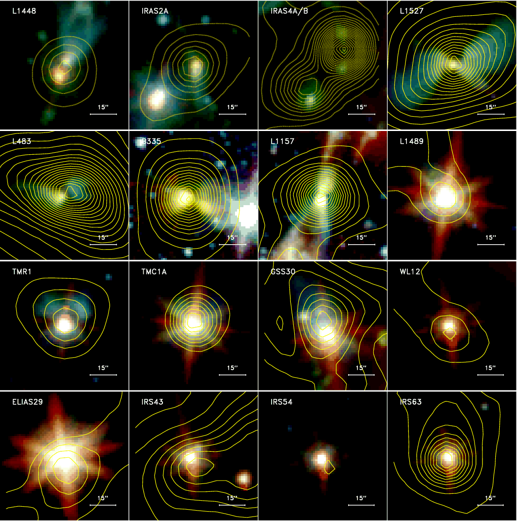
Figure 1:
Spitzer Space Telescope 3.6, 4.5 and 8.0 |
| Open with DEXTER | |
|
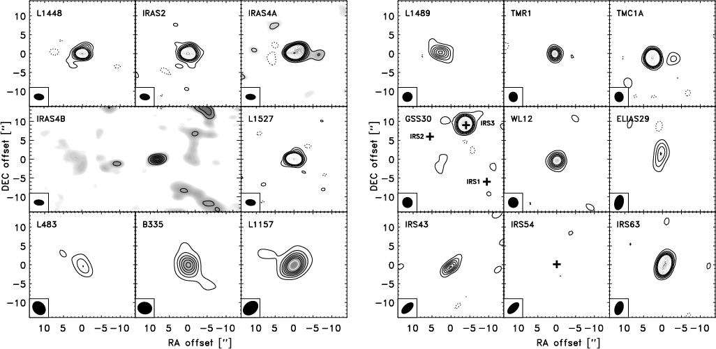
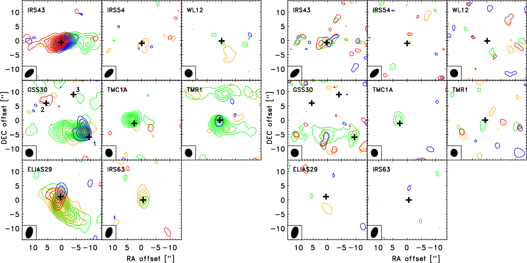
Figure 2:
Overview of the 1.3 mm continuum emission from the Class 0 sources
( left group of panels; see also Jørgensen et al. 2007a) and
1.1 mm continuum emission from the sample of Class I sources
( right group of panels; this paper). Contours are given from 3 |
| Open with DEXTER | |
In addition to the SMA data we collected additional near-infrared data
for each Class I source: Hubble Space Telescope (HST) 1.6 ![]() m
images from the Near Infrared Camera and Multi-Object Spectrometer
(NICMOS) camera were obtained from the HST archive at ESO for TMR1,
TMC1A, IRS 43 and GSS30. The images were registered using existing
near-infrared data (e.g., Barsony et al. 1997). We also include single
pointing HCO+ 3-2 spectra from the James Clerk Maxwell Telescope
(JCMT) archive that were originally presented by Hogerheijde et al. (1997a)
and unpublished observations that were obtained in connection with the
HCO+ 4-3 study by van Kempen et al. (2009). For both Class 0 and I
sources, recalibrated single-dish submillimeter continuum maps
(Fig. 1) were obtained through the JCMT/SCUBA archive
legacy project (Di Francesco et al. 2008).
m
images from the Near Infrared Camera and Multi-Object Spectrometer
(NICMOS) camera were obtained from the HST archive at ESO for TMR1,
TMC1A, IRS 43 and GSS30. The images were registered using existing
near-infrared data (e.g., Barsony et al. 1997). We also include single
pointing HCO+ 3-2 spectra from the James Clerk Maxwell Telescope
(JCMT) archive that were originally presented by Hogerheijde et al. (1997a)
and unpublished observations that were obtained in connection with the
HCO+ 4-3 study by van Kempen et al. (2009). For both Class 0 and I
sources, recalibrated single-dish submillimeter continuum maps
(Fig. 1) were obtained through the JCMT/SCUBA archive
legacy project (Di Francesco et al. 2008).
3 SMA observations of Class I sources
3.1 Observations
The observations of the Class I sources were performed between May
2006 and July 2007 with the Submillimeter Array (SMA) in two
variations of its compact configuration. For all observations, all
8 antennas were available in the array, providing projected
baselines of 9 to 64 k![]() (May 2006 and January 2007 observations) and 9 to
104 k
(May 2006 and January 2007 observations) and 9 to
104 k![]() (June and July 2007 observations). Typically, two sources
were observed per track with the exception of IRS 63 and Elias 29 that
were observed in separate tracks as discussed by Lommen et al. (2008).
(June and July 2007 observations). Typically, two sources
were observed per track with the exception of IRS 63 and Elias 29 that
were observed in separate tracks as discussed by Lommen et al. (2008).
The complex gains were calibrated by observations of 1.5-3 Jy quasars
typically located within 15![]() of the targeted sources once every
20 min. The bandpass was calibrated through observations of strong
quasars and planets at the beginning and end of each track. The quasar
fluxes were bootstrapped through observations of Uranus with a
resulting
of the targeted sources once every
20 min. The bandpass was calibrated through observations of strong
quasars and planets at the beginning and end of each track. The quasar
fluxes were bootstrapped through observations of Uranus with a
resulting ![]() 20% flux calibration uncertainty.
20% flux calibration uncertainty.
The SMA receivers and correlator was configured to observe the lines
of HCN ![]() (265.886444 GHz) and HCO+
(265.886444 GHz) and HCO+ ![]() (267.557648 GHz)
together with the continuum at 1.1 mm: 1 chunk of
512 channels was centered on each of the lines, resulting in a
spectral
resolution of 0.2 MHz or 0.23 km s-1. The remainder of the 2 GHz
bandwidth in each sideband was used to record the continuum.
(267.557648 GHz)
together with the continuum at 1.1 mm: 1 chunk of
512 channels was centered on each of the lines, resulting in a
spectral
resolution of 0.2 MHz or 0.23 km s-1. The remainder of the 2 GHz
bandwidth in each sideband was used to record the continuum.
The initial flagging of the data as well as bandpass, flux and phase/amplitude calibrations were performed in the Mir package (Qi 2008) and subsequent imaging and cleaning in Miriad (Sault et al. 1995). Table 2 summarizes the details of the observations.
Table 2: Log of observations of Class I sources.
3.2 Continuum data overview
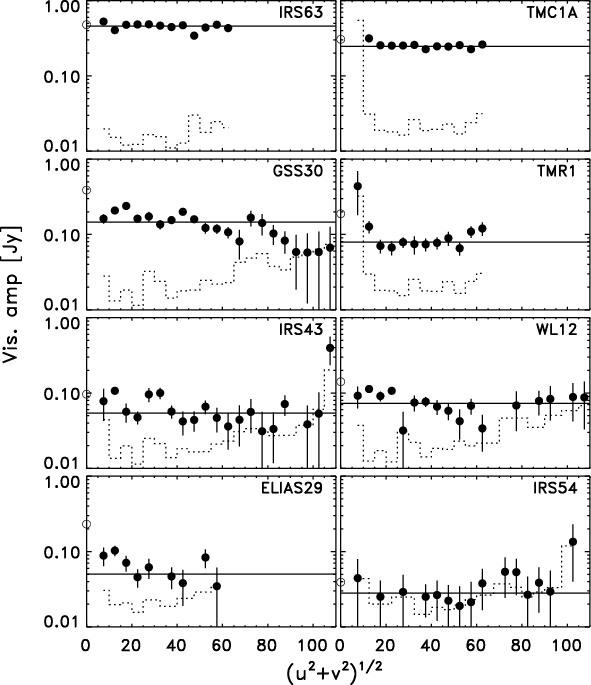
Figure 2 shows the SMA continuum maps of the embedded protostars in the sample at 1.1 mm for the Class I sources as well as the 1.3 mm continuum maps for the Class 0 sources previously presented by Jørgensen et al. (2007a). All sources, except IRS 54, are detected in continuum: one source, TMC1A, shows a fainter secondary component, TMC1A-2 at a separation of 5.5Most of the observed continuum emission has its origin in the inner few hundred AU of the embedded protostars. This is clearly demonstrated in plots of the observed visibilities as function of projected baseline length (Fig. 3). Most sources are roughly consistent with a point, or marginally resolved, source at the resolution of the SMA. These plots are made using circular averages in the (u,v)-plane, i.e., implicitly assume that the emission is spherically symmetric.
To estimate the structure of each source an elliptical Gaussian was
fitted to the continuum flux in the (u,v) plane for baselines longer
than 20 k![]() ,
where the contribution from the larger scale
collapsing envelope becomes negligible and the plots of visibility
amplitude vs. projected baseline length flattens
(Fig. 3). The results are given in
Table 3. The derived fluxes are slightly lower
than the single-dish measurements by Andrews & Williams (2005,2007a)
extrapolated to 1.1 mm assuming optical thin dust with
,
where the contribution from the larger scale
collapsing envelope becomes negligible and the plots of visibility
amplitude vs. projected baseline length flattens
(Fig. 3). The results are given in
Table 3. The derived fluxes are slightly lower
than the single-dish measurements by Andrews & Williams (2005,2007a)
extrapolated to 1.1 mm assuming optical thin dust with
![]() and
and ![]() - but still more than 50% of
the total flux for each source is recovered. This suggests that
although the envelope itself contributes on scales smaller than the
approximately 15
- but still more than 50% of
the total flux for each source is recovered. This suggests that
although the envelope itself contributes on scales smaller than the
approximately 15
![]() of the JCMT beam, the flux from the central
compact component dominates. The sources that show the biggest
discrepancies between the single-dish fluxes and interferometric
fluxes (IRS 63, WL 12, GSS30 and Elias 29) are those that show clear
evidence of extended emission in Fig. 1. The deconvolved
sizes of the continuum sources from the Gaussian fits suggest that
they represent structures with sizes of up to 250-300 AU diameter.
of the JCMT beam, the flux from the central
compact component dominates. The sources that show the biggest
discrepancies between the single-dish fluxes and interferometric
fluxes (IRS 63, WL 12, GSS30 and Elias 29) are those that show clear
evidence of extended emission in Fig. 1. The deconvolved
sizes of the continuum sources from the Gaussian fits suggest that
they represent structures with sizes of up to 250-300 AU diameter.
|
Figure 3: Plot of the continuum flux as function of projected baseline length. The dotted histograms indicate the zero-amplitude signal, i.e., the anticipated signal in the absence of source emission. The open circles indicate the single-dish peak flux [in Jy beam-1] from the JCMT/SCUBA maps toward each source extrapolated to 1.1 mm. |
| Open with DEXTER | |
Table 3: Results of elliptical Gaussian and point source fits to the continuum visibilities for the Class I sources.
3.3 Line data overview
Figure 4 shows an overview of the HCO+ 3-2 spectra toward the continuum positions of each source from the interferometric observations, as well as single-dish spectra from the JCMT archive. The HCO+ 3-2 line profiles vary significantly in strength between different sources, but also relatively between the single-dish and interferometric data. In the single-dish data all sources show HCO+ 3-2 lines with intensities of 1.5-10 K km s-1, but in the interferometer data only 6 of the 9 Class I sources have clearly detected lines. IRS 43 shows the highest intensity and broadest line profile in the HCO+ SMA observations. Interestingly, the interferometric spectra toward TMR1 and TMC1A only probe the blue-shifted emission relative to the single-dish systemic velocity. Figure 5 shows SMA maps of the HCO+ and HCN emission integrated over 4 velocity intervals around the systemic velocity. Again, clear differences are found between the sources. IRS 63 and IRS 43 show red- and blue-shifted emission around the continuum position whereas TMR1, TMC1A and GSS30-IRS1 display emission extended from one side relative to the source position. Toward Elias 29 a complex structure with large-scale extended HCO+ emission from the nearby ridge is seen. For that source material with the most extreme red/blue-shifted velocities around the continuum position trace the Keplerian rotation in the inner envelope/disk (see Lommen et al. 2008).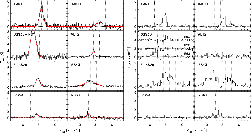
|
Figure 4:
HCO+ 3-2 single-dish spectra from the JCMT archive ( left)
and toward the continuum positions of each source from the SMA
observations ( right). A Gaussian was fitted to each single-dish
spectrum for each source and the centroid velocity as well as
velocities |
| Open with DEXTER | |
|
Figure 5:
Overview of the HCO+ 3-2 ( left) and HCN 3-2
( right) emission from the sample of Class I
sources. The contours (shown in 3 |
| Open with DEXTER | |
4 Analysis of continuum data: disk vs. envelope masses
With large continuum surveys at hand the first step is to disentangle the envelope and disk contributions to the dust continuum emission and from this derive the disk and envelope masses. Ideally fully self-consistent models can be derived for all sources taking into account the full spectral energy distributions as well the interferometric data (e.g., Jørgensen et al. 2005a; Lommen et al. 2008). However, much information can be derived from just simple comparisons of the single-dish and interferometric fluxes.
As discussed by, e.g., Terebey et al. (1993) the continuum emission from a cloud core or circumstellar disk is well approximated by low optical depth in which case the intensity profile is simply found by integrating the temperature and density profile of the core or disk along the line of sight (e.g., Eq. (1) of Terebey et al. 1993). The complication naturally arises that both the density and temperature vary throughout protostellar disks and envelopes. Dust radiative transfer models calculate the dust temperature distribution self-consistently and furthermore produce images at different wavelengths, which can be directly compared to the observations.
In this section we use such dust radiative transfer models to derive the masses of the envelopes and disks around the sample of Class 0 and I protostars. We first explore one-dimensional dust radiative transfer models of protostellar envelopes: we compare the emission from a spherically symmetric envelope around a central source of heating (i.e., protostar) at the scales observed with single-dish telescopes compared to our interferometric observations (Sect. 4.1) and furthermore use the models to establish a direct relationship between the single-dish submillimeter flux and mass of an envelope around a given protostar as function of its luminosity and distance (Sect. 4.2). Finally, we use these results to separate the envelope and disk emission from the envelopes and disks and estimate their masses for each of the objects in our sample (Sects. 4.3 and 4.4).
4.1 Dust radiative transfer models; how much does an envelope contribute to the compact emission?
First, to test the hypothesis that most of the flux in the
interferometric data at baselines of 50 k![]() is in fact from the
central compact component we calculated a set of self-consistent
models for the dust in protostellar envelopes using the
Dusty radiative transfer code (Ivezic et al. 1999). Dusty
solves the temperature profile for a spherically symmetric envelope
around a central source of heating given the power-law envelope density
profile, input spectrum of the central heating source and dust
properties. The code furthermore calculates images at
user-specified wavelengths, which can be compared to observed
images to iteratively place constraints on, e.g., the density
profile. It has previously been used to constrain the physical
structures of the envelopes around a large sample of
deeply embedded protostars (Jørgensen et al. 2002).
is in fact from the
central compact component we calculated a set of self-consistent
models for the dust in protostellar envelopes using the
Dusty radiative transfer code (Ivezic et al. 1999). Dusty
solves the temperature profile for a spherically symmetric envelope
around a central source of heating given the power-law envelope density
profile, input spectrum of the central heating source and dust
properties. The code furthermore calculates images at
user-specified wavelengths, which can be compared to observed
images to iteratively place constraints on, e.g., the density
profile. It has previously been used to constrain the physical
structures of the envelopes around a large sample of
deeply embedded protostars (Jørgensen et al. 2002).
We fixed the effective temperature of the central black-body to 1500 K
mimicking the combined contribution from a low effective temperature
young star and a disk. Since most of this emission is reprocessed
in the larger-scale cold envelope, the exact shape and temperature
of the input spectrum does not affect the distribution and strength
of the emerging submillimeter emission (see also
Shirley et al. 2002; Jørgensen et al. 2002,2005b; Schöier et al. 2002). We
furthermore fixed the outer envelope radius to 8000 AU (typical of
envelopes in clustered regions such as Ophiuchus and Perseus) and
adopted envelope density profiles with
![]() with
p=1.5. Such density profiles are expected for free-falling
envelopes, e.g., within the collapse expansion wave in the inside-out
collapse model of Shu (1977). Detailed models of envelopes of Class
0 and I sources constrained by SCUBA mapping observations find density
profiles with
p=1.5-2.0(e.g., Jørgensen et al. 2002; Shirley et al. 2002; Young et al. 2003). Those models do not
include the contributions from a central disk, which can steepen the
derived density profile index artificially by 0.2-0.5. A power-law
index of 1.5-1.8 for the envelope density profile therefore appears
to be consistent with the envelope structure at these scales. As in
previous work, we adopt the dust opacity law of Ossenkopf & Henning (1994) for
grains with thin ice mantles, coagulated at a density of
with
p=1.5. Such density profiles are expected for free-falling
envelopes, e.g., within the collapse expansion wave in the inside-out
collapse model of Shu (1977). Detailed models of envelopes of Class
0 and I sources constrained by SCUBA mapping observations find density
profiles with
p=1.5-2.0(e.g., Jørgensen et al. 2002; Shirley et al. 2002; Young et al. 2003). Those models do not
include the contributions from a central disk, which can steepen the
derived density profile index artificially by 0.2-0.5. A power-law
index of 1.5-1.8 for the envelope density profile therefore appears
to be consistent with the envelope structure at these scales. As in
previous work, we adopt the dust opacity law of Ossenkopf & Henning (1994) for
grains with thin ice mantles, coagulated at a density of
![]() .
This dust opacity law has
.
This dust opacity law has
![]() cm2 g-1 (dust+gas) and scales
approximately with frequency as
cm2 g-1 (dust+gas) and scales
approximately with frequency as
![]() at
1 mm. Since we for now just deal with the fluxes at submillimeter
wavelengths, the derived masses can be directly rescaled using a
different dust opacity law.
at
1 mm. Since we for now just deal with the fluxes at submillimeter
wavelengths, the derived masses can be directly rescaled using a
different dust opacity law.

|
Figure 6:
Ratio of interferometric fluxes (1.1 mm flux at
50 k |
| Open with DEXTER | |
With these fixed parameters we then calculated a set of dust radiative
transfer models varying the inner radius, luminosity and mass of the
envelope. We tested models with inner radii,
Ri=10, 25, 50,
100, 200 AU, envelope masses between 0.01 and 0.5 ![]() and
luminosities of 1 and 5
and
luminosities of 1 and 5 ![]() .
Together these parameter ranges
cover models representative for the majority of our sources.
.
Together these parameter ranges
cover models representative for the majority of our sources.
For each model, the radiative transfer code calculates the
temperature profile self-consistently as well as images at the
wavelengths of our single-dish and interferometric observations
(850 ![]() m and 1.1 mm, respectively). The images at the wavelength of
our interferometric data were subsequently multiplied by the SMA
primary beam and Fourier transformed, mimicking the interferometric
observations. From these observations we extracted the flux at
baselines of 50 k
m and 1.1 mm, respectively). The images at the wavelength of
our interferometric data were subsequently multiplied by the SMA
primary beam and Fourier transformed, mimicking the interferometric
observations. From these observations we extracted the flux at
baselines of 50 k![]() (3.5
(3.5
![]() diameter) as an estimate of the
contribution to the SMA 1.1 mm flux from the envelope. Likewise,
images at 850
diameter) as an estimate of the
contribution to the SMA 1.1 mm flux from the envelope. Likewise,
images at 850 ![]() m were convolved with the SCUBA beam and the peak
flux in the central beam was extracted as an estimate of its
single-dish 850
m were convolved with the SCUBA beam and the peak
flux in the central beam was extracted as an estimate of its
single-dish 850 ![]() m peak flux.
m peak flux.
Figure 6 shows the ratio of the 1.1 mm interferometric
fluxes at baselines of 50 k![]() and single-dish peak fluxes at
850
and single-dish peak fluxes at
850 ![]() m as function of single-dish peak flux. As shown, the
contribution of the envelope to 1.1 mm emission at baselines of
50 k
m as function of single-dish peak flux. As shown, the
contribution of the envelope to 1.1 mm emission at baselines of
50 k![]() is at most only 4% of the modeled 850
is at most only 4% of the modeled 850 ![]() m peak
flux. If the envelope is steeper,
m peak
flux. If the envelope is steeper,
![]() ,
which seems to
be the steepest envelope structure supported by the modeling of the
single-dish data, the envelope contribution to the 1.1 mm emission at
baselines of 50 k
,
which seems to
be the steepest envelope structure supported by the modeling of the
single-dish data, the envelope contribution to the 1.1 mm emission at
baselines of 50 k![]() increases to 8% of the peak single-dish
flux at 850
increases to 8% of the peak single-dish
flux at 850 ![]() m.
m.
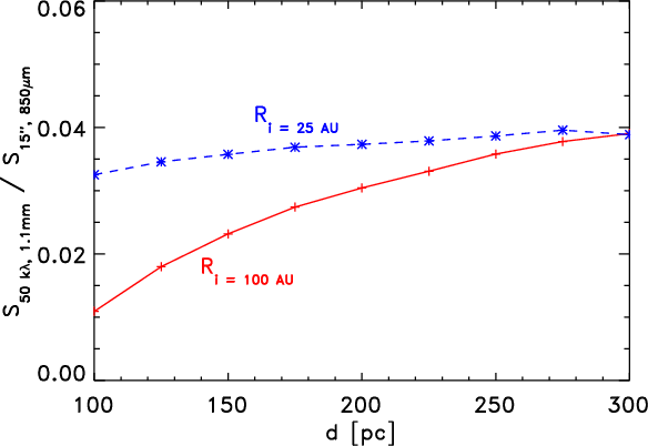
As expected models with large inner radii resolved by the interferometer show less compact flux lowering the ratio of the interferometer-to-single-dish flux. This increase in flux with decreasing inner radius reaches its maximum of 4% for an inner radius of about 25 AU. Material at smaller inner radii is not probed by the existing interferometric observations: this reflects the distribution of mass in the power-law envelope ensuring that most mass is at large scales, or that most of the dust continuum emission is due to mass located at the typical size scale probed by the interferometer.
Using these results we can estimate an upper limit to the envelope
contribution at 50 k![]() for the observed sources by taking 4%
of the 850
for the observed sources by taking 4%
of the 850 ![]() m JCMT peak flux and comparing that directly to the
observed 1.1 mm interferometric flux at 50 k
m JCMT peak flux and comparing that directly to the
observed 1.1 mm interferometric flux at 50 k![]() :
the ratio
between these two numbers then gives the relative envelope
contribution to the 1.1 mm interferometric data. This comparison
confirms that the 1.1 mm SMA measurements of the Class I sources
(Table 3) predominantly contain emission from the
central disk: in median, 87% of the observed interferometer flux is
from the disk, as also suggested by their flat visibility amplitudes
as function of projected baseline length in
Fig. 3. For comparison, the Class 0 sources have a
median disk contribution of 68% of their observed interferometer
flux. The results in Fig. 6 are shown for a distance
of 125 pc. The ratio between the interferometer and single-dish peak
flux measures the relative surface brightnesses on the spatial
scales probed by each and does not change significantly when the
distance increases - as long as the inner envelope cavity is not
large enough to be resolved (Fig. 7).
:
the ratio
between these two numbers then gives the relative envelope
contribution to the 1.1 mm interferometric data. This comparison
confirms that the 1.1 mm SMA measurements of the Class I sources
(Table 3) predominantly contain emission from the
central disk: in median, 87% of the observed interferometer flux is
from the disk, as also suggested by their flat visibility amplitudes
as function of projected baseline length in
Fig. 3. For comparison, the Class 0 sources have a
median disk contribution of 68% of their observed interferometer
flux. The results in Fig. 6 are shown for a distance
of 125 pc. The ratio between the interferometer and single-dish peak
flux measures the relative surface brightnesses on the spatial
scales probed by each and does not change significantly when the
distance increases - as long as the inner envelope cavity is not
large enough to be resolved (Fig. 7).
|
Figure 7:
Ratio between the interferometer flux at 1.1 mm and
single-dish beam peak flux at 850 |
| Open with DEXTER | |
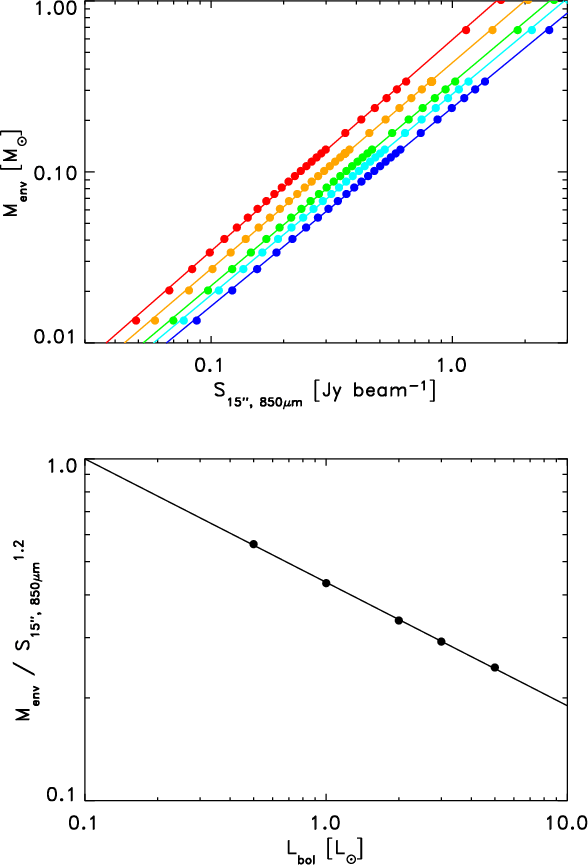
|
Figure 8:
Results of dust radiative transfer calculations for simple
envelope models at d=125 pc. Upper: the relation between
envelope mass and peak flux in the JCMT beam for envelope models
with 0.5, 1, 2, 3 and 5 |
| Open with DEXTER | |
4.2 Calibration of envelope mass - continuum flux relation
With a separation of the envelope and disk contribution to the single-dish and interferometric observations, the next task is to derive masses from each component using the observed fluxes. For prestellar cores it is usually a good approximation to assume that their dust is optically thin and isothermal with a temperature of 10-15 K and from that estimate the mass of the core from single-dish observations of their submillimeter continuum fluxes. However, an envelope with an internal heating source, such as a central protostar, will have a distribution of temperatures - which will strongly depend on the source luminosity.
A way to circumvent these problems is again to use the results
from the detailed dust radiative transfer models:
Fig. 8 compares the relations between the envelope
mass, peak flux and luminosity for the protostellar envelopes
determined from the radiative transfer modeling. As shown these dust
radiative transfer models give rise to simple power-law relationships
between the envelope mass and observables which can be expressed as:
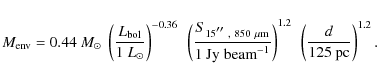
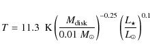
Together with the luminosity, the above expression makes it possible to evaluate the mass of each protostellar envelope from its peak flux only - once the contribution from the disk emission to the single-dish flux has been subtracted (see also Sect. 4.3). This relation is particularly useful in crowded regions where it is possible to estimate the peak flux of a given source, but where it is difficult to evaluate its outer radius and thus its extended flux due to confusion. The luminosity can either be derived from the full spectral energy distribution of each source or by using the empirical correlation between source internal luminosity and 70
These results are generally in good agreement with the models
discussed by Terebey et al. (1993): they find a relationship between the
flux and luminosity and distance which for a given envelope mass
scales roughly as
![]() compared to our results
which for a given envelope mass are equivalent to
compared to our results
which for a given envelope mass are equivalent to
![]() .
The different slope with respect to distance is caused by
the slightly flatter density profile predicted by the Terebey et al. (1984)
model: for a power-law envelope similar to ours, Terebey et al. (1993) find
that
.
The different slope with respect to distance is caused by
the slightly flatter density profile predicted by the Terebey et al. (1984)
model: for a power-law envelope similar to ours, Terebey et al. (1993) find
that
![]() .
The remaining difference in the exponent of
this relation as well as the difference in the exponents for the
luminosity is caused by the envelopes being slightly optically thick
to their own radiation which increases the temperature (and thus
emission) on small scales and causes the underlying temperature
profile to depart from the single power-law applicable for an envelope
fully optically thin to its own radiation.
.
The remaining difference in the exponent of
this relation as well as the difference in the exponents for the
luminosity is caused by the envelopes being slightly optically thick
to their own radiation which increases the temperature (and thus
emission) on small scales and causes the underlying temperature
profile to depart from the single power-law applicable for an envelope
fully optically thin to its own radiation.
The derived expressions are particularly useful for interpreting large
samples of sources detected, e.g., through the large-scale
submillimeter maps provided by ongoing and upcoming surveys with
bolometer arrays such as LABOCA and SCUBA 2. One of the main goals of
those surveys are naturally to determine core masses and this is often
done using single isothermal cores with two temperatures: one for
cores with and one without embedded protostellar sources
(e.g., Hatchell & Fuller 2008; Enoch et al. 2007). However, with
Eq. (1) we can take the dependence of the source
submillimeter flux on the luminosity into account: according to
Eq. (1) a factor 2.3 decrease in mass is expected due
to the increase of the luminosity by a factor 10 for the same peak
flux - or put in another way: if the mass for a 1 ![]() core is
derived using a temperature of 15 K, that for a 10
core is
derived using a temperature of 15 K, that for a 10 ![]() protostellar core should adopt a temperature of 23.5 K. Assuming a
similar temperature for all protostellar cores would therefore lead to
a mass-luminosity relation,
protostellar core should adopt a temperature of 23.5 K. Assuming a
similar temperature for all protostellar cores would therefore lead to
a mass-luminosity relation,
![]() .
This is slightly steeper
but close to the relation found by Hatchell et al. (2007) with
.
This is slightly steeper
but close to the relation found by Hatchell et al. (2007) with
![]() with an uncertainty of
with an uncertainty of ![]() 0.36 in the power-law index of
the observationally derived relation.
0.36 in the power-law index of
the observationally derived relation.
4.3 Determining envelope and disk masses from continuum measurements
With the resuts from the previous section we can now compare the
derived compact and single-dish fluxes across the sample. The Class 0
and I sources were not observed at exactly the same wavelengths at the
SMA. The Class 0 sources were observed at 1.3 mm (230 GHz) and 0.8 mm
(345 GHz) whereas the Class I sources discussed here were observed at
1.1 mm (270 GHz). Class 0 and I sources have been observed at
850 ![]() m with SCUBA on the JCMT. To take this difference into
account we interpolate the Class 0 point source fluxes estimated on
baselines longer than 40 k
m with SCUBA on the JCMT. To take this difference into
account we interpolate the Class 0 point source fluxes estimated on
baselines longer than 40 k![]() from Jørgensen et al. (2007a) using the
derived spectral slope of 2.5 from that paper, i.e., less steep than
for the envelope. With this correction the fluxes of each source at
similar angular scales are compared directly
(Fig. 9).
from Jørgensen et al. (2007a) using the
derived spectral slope of 2.5 from that paper, i.e., less steep than
for the envelope. With this correction the fluxes of each source at
similar angular scales are compared directly
(Fig. 9).
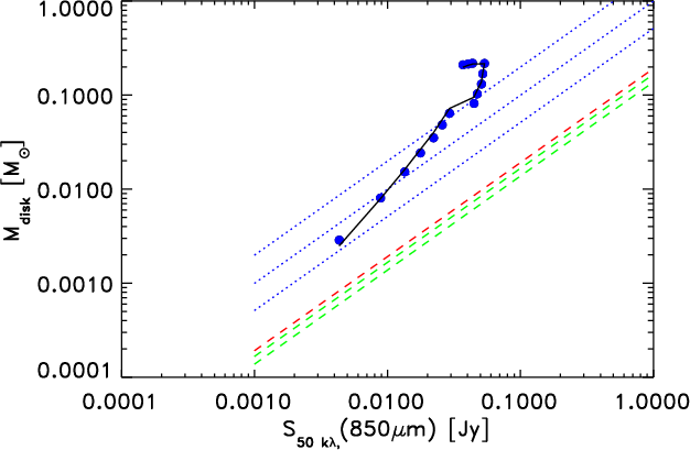
|
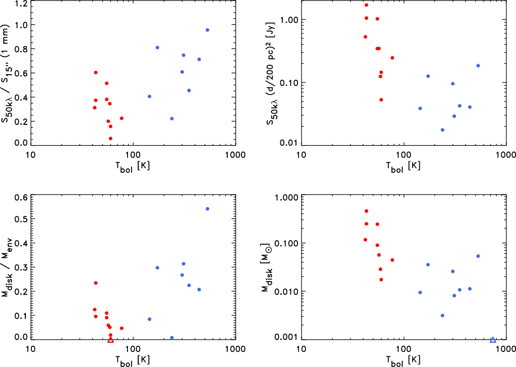
Figure 9:
Single-dish and interferometer fluxes as well as disk and
envelope masses as function of source bolometric temperatures.
The upper panels show the ratios of the interferometer
and single-dish flux ( left) and the interferometer flux
( right) and the lower panels the ratio of the disk and
envelope mass ( left) and disk mass ( right).
Class 0 sources are shown with red symbols and Class I with blue
symbols. In the lower left panel, L483 (Class 0 source with
envelope-only emission; see discussion in text) is shown with the
red triangle. In the lower right panel, IRS 54 (Class I source with
no detected interferometric or single dish emission) is shown with a
3 |
| Open with DEXTER | |
To estimate the masses of both components, a few more steps are
required: both the envelope and disk contribute to the observed
emission in both the single-dish and interferometer beams. However,
with the above results we can quantify the maximum contribution from
the envelope on the 1.1 mm interferometric flux at 50 k![]() as no
more than about 4% of the envelope single-dish peak flux at
850
as no
more than about 4% of the envelope single-dish peak flux at
850 ![]() m. Using this upper limit, we can write the two equations
with the envelope flux at 850
m. Using this upper limit, we can write the two equations
with the envelope flux at 850 ![]() m,
m,
![]() ,
and disk flux at
1.1 mm,
,
and disk flux at
1.1 mm,
![]() as two unknowns that can easily be solved for:
as two unknowns that can easily be solved for:
In these equations ![]() is the spectral index
is the spectral index![]() of the dust continuum emission at
millimeter wavelengths in the disks found to be
of the dust continuum emission at
millimeter wavelengths in the disks found to be ![]() 2.5 from the observations of the Class 0
sources in our sample (Jørgensen et al. 2007a). c is the fraction of the envelope
850
2.5 from the observations of the Class 0
sources in our sample (Jørgensen et al. 2007a). c is the fraction of the envelope
850 ![]() m single-dish peak flux observed at 1.1 mm by the
interferometer at 50 k
m single-dish peak flux observed at 1.1 mm by the
interferometer at 50 k![]() .
For this discussion we adopt the
upper limit to c=0.04 from the above discussion for
p=1.5. We note that this contribution generally is small enough
that the direct measurement by the interferometer is a good first
estimate of the actual compact flux not associated with the infalling
(
.
For this discussion we adopt the
upper limit to c=0.04 from the above discussion for
p=1.5. We note that this contribution generally is small enough
that the direct measurement by the interferometer is a good first
estimate of the actual compact flux not associated with the infalling
(
![]() )
envelope.
)
envelope.
To derive envelope masses, a few additional effects need to be taken into account here: as shown above the envelope masses scale with distance as d1.2 for a fixed peak flux, whereas the disk masses (largely unresolved) are expected to scale as d2. In addition, since the submillimeter continuum emission measures the dust mass weighted by temperature, the derived envelope masses are found to depend on the luminosity (see, Eq. (1)). Taking this into account, however, it is possible to directly estimate the masses of the envelopes from the observed fluxes once the contribution from the disk has been estimated through Eqs. (2) and (3) (Table 4). For the disk masses we assume that the dust continuum emission is optically thin and coming from an isothermal disk with a temperature of 30 K and a dust opacity at 1.1 mm similar to that of the dust in the protostellar envelopes. We return a discussion of these assumptions in Sect. 6.1
Table 4: Envelope and disk masses for the full sample of Class 0 and I sources.
4.4 Resulting disk and envelope masses
Figure 9 compares the interferometric and single-dish
fluxes scaled to 1.1 mm as well as disk and envelope masses for all
the sources in our sample. As expected the deeply embedded, Class 0,
protostars have larger fluxes in the single-dish relative to the
smaller interferometric beam, reflected in a lower
![]() ratio (upper left panel of
Fig. 9). A similar effect was noted by
Ward-Thompson (2007) who compared interferometric and single-dish
fluxes at 850
ratio (upper left panel of
Fig. 9). A similar effect was noted by
Ward-Thompson (2007) who compared interferometric and single-dish
fluxes at 850 ![]() m from literature studies of a sample of 9 YSOs (6 Class 0, 2 Class I and
1 Class II sources). Taken by itself this can
naturally reflect one or two effects: (i) the envelope masses
for these sources are larger also resulting in their redder SEDs or;
(ii) the disk masses are smaller for the more deeply embedded
protostars (e.g., if significant disk growth occurs from the Class 0
through I stages). The interferometric fluxes do not show such an
increase going from the Class 0 to I stages, however (upper right
panel of Fig. 9). This argues against a
significant increase in disk masses being the explanation.
m from literature studies of a sample of 9 YSOs (6 Class 0, 2 Class I and
1 Class II sources). Taken by itself this can
naturally reflect one or two effects: (i) the envelope masses
for these sources are larger also resulting in their redder SEDs or;
(ii) the disk masses are smaller for the more deeply embedded
protostars (e.g., if significant disk growth occurs from the Class 0
through I stages). The interferometric fluxes do not show such an
increase going from the Class 0 to I stages, however (upper right
panel of Fig. 9). This argues against a
significant increase in disk masses being the explanation.
The lower panels of Fig. 9 compare the
envelope and disk masses for all the sources in the Class 0 and I
samples as a function of bolometric temperature. Again, the
disk/envelope mass ratio is seen to be lower for the more deeply
embedded Class 0 protostars reflecting their higher envelope masses at
comparable disk masses as those in the Class I stages (lower left
panel of Fig. 9). Typically the Class 0
protostars have disks that contain about 1-10% of the total
disk+envelope mass whereas the disks around the Class I sources
contain 20-60% of the disk+envelope mass. In both stages most of the
derived disk masses are in the range of ![]() 0.01 to 0.1
0.01 to 0.1 ![]() with the median Class 0 disk mass of 0.089
with the median Class 0 disk mass of 0.089 ![]() and the median
Class I disk mass of 0.011
and the median
Class I disk mass of 0.011 ![]() .
The drop in envelope masses from
the Class 0 to I stages and the relatively low disk masses, suggests
that a significant fraction of the mass of the central star is
attained already during the most deeply embedded stages.
.
The drop in envelope masses from
the Class 0 to I stages and the relatively low disk masses, suggests
that a significant fraction of the mass of the central star is
attained already during the most deeply embedded stages.
The results above do not show evidence for an increasing disk mass
going from the Class 0 sources to the Class I sources in the observed
samples. Thus, either the disks build up rapidly during the early,
deeply embedded stages or their physical properties (e.g., grain
properties, temperatures) are significantly different than those in
more evolved stages. Andrews & Williams (2005,2007b) examined the relation
between the disk masses for a large sample of Class I and II sources
in Ophiuchus and Taurus and found evidence for a decrease of the disk
masses by a factor 3 between these evolutionary stages from a median
disk mass of 0.015 ![]() to 0.005
to 0.005 ![]() .
.
Although most sources show compact emission, there are exceptions: the
interferometric flux of the L483 Class 0 source is found to be
consistent with envelope-only emission and does not require a central
compact source. This is similar to the conclusion of Jørgensen (2004)
who modeled 3 mm continuum emission of the source from OVRO
observations. It is also in agreement with the measured spectral slope
of the SMA continuum flux between 1.3 and 0.8 mm (Jørgensen et al. 2007a),
which shows an index of ![]() 4, consistent with optically thin
dust in a larger scale envelope, contrasting the other Class 0 sources
in the sample which have lower spectral indices in the range of 2-3
(Fig. 3 of Jørgensen et al. 2007a). It is puzzling that no direct
evidence of a dust disk is seen for this source, given that it has a
well-established protostellar outflow - which even seems to be in the
process of actively dispersing the envelope. This may be a case,
however, where we overestimate the contribution by the envelope on the
longest baselines from the radiative transfer models. If the envelope,
for example, has a larger flattened inner region or cavity, the
envelope contribution on the longer baselines would be smaller and a
central circumstellar disk required to explain the submillimeter
emission. The mass of this disk would in that case be
4, consistent with optically thin
dust in a larger scale envelope, contrasting the other Class 0 sources
in the sample which have lower spectral indices in the range of 2-3
(Fig. 3 of Jørgensen et al. 2007a). It is puzzling that no direct
evidence of a dust disk is seen for this source, given that it has a
well-established protostellar outflow - which even seems to be in the
process of actively dispersing the envelope. This may be a case,
however, where we overestimate the contribution by the envelope on the
longest baselines from the radiative transfer models. If the envelope,
for example, has a larger flattened inner region or cavity, the
envelope contribution on the longer baselines would be smaller and a
central circumstellar disk required to explain the submillimeter
emission. The mass of this disk would in that case be
![]() 0.01
0.01 ![]() - derived from the long baseline
interferometric data without taking the larger scale envelope
contribution into account (Jørgensen et al. 2007a).
- derived from the long baseline
interferometric data without taking the larger scale envelope
contribution into account (Jørgensen et al. 2007a).
In a recent study Girart et al. (2009) modeled SMA continuum data for the
Class 0 protostellar binary L723 and likewise found that a disk was
not required to explain the compact continuum emission. Scaling their
observed flux at 1.35 mm from the SMA at baselines of about
50 k![]() to our reference wavelength at 1.1 mm gives a flux of
about 35 mJy - or about 3-4% of the observed SCUBA peak flux of
1.1 Jy beam-1 from the JCMT/SCUBA legacy catalog
(Di Francesco et al. 2008). Within our framework this fraction is exactly
what is expected for envelope only contribution at these baselines,
and in agreement with the interpretation by Girart et al. (2009) that no
disk is required to explain the SMA continuum observations, but with a
note that if the envelope would have an inner flattened region, an
additional central dust component would be required - again with a
typical mass
to our reference wavelength at 1.1 mm gives a flux of
about 35 mJy - or about 3-4% of the observed SCUBA peak flux of
1.1 Jy beam-1 from the JCMT/SCUBA legacy catalog
(Di Francesco et al. 2008). Within our framework this fraction is exactly
what is expected for envelope only contribution at these baselines,
and in agreement with the interpretation by Girart et al. (2009) that no
disk is required to explain the SMA continuum observations, but with a
note that if the envelope would have an inner flattened region, an
additional central dust component would be required - again with a
typical mass ![]() a few
a few ![]() 0.01
0.01 ![]() .
.
5 Analysis of line data: stellar masses
In the previous section masses were determined for two of the three YSO components - their disks and envelopes. The resolved line observations obtained for the Class I sources provide information about the dynamical structure of their inner envelopes and disks and thereby a handle on the mass of the third component, the central star.
As mentioned above, significant differences exist between the
components traced by the line observations for the different sources
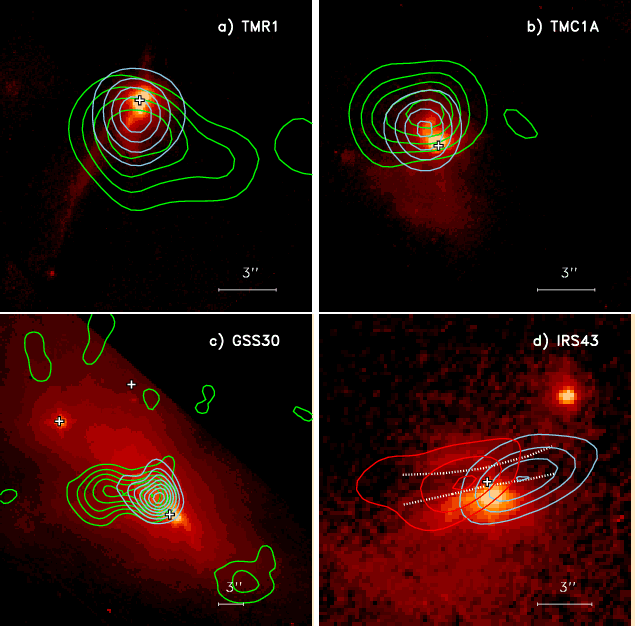
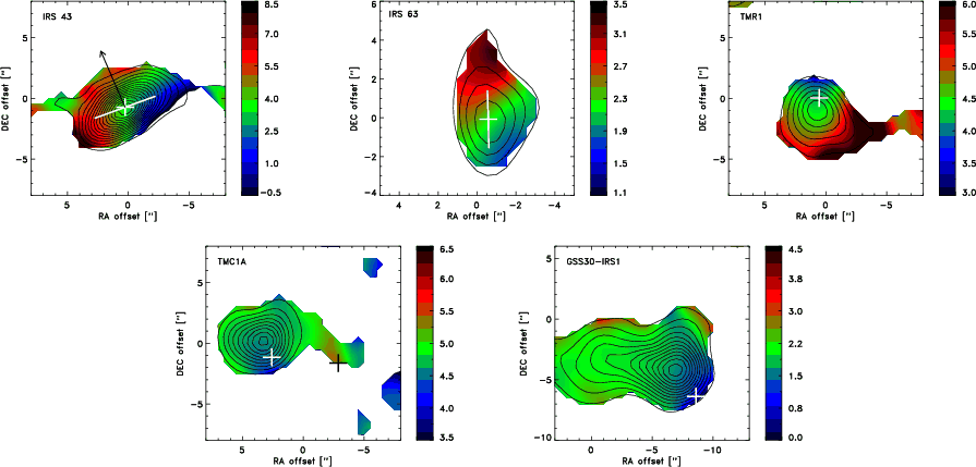
in the sample. Figure 10 compares the near-infrared
1.6 ![]() m images to the HCO+ emission in TMR1, TMC1A, GSS30-IRS1
and IRS 43. The first three of these sources show a clear alignment
with the near-infrared scattering nebulosities whereas the fourth,
IRS 43, shows the HCO+ (and also HCN) emission aligned with the
dark lane across the source. Likewise, in the first order moment
(velocity) maps (Fig. 11), TMR1, TMC1A and GSS30 show
significantly different morphologies from IRS 43 and IRS 63: the
former sources show evidence of blue-shifted emission over most of
their maps, with velocities decreasing toward the systemic velocities
at the largest distances. In contrast IRS 43, in particular, shows a
clear large-scale velocity gradient relative to the continuum peak
position and systemic velocity, potentially indicative of rotation as
also inferred for IRS 63, Elias 29 (Lommen et al. 2008) and L1489-IRS
(Brinch et al. 2007). In the following we focus on the use of
HCO+ as a tracer of rotation in these sources and include a small
discussion of the sources showing outflow cavities and the
limitations of HCO+ as a tracer in Appendix A. Some
details about the individual Class I sources are given in
Appendix B.
m images to the HCO+ emission in TMR1, TMC1A, GSS30-IRS1
and IRS 43. The first three of these sources show a clear alignment
with the near-infrared scattering nebulosities whereas the fourth,
IRS 43, shows the HCO+ (and also HCN) emission aligned with the
dark lane across the source. Likewise, in the first order moment
(velocity) maps (Fig. 11), TMR1, TMC1A and GSS30 show
significantly different morphologies from IRS 43 and IRS 63: the
former sources show evidence of blue-shifted emission over most of
their maps, with velocities decreasing toward the systemic velocities
at the largest distances. In contrast IRS 43, in particular, shows a
clear large-scale velocity gradient relative to the continuum peak
position and systemic velocity, potentially indicative of rotation as
also inferred for IRS 63, Elias 29 (Lommen et al. 2008) and L1489-IRS
(Brinch et al. 2007). In the following we focus on the use of
HCO+ as a tracer of rotation in these sources and include a small
discussion of the sources showing outflow cavities and the
limitations of HCO+ as a tracer in Appendix A. Some
details about the individual Class I sources are given in
Appendix B.
|
Figure 10:
Archive 1.6 |
| Open with DEXTER | |
|
Figure 11: Moment one (velocity) maps of the HCO+ emission for IRS 43, IRS 63, TMR1, TMC1A and GSS30-IRS1. In all panels the plus-signs indicate the location of the continuum positions (for GSS30-IRS1 the near-/mid-infrared source). In the IRS 43 and IRS 63 panels the white line shows the direction of the continuum structure. In the IRS 43 panel, the black arrow furthermore shows the direction of the embedded near-IR Herbig-Haro objects (Grosso et al. 2001) and thermal jet (Girart et al. 2000). |
| Open with DEXTER | |
5.1 Keplerian rotation and stellar mass in IRS 43
Four sources in our sample, IRS 43, IRS 63 and Elias 29 (Fig. 5) as well as L1489-IRS (Brinch et al. 2007), show elongated HCO+ emission stretching across the location of the YSO. As discussed by Brinch et al. (2007) and Lommen et al. (2008) the velocity gradients toward L1489-IRS, IRS 63 and Elias 29 can be interpreted as having their origin in the inner envelope/circumstellar disk around each source. A number of effects point toward this also being the case for IRS 43:- 1.
- both HCN and HCO+ show an elongated structure with a large scale velocity gradient around the continuum peak/systemic velocity;
- 2.
- a Gaussian fit to the continuum data in the (u,v) plane shows
a structure which is elongated in the same direction with a position
angle of -70
 (measured from north toward east): its
deconvolved major axis is about 2
(measured from north toward east): its
deconvolved major axis is about 2
 (280 AU) and its minor axis
about a tenth of an arcsecond, consistent with emission from a
disk seen at a high inclination angle, close to edge-on.
(280 AU) and its minor axis
about a tenth of an arcsecond, consistent with emission from a
disk seen at a high inclination angle, close to edge-on.
- 3.
- The direction of the Herbig-Haro objects (Grosso et al. 2001) and
proposed radio thermal jet (Girart et al. 2000) are with a position
angle of 20-25,
perpendicular to this extended structure
(Figs. 11 and B.1).
|
Figure 12:
Position-velocity (PV) diagram for the HCO+ emission in
IRS 43 directly from the image-plane ( upper panel) and from fitting
the individual channels in the (u,v)-plane ( lower panel). The
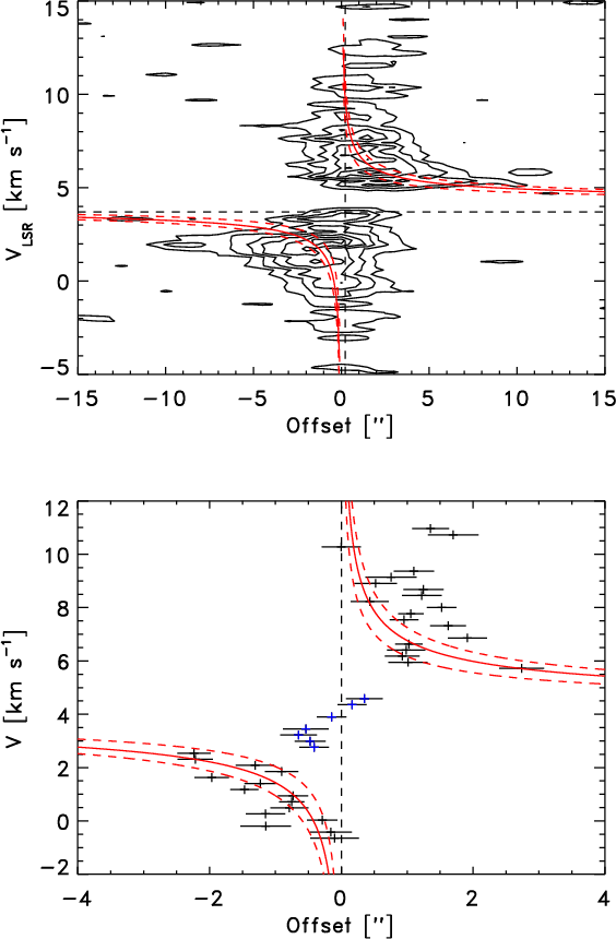
PV diagram has been measured along the major axis of the HCO+ emission at a position angle of -70 |
| Open with DEXTER | |
The extent of the HCO+ emission (![]()
![]() )
suggests that its
origin is not purely in the central disk, but also the inner regions
of the rotating envelope (
)
suggests that its
origin is not purely in the central disk, but also the inner regions
of the rotating envelope (
![]() AU). This is further
supported by the comparison between the single-dish spectrum and a
spectrum extracted from the interferometric data integrated over the
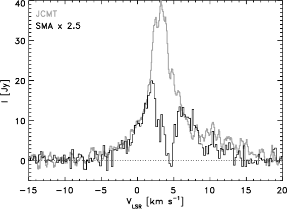
extent of the JCMT single-dish beam (Fig. 13). About 40% of the single-dish flux is recovered by the interferometer,
suggesting the presence of some extended emission resolved out by the
interferometer - although this fraction is significantly less than
typically seen, e.g., in the more deeply embedded Class 0 protostars
(e.g., Jørgensen et al. 2007a).
AU). This is further
supported by the comparison between the single-dish spectrum and a
spectrum extracted from the interferometric data integrated over the
extent of the JCMT single-dish beam (Fig. 13). About 40% of the single-dish flux is recovered by the interferometer,
suggesting the presence of some extended emission resolved out by the
interferometer - although this fraction is significantly less than
typically seen, e.g., in the more deeply embedded Class 0 protostars
(e.g., Jørgensen et al. 2007a).
To derive the mass of the central object a position-velocity curve is
extracted by fitting the position of the peak emission for each
channel in the (u,v)-plane at baselines larger than 20 k![]() and projecting this on the major axis of the HCO+ emission (right
panel, Fig. 12). To this curve, a
and projecting this on the major axis of the HCO+ emission (right
panel, Fig. 12). To this curve, a ![]() -fit is
performed with a straightforward Keplerian rotation curve with two
free parameters, the systemic velocity and central mass. A best fit is
obtained for a central mass of 1.0
-fit is
performed with a straightforward Keplerian rotation curve with two
free parameters, the systemic velocity and central mass. A best fit is
obtained for a central mass of 1.0 ![]() (2
(2![]() confidence
levels of
confidence
levels of ![]() 0.2
0.2 ![]() )
and a systemic velocity of
4.1 km s-1. This mass estimate is of the ``enclosed'' mass within the
resolution of the interferometer, but since it is significantly higher
than the best estimate of the envelope and disk masses of 0.026 and
0.0081
)
and a systemic velocity of
4.1 km s-1. This mass estimate is of the ``enclosed'' mass within the
resolution of the interferometer, but since it is significantly higher
than the best estimate of the envelope and disk masses of 0.026 and
0.0081 ![]() respectively (see Sect. 4), it is
likely close to the total mass of the central star. This is also a
lower limit since it is not corrected for inclination, but given the
small minor axis relative to the major axis from the Gaussian fit to
continuum emission, it is not unreasonable to assign a high
inclination angle corresponding to an edge-on disk.
respectively (see Sect. 4), it is
likely close to the total mass of the central star. This is also a
lower limit since it is not corrected for inclination, but given the
small minor axis relative to the major axis from the Gaussian fit to
continuum emission, it is not unreasonable to assign a high
inclination angle corresponding to an edge-on disk.
In summary, we detect signatures of Keplerian rotation in the
HCO+ 3-2 emission for 4 Class I sources allowing direct
determinations of their central stellar masses, which range from
about 0.3 to 2.5 ![]() .
As discussed in Appendix A.2, the
100 AU scales of embedded protostars can only be traced with HCO+ 3-2 in sources with envelope masses less than about 0.1
.
As discussed in Appendix A.2, the
100 AU scales of embedded protostars can only be traced with HCO+ 3-2 in sources with envelope masses less than about 0.1 ![]() ,
however. Future high sensitivity ALMA observations will be required
to observe more optically thin isotopes, to determine the dynamical
structure of the more deeply protostars.
,
however. Future high sensitivity ALMA observations will be required
to observe more optically thin isotopes, to determine the dynamical
structure of the more deeply protostars.
6 Discussion
6.1 Effects of assumed dust properties and temperatures on disk masses
As in most other
studies in the literature, two assumptions in our study are that the disk can be characterized by a
uniform temperature and by a single unchanging dust opacity law
throughout its extent and evolution. Both these assumptions may
affect the systematic trends observed in the data: for the
temperature an increase in luminosity increases the mass-weighted
temperature of the disk, while the shielding by the disk itself will
lead to a lower mass weighted temperature with increasing mass. As an
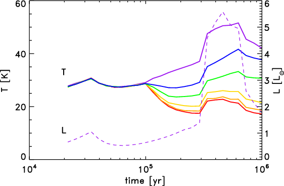
example, Fig. 14 compares the temporal evolution of
the temperature at a radius of 200 AU between rays through the model
with different inclinations with respect to the disk plane in the
simulation of Visser et al. (2009). Also shown is the evolution of the
luminosity in the simulations. Early in the evolution, before the disk
is formed, the temperature tracks the luminosity changes closely, but
as the disk forms (at about 105 years) the temperature at
inclinations directed through the disk drops sharply, even though the
luminosity continues to increase. The strong increase in total
luminosity at about
![]() years is directly reflected in the
temperature profiles.
years is directly reflected in the
temperature profiles.
|
Figure 13: IRS 43: comparison between HCO+ 3-2 spectrum from the SMA data integrated over the single-dish beam and JCMT observations. The interferometric spectrum has been scaled by a factor 2.5. |
| Open with DEXTER | |
|
Figure 14:
Temporal evolution of the temperature and luminosity in the
simulation of Visser et al. (2009). The solid lines shows the temperature at 200 AU along rays inclined with 0, 5, 10, 15, 20 and 90 |
| Open with DEXTER | |
Figure 15 compares the relationships between (sub)millimeter
flux and disk mass adopted by Terebey et al. (1993), Andrews & Williams (2007b) and
Jørgensen et al. (2007a) to the relationship predicted by the radiative
transfer modeling of the collapse simulation from Visser et al. (2009): it
is clearly seen that the models require a steeper relationship between
the submillimeter flux and disk mass than what is obtained with a
single constant temperature: to calculate the disk mass from the
submillimeter flux in the model, one would need a temperature scaling as:
as shown with the solid line in Fig. 15 - i.e., an increasing temperature with increasing luminosity (and thus heating) and a decreasing temperature with increasing disk mass (and thus shielding at a given radius). Although the variations in the temperature with disk mass and stellar luminosity are slow, they still introduce a systematic gradient in the derived disk masses by up to a factor of 4 through the evolution of the embedded stages of the YSOs. It thus appears that the disk masses in the later stages relative to the early stages can be underestimated by about this factor - solely due to the evolution of the protostellar system. This may explain the slightly higher masses for the Class 0 sources in Fig. 9.
|
Figure 15:
Relationship between disk mass and 850 |
| Open with DEXTER | |
Figure 16 compares the derived disk masses to
bolometric temperature as well as the ratio of the source luminosity
over the envelope mass,
![]() .
The latter ratio is
an alternative evolutionary tracer, increasing with time as long as
the YSO luminosity is dominated by accretion and the stellar mass (and
luminosity) increases, whereas the envelope dissipates and its mass
decreases. In this figure the Class 0 disk masses are decreased by a
factor of 2 and the Class I disk masses increased by a factor of 2 to
simulate the temperature effect discussed above. With this correction,
the Class 0 and I disk masses are roughly constant with a median mass
of about 0.04
.
The latter ratio is
an alternative evolutionary tracer, increasing with time as long as
the YSO luminosity is dominated by accretion and the stellar mass (and
luminosity) increases, whereas the envelope dissipates and its mass
decreases. In this figure the Class 0 disk masses are decreased by a
factor of 2 and the Class I disk masses increased by a factor of 2 to
simulate the temperature effect discussed above. With this correction,
the Class 0 and I disk masses are roughly constant with a median mass
of about 0.04 ![]() for the full sample.
for the full sample.
The assumption of a constant unchanging dust opacity law similar to
the large-scale envelope dust may also be wrong: in particular, grain
growth may increase the dust opacity at submillimeter wavelengths
leading to a lower derived disk mass for a given interferometric
flux. That something like this may be going on is hinted by the
observation that the compact components around the Class 0 sources
show spectral slopes, ![]() ,
of the emission
,
of the emission
![]() ,
at 230 and 345 GHz in the range 2-3
(Jørgensen et al. 2007a). This suggests that the disks are either optically
thick or have significantly different dust opacities than standard ISM
dust. As discussed in Jørgensen et al., the disk masses
implied for the Class 0 objects suggest that only the most massive
ones may be marginally optically thick. Resolved observations at
multiple wavelengths and measurements of their sizes are required to
address this. On the other hand, the low spectral indices confirm that
the compact components around the Class 0 sources are not associated
with the larger scale envelopes for which an
,
at 230 and 345 GHz in the range 2-3
(Jørgensen et al. 2007a). This suggests that the disks are either optically
thick or have significantly different dust opacities than standard ISM
dust. As discussed in Jørgensen et al., the disk masses
implied for the Class 0 objects suggest that only the most massive
ones may be marginally optically thick. Resolved observations at
multiple wavelengths and measurements of their sizes are required to
address this. On the other hand, the low spectral indices confirm that
the compact components around the Class 0 sources are not associated
with the larger scale envelopes for which an ![]() of 3.5-4 is
expected.
of 3.5-4 is
expected.
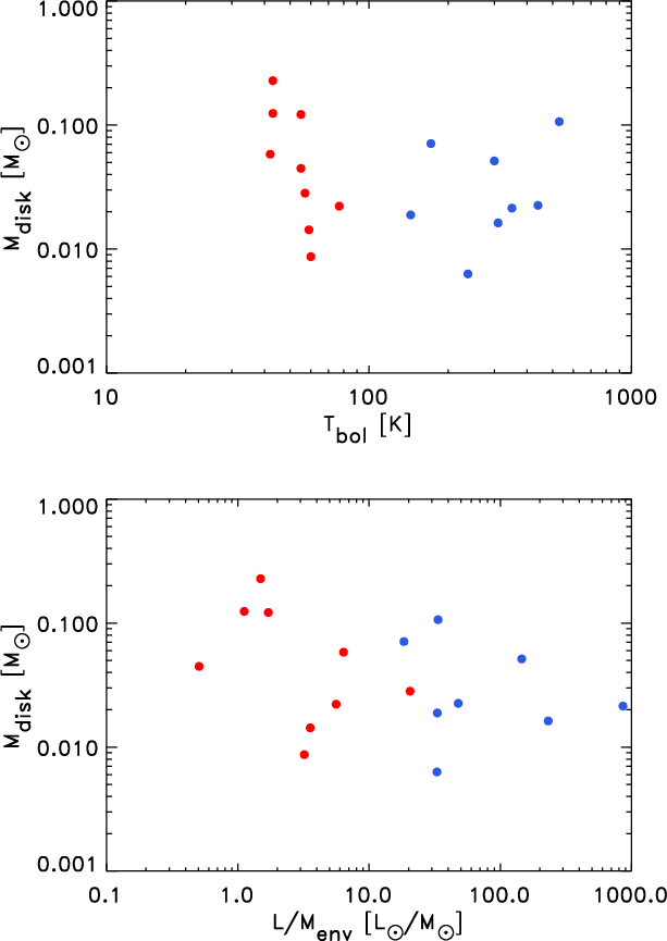
|
Figure 16: Disk masses as function of bolometric temperature ( upper) and source luminosity/envelope mass ratio ( lower). In comparison to Fig. 9, the Class 0 disk masses have been decreased by a factor 2 and the Class I disk masses increased by a similar amount - simulating the evolutionary effect in the relationship between flux and disk mass suggested by Fig. 15. |
| Open with DEXTER | |
Other dust opacity laws or temperatures have been used in literature:
Andrews & Williams (2007b) adopted an empirical scaling based on modeling of the
disk SEDs, corresponding to an equivalent dust temperature of 20 K and
a dust opacity-law following Beckwith et al. (1990) normalized to the dust
opacity at 1000 GHz of 0.1 cm2 g-1 (for a dust-to-gas ratio of 1:100). The lower temperature leads to higher disk masses for a given
1.1 mm flux by a factor of 2.3 whereas their adopted dust opacity-law
corresponds to lower disk masses by a factor 2.0 compared to
ours. Likewise, Terebey et al. (1993) adopted a dust temperature of 40 K
and adopted a dust opacity law with a mass opacity at 250 ![]() m of
0.1 cm2 g-1. If compared at a common wavelength of 850
m of
0.1 cm2 g-1. If compared at a common wavelength of 850 ![]() m,
these three choices of parameters result in disk masses that agree
within
m,
these three choices of parameters result in disk masses that agree
within ![]() 15% from the middle value from Andrews & Williams (2007b).
15% from the middle value from Andrews & Williams (2007b).
However, systematic changes in the dust properties occurring during
the evolution of the young protostars could have an important effect
on our derived disk masses and observed trends. For example, the dust
opacities at 500 ![]() m-1 mm from Ossenkopf & Henning (1994) increase by as
much as an order of magnitude depending on the density at which the
grains have coagulated, although the effect is significantly smaller
for grains with ice mantles. As shown by D'Alessio et al. (2001) grain
growth increases the dust opacity at a specific wavelength,
m-1 mm from Ossenkopf & Henning (1994) increase by as
much as an order of magnitude depending on the density at which the
grains have coagulated, although the effect is significantly smaller
for grains with ice mantles. As shown by D'Alessio et al. (2001) grain
growth increases the dust opacity at a specific wavelength, ![]() ,
as long as the largest grains are smaller than
,
as long as the largest grains are smaller than ![]() .
In a
scenario where grains grow toward sizes inferred for T Tauri disks
(
.
In a
scenario where grains grow toward sizes inferred for T Tauri disks
(![]() 1 mm; e.g., D'Alessio et al. 2001) as the protostellar system
evolve through its embedded stages the derived disk masses for the
more evolved sources would be overestimated under our assumptions of
an unchanging dust opacity law. This would work in the opposite
direction of the temperature effect - toward even more massive disks
in the Class 0 compared to Class I stages. It cannot be ruled out that
grain growth would appear in a fashion not straightforwardly
increasing with ``age'' of the studied young stellar objects, e.g., if
the observed dust in the Class 0 sources is located in regions with
relatively higher densities for a significant fraction of time. Based
on the current observational data, it is not possible to separate
these scenarios, however: further resolved multi-wavelength images of
the dust continuum emission from the envelopes and disks around
protostars or of well-calibrated gas tracers (taking their chemistry
into account) are required.
1 mm; e.g., D'Alessio et al. 2001) as the protostellar system
evolve through its embedded stages the derived disk masses for the
more evolved sources would be overestimated under our assumptions of
an unchanging dust opacity law. This would work in the opposite
direction of the temperature effect - toward even more massive disks
in the Class 0 compared to Class I stages. It cannot be ruled out that
grain growth would appear in a fashion not straightforwardly
increasing with ``age'' of the studied young stellar objects, e.g., if
the observed dust in the Class 0 sources is located in regions with
relatively higher densities for a significant fraction of time. Based
on the current observational data, it is not possible to separate
these scenarios, however: further resolved multi-wavelength images of
the dust continuum emission from the envelopes and disks around
protostars or of well-calibrated gas tracers (taking their chemistry
into account) are required.
6.2 Collapse and disk formation models
Power-law density profiles are simplified parameterizations of the underlying envelope density profile and the envelopes are not spherical due to, e.g., rotation and the action of protostellar outflows.
In the framework of the Shu (1977) and Terebey et al. (1984) models for
inside-out collapsing envelopes, the density profile flattens from a
stationary r-2 density profile through a free-falling r-1.5profile to a flattened inner envelope where the angular momentum
roughly balances gravity. Terebey et al. (1993) examined the millimeter
emission from such envelope models using analytical descriptions for
the envelope density and temperature profiles and used those to
compare IRAM 30 m single-dish continuum observations (11
![]() ;
at
1.3 mm) to OVRO interferometric observations (4-10
;
at
1.3 mm) to OVRO interferometric observations (4-10
![]() ;
at
2.7 mm). Consistent with Fig. 6 they found that the
emission in the interferometric observations is completely dominated
by a central compact component whereas most of the observed
single-dish flux in fact has its origin in the collapsing
envelope. The dominance of the disk to the interferometric flux was
found by Terebey et al. to be due to (i) the smaller
beam of the interferometric data and negligible envelope mass on those
scales and; (ii) the steeper wavelength dependence found for the
dust emission in the optically thin envelope.
;
at
2.7 mm). Consistent with Fig. 6 they found that the
emission in the interferometric observations is completely dominated
by a central compact component whereas most of the observed
single-dish flux in fact has its origin in the collapsing
envelope. The dominance of the disk to the interferometric flux was
found by Terebey et al. to be due to (i) the smaller
beam of the interferometric data and negligible envelope mass on those
scales and; (ii) the steeper wavelength dependence found for the
dust emission in the optically thin envelope.
We expand this analysis by introducing the formation of a circumstellar viscous disk in the center using the models of Visser et al. (2009) and following the evolution of the submillimeter brightness profiles observed by an interferometer: Visser et al. adopted the framework of Cassen & Moosman (1981) and Terebey et al. (1984) to describe a collapsing envelope and introduced the formation and growth of a 2-dimensional central disk and star similar to, e.g., Yorke & Bodenheimer (1999). The models of Visser et al. also include the presence of an outflow cavity with a growing opening angle through the evolution consistent with observations (e.g., Arce & Sargent 2006). Using the axisymmetric radiative transfer code ``RADMC'' (Dullemond & Dominik 2004), Visser et al. calculated the temperature profile for time-steps in the above model description and furthermore followed the chemical history of particles during the collapse and disk formation. For this purpose, we adopt the temperature and density profiles of the envelope (with outflow cavity) and disk from Visser et al., as well as their prescription for the evolution of the stellar luminosity and effective temperature and dust parameters, and ray-trace these. Figure 17 shows the evolution of the predicted visibility curves at different time-steps for two representative models from the grid of Visser et al.
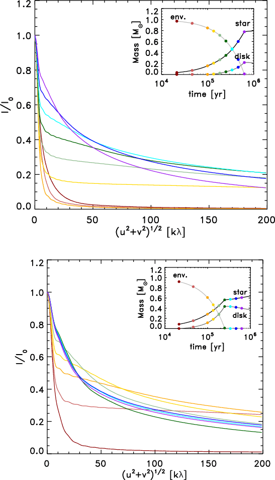
|
Figure 17:
Evolution of the predicted visibility amplitude curves (normalized by
the zero-spacing flux) as function of projected baseline lengths for two
models for envelope collapse and disk formation from Visser et al. (2009)
characterized by the solid-body rotation rate, |
| Open with DEXTER | |
Both panels clearly illustrate the effect discussed above: until the
formation of the circumstellar disk more than 95% of the total flux
at a given wavelength is emitted on baselines shorter than 50 k![]() - corresponding to a ratio between the 1.1 mm
interferometric flux and the peak 850
- corresponding to a ratio between the 1.1 mm
interferometric flux and the peak 850 ![]() m single-dish flux of less
than a few % (depending on the exact spectral slope between the
observations at these differing wavelengths) in accordance with the
results above. Once the disk is formed, the longer baseline flux
rapidly increases - first simultaneously on all baselines and then
more rapidly on the shorter baselines as the disk grows to sizes large
enough to be resolved by the interferometric observations. It should
be noted that even though the outflow cavity is opened up early in the
evolution of the collapsing protostar, it does not provide significant
compact emission, e.g., due to heated material in the outflow cavity
walls, to affect the evolution of the observed interferometric flux.
m single-dish flux of less
than a few % (depending on the exact spectral slope between the
observations at these differing wavelengths) in accordance with the
results above. Once the disk is formed, the longer baseline flux
rapidly increases - first simultaneously on all baselines and then
more rapidly on the shorter baselines as the disk grows to sizes large
enough to be resolved by the interferometric observations. It should
be noted that even though the outflow cavity is opened up early in the
evolution of the collapsing protostar, it does not provide significant
compact emission, e.g., due to heated material in the outflow cavity
walls, to affect the evolution of the observed interferometric flux.
An alternative explanation to the disk hypothesis favored in this work
is that there is an enhancement of the density in the envelope profile
at small scales. As an example, Chiang et al. (2008) adopted the
theoretical collapse models of Tassis & Mouschovias (2005) and compared those to
2.7 mm interferometric data from Looney et al. (2000). The models of
Tassis & Mouschovias (2005) simulate the formation of a protostellar object from a
cloud core in the presence of magnetic fields. In their simulation,
ambipolar diffusion leads to the formation of a thermally and
magnetically super-critical core which contracts
dynamically. Initially this core has a density profile
![]() ,
but as mass and magnetic flux is accreted from the envelope
onto the central protostar, a region of enhanced magnetic fields is
formed driving an outward-propagating shock and causing a density
enhancement growing quasi-periodically from scales of
,
but as mass and magnetic flux is accreted from the envelope
onto the central protostar, a region of enhanced magnetic fields is
formed driving an outward-propagating shock and causing a density
enhancement growing quasi-periodically from scales of
![]() 100 AU. This density enhancement on small scales will result in
a compact component observable by the interferometer which is slightly
resolved on long baselines and thereby in some cases alleviates the
need for a circumstellar disk on those scales as shown by
Chiang et al. (2008).
100 AU. This density enhancement on small scales will result in
a compact component observable by the interferometer which is slightly
resolved on long baselines and thereby in some cases alleviates the
need for a circumstellar disk on those scales as shown by
Chiang et al. (2008).
Still, the conclusions of both studies are similar: a density enhancement is required in the collapsing envelope on small scales - above what would be expected from, e.g., a free-falling envelope. The question is whether this component is inherent to the collapse profile or the first sign of the formation of a circumstellar disk. A straightforward, although currently observationally challenging, way to address this issue is through resolved line observations of the innermost envelope: the resolved line observations of the Class I sources in this sample (Lommen et al. 2008; Brinch et al. 2007) show clear signatures of Keplerian rotation, which argues in favor of the disk scenario for the sources in those evolutionary stages at least. For the more deeply embedded protostars future ALMA observations are needed to confirm the dynamical nature of the central compact dust component.
6.3 Constraints on evolutionary models
The presented observations and methodology make it possible to
directly constrain models for the evolution of young stellar objects -
in particular, concerning the transport of matter from the larger
scale envelope to the central star. This is in principle also the most
direct way for estimating the evolutionary status of individual young
stellar objects - rather than indirect indicators such as their
spectral energy distributions or similar. Figure 18
compares the predicted stellar and disk masses relative to the
envelope masses (i.e.,
![]() vs.
vs.
![]() )
from the models of Visser et al. (2009) to our
observed values. The thickened part of the lines in this plot
indicates where the Class 0 and I sources would fall on the
evolutionary track given their measured
)
from the models of Visser et al. (2009) to our
observed values. The thickened part of the lines in this plot
indicates where the Class 0 and I sources would fall on the
evolutionary track given their measured
![]() ratios.
ratios.
For the observed ratios of
![]() for the Class 0
sources, the models predict ratios of stellar to envelope masses
for the Class 0
sources, the models predict ratios of stellar to envelope masses
![]() in the range
in the range ![]() 0.2-0.6, i.e.,
systems that have accreted
0.2-0.6, i.e.,
systems that have accreted ![]() 15-40% of their final mass -
in accordance with the phenomenological definition of objects in the
Class 0 stage. Likewise the Class I sources are predicted to have more
massive stars than envelopes - again, in accordance with the
phenomenological distinction between Class 0 and I objects. For the
Class I sources with measured stellar masses, the observed
disk-to-stellar mass ratios are in the 1-10% range, whereas the
models predict a higher ratio of 20-25% in the late Class I stage
(i.e., overestimate the disk mass relative to the stellar mass). It
is seen that the predicted stellar masses for the Class 0 sources with
this model are a
15-40% of their final mass -
in accordance with the phenomenological definition of objects in the
Class 0 stage. Likewise the Class I sources are predicted to have more
massive stars than envelopes - again, in accordance with the
phenomenological distinction between Class 0 and I objects. For the
Class I sources with measured stellar masses, the observed
disk-to-stellar mass ratios are in the 1-10% range, whereas the
models predict a higher ratio of 20-25% in the late Class I stage
(i.e., overestimate the disk mass relative to the stellar mass). It
is seen that the predicted stellar masses for the Class 0 sources with
this model are a
![]() .
.
The low disk masses relative to stellar masses suggest that material is quickly and efficiently accreted from the envelope through the disk onto the star. This is also directly illustrated by the comparison between the observed and modeled stellar-to-disk mass ratios for the five Class I sources for which both have been determined. For the Class I sources the observed disk masses are 1-10% of the corresponding stellar masses whereas the models predict ratios of 20-25%. This suggests that the material is processed more quickly through the circumstellar disks than what is given by the models. Looney et al. (2003) suggested that this was the case based on their conclusion that Class 0 protostars have disks that are not more massive than their Class I counterparts. Our results are in agreement with this general conclusion.
It is worth emphasizing though, that our analysis does find evidence for disks around the Class 0 sources. If the Class 0 sources indeed are precursors to the Class I sources in this sample, this in turn would suggest that circumstellar disks are formed early in the evolution of low-mass protostars. Without resolved line observations it is not possible to address whether these disks in fact are rotationally supported Keplerian disks. The absence of a clear rotation signature in the disk around NGC 1333-IRAS2A (Brinch et al. 2009) combined with its large apparent size from the dust continuum measurements (Jørgensen et al. 2005a) could perhaps be consistent with it being an unstable ``pseudo-disk'' as in the framework of Galli & Shu (1993b,a) - although it may also simply be that the evolutionary time-scale for IRAS2A still has been too short for the disk to establish Keplerian rotation (Brinch et al. 2009).
An open question in the comparison to the theoretical models is how important outflows are in carrying away envelope material. The observed increasing opening angles of outflows with increasing age of the protostar has been interpreted as evidence for the erosion of the protostellar envelope by the outflow (Arce & Sargent 2006; Velusamy & Langer 1998) in part explaining the observed shift in the peak between the core and initial mass function (e.g., Myers 2008). In the models of Visser et al. (2009) and shown in Fig. 18 the amount of material carried away by the outflow only amounts to a few percent. Generally, a more efficient outflow dispersal of the core would decrease the disk and stellar masses relative to the envelope masses - corresponding to a diagonal shift of a given modeled object in Fig. 18 - roughly along the evolutionary tracks. Therefore, unless the outflow preferentially alter the accretion onto the disk relative to the star, the ratio between the masses of the two will not be changed and thus also not the implications discussed here.
A final interesting possibility is that the flat distribution of disk
masses from the Class 0 to I stages reflects the stability of the
disks, given the suggestion that the luminosity problem of low-mass
protostars can be explained if mass is accreted on large scales in the
disks and from there onto the central star in highly episodic events:
in their models for collapse of a dense core and formation of a
protostar and disk, Vorobyov & Basu (2006) find strong episodic accretion
once the disk has formed which keeps its mass lower than the stellar
mass at all points during the protostellar evolution. Given that the
recent Spitzer/c2d results suggest that the luminosity problem extends
to the earliest Class 0 stages (Evans et al. 2009), it is tempting to
suggest that material already at these stages indeed ends up in
circumstellar disks and from there is accreted toward the central star
in bursts when a local instability criterion is exceeded - e.g.,
related to comparison between the disk size/mass and stellar
mass. This could in turn flatten the distribution of disk masses as
function of bolometric temperatures, with an upper envelope of disk
masses of 0.05-0.1 ![]() corresponding to the maximum values
observed for our sample of Class 0 and I protostars. It should be
emphasized that since our sample is rather small, biases may have been
introduced in its selection. Future studies of larger samples of
protostars with current and upcoming (sub)millimeter interferometers
will be needed to address this potential bias.
corresponding to the maximum values
observed for our sample of Class 0 and I protostars. It should be
emphasized that since our sample is rather small, biases may have been
introduced in its selection. Future studies of larger samples of
protostars with current and upcoming (sub)millimeter interferometers
will be needed to address this potential bias.
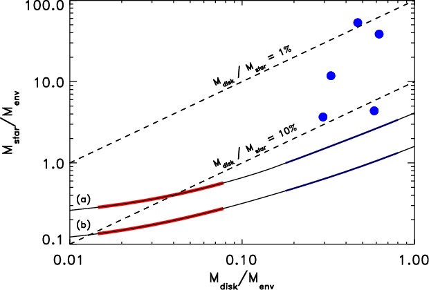
|
Figure 18:
Predicted stellar mass,
|
| Open with DEXTER | |
7 Summary and outlook
We have presented a comprehensive analysis of the dust continuum envelope emission of a sample of 20 embedded low-mass YSOs (Class 0 and I) based on submillimeter interferometric observations from the Submillimeter Array probing scales of a few hundred AU and single-dish continuum observations from the JCMT (scales larger than 2000 AU). In addition we discuss HCO+ 3-2 line emission for the Class I sources in the sample. With these data we have characterized the evolution of the three main components YSOs - the envelope, disk and stellar masses - and the relation between these compared to theoretical models. The main conclusions are as follows:- 1.
- The millimeter dust continuum emission from both the interferometric observations (on scales of 250-500 AU) and single-dish observations (scales larger than 2000 AU) decreases in strength from the more deeply embedded Class 0 to the more evolved Class I sources. Relative to the single-dish data, the interferometric continuum flux at millimeter wavelengths increases toward the more evolved sources.
- 2.
- Through comparison to predictions from dust radiative transfer models, an upper limit on the contribution from protostellar envelope to the interferometric continuum flux is estimated - relative to the continuum flux measured on larger scales with single-dish telescopes. For the Class I sources about 87% of the observed SMA continuum flux (median value for the sample of Class I sources) has its origin in the circumstellar disks with the remainder coming from the large-scale envelope. For the Class 0 sources, 68% of the interferometric emission is related to the circumstellar disks.
- 3.
- Using empirical relationships between the envelope and disk fluxes and their masses from the radiative transfer models, the observations show that the disk-to-envelope mass ratio increases from about 1-10% in the Class 0 stage to about 20-60% in the Class I stage, reflecting the dissipation of the envelope in the more evolved stages.
- 4.
- The compact interferometric fluxes due to disks are
observed to decrease from the Class 0 to the Class I
objects. However, this decrease is largely due to the changing
physical properties, in particular disk temperature, during this
phase. If these effects are taken into account, the disk mass
shows no significant trends from the Class 0 to I stages and is
typically 0.05
 ,
albeit with significant scatter. Thus,
no evidence is seen for significant disk mass growth from the
Class 0 to the Class I stages.
,
albeit with significant scatter. Thus,
no evidence is seen for significant disk mass growth from the
Class 0 to the Class I stages.
- 5.
- Four Class I sources in the sample show evidence of Keplerian
rotation in HCO+ 3-2, and for IRS 43 also in HCN 3-2. IRS 63
and IRS 43 show evidence for elongated ``continuum disks'' at
1.1 mm. For IRS 43 both the ``continuum disk'' and the HCO+ 3-2
emission coincides with a dark lane in the HST 1.6
 m images -
and orientated perpendicular to the direction of the protostellar
outflow. For the four Class I sources we derive central masses of
0.3-2.5
from the Keplerian rotation curve.
m images -
and orientated perpendicular to the direction of the protostellar
outflow. For the four Class I sources we derive central masses of
0.3-2.5
from the Keplerian rotation curve.
- 6.
- The high excitation HCO+ and HCN lines appear to be good tracers of the motions in the inner envelopes and disks, although in the most massive envelopes their use for this purpose is limited by the lines of the main isotopes being optical thick. Future observations with ALMA will allow similar studies using the less abundant isotopologues.
- 7.
- We compare the derived envelope and stellar masses to models for the mass evolution in a collapsing protostellar system including the formation and growth of a central circumstellar disk (Visser et al. 2009). The data are in agreement with phenomenological definition of Class 0 sources having accreted less, and Class I sources more, than half of their final mass. The models cannot explain the observed stellar masses for the handful of Class I sources for which these have been measured from the disk dynamical structure: generally the models produce too massive disks relative to their stellar masses.
- 8.
- Taken together these results suggest that circumstellar disks are established early in the evolution of low-mass protostars, but at the same time transport material rapidly from the larger scale envelopes onto the central stars. This may occur in episodic events, which may explain why the ``luminosity problem'' (that embedded YSOs are under-luminous compared to the theoretical predictions from pure accretion models) appears already during the Class 0 protostellar stages (e.g., Evans et al. 2009).
Future ALMA observations will provide the sensitivity to molecules that are less abundant, and thus not severely optically thick in the outer envelopes, and thus a tracer of this structure. With ALMA it will also be possible to perform larger surveys of a statistically more unbiased sample of YSOs to constrain the evolution more directly. This will for example address whether traditional classification schemes for young stellar objects need to be recalibrated, whether the episodic accretion scenarios for YSOs are tied to the properties of their circumstellar disk, whether there are significant variations between accretion histories of protostars in different star forming environments, and what fraction of the envelope material is accreted onto the star and what fraction is carried away by the outflows.
AcknowledgementsWe thank the referee for good suggestions about the presentation of these results. It is also a pleasure to thank the Submillimeter Array staff for help in carrying out observations and technical assistance with the resulting data. The Submillimeter Array is a joint project between the Smithsonian Astrophysical Observatory and the Academia Sinica Institute of Astronomy and Astrophysics, and is funded by the Smithsonian Institution and the Academia Sinica. This research was based in part on observations from the James Maxwell Telescope archive at the Canadian Astronomy Data Centre operated by the National Research Council of Canada with the support of the Canadian Space Agency. It is also used observations made with the NASA/ESA Hubble Space Telescope, obtained from the data archive at the Space Telescope Institute. STScI is operated by the association of Universities for Research in Astronomy, Inc. under the NASA contract NAS 5-26555. Astrochemistry in Leiden is supported by a Spinoza Grant from the Netherlands Organization for Scientific Research (NWO) and a NOVA grant. The research of T.L.B. was supported by NASA Origins grant NNX09AB89G.
References
- Allen, L. E., Myers, P. C., Di Francesco, J., et al. 2002, ApJ, 566, 993 [CrossRef] [NASA ADS]
- André, P., & Montmerle, T. 1994, ApJ, 420, 837 [CrossRef] [NASA ADS]
- André, P., Ward-Thompson, D., & Barsony, M. 1993, ApJ, 406, 122 [CrossRef] [NASA ADS]
- André, P., Ward-Thompson, D., & Barsony, M. 2000, in Protostars and Planets IV, ed. V. Mannings, A. P. Boss, & S. S. Russell (Tucson: University of Arizona Press), 59
- Andrews, S. M., & Williams, J. P. 2005, ApJ, 631, 1134 [CrossRef] [NASA ADS]
- Andrews, S. M., & Williams, J. P. 2007a, ApJ, 671, 1800 [CrossRef] [NASA ADS]
- Andrews, S. M., & Williams, J. P. 2007b, ApJ, 659, 705 [CrossRef] [NASA ADS] (In the text)
- Arce, H. G., & Sargent, A. I. 2006, ApJ, 646, 1070 [CrossRef] [NASA ADS] (In the text)
- Barsony, M., Kenyon, S. J., Lada, E. A., & Teuben, P. J. 1997, ApJS, 112, 109 [CrossRef] [NASA ADS]
- Basu, S. 1998, ApJ, 509, 229 [CrossRef] [NASA ADS]
- Beckwith, S. V. W., Sargent, A. I., Chini, R. S., & Guesten, R. 1990, AJ, 99, 924 [CrossRef] [NASA ADS]
- Brinch, C., Crapsi, A., Jørgensen, J. K., Hogerheijde, M. R., & Hill, T. 2007, A&A, 475, 915 [EDP Sciences] [CrossRef] [NASA ADS] (In the text)
- Brinch, C., Jørgensen, J. K., & Hogerheijde, M. R. 2009, A&A, 502, 199 [EDP Sciences] [CrossRef] [NASA ADS]
- Brown, D. W., & Chandler, C. J. 1999, MNRAS, 303, 855 [CrossRef] [NASA ADS]
- Cassen, P., & Moosman, A. 1981, Icarus, 48, 353 [CrossRef] [NASA ADS]
- Chandler, C. J., Terebey, S., Barsony, M., Moore, T. J. T., & Gautier, T. N. 1996, ApJ, 471, 308 [CrossRef] [NASA ADS] (In the text)
- Chiang, H.-F., Looney, L. W., Tassis, K., Mundy, L. G., & Mouschovias, T. C. 2008, ApJ, 680, 474 [CrossRef] [NASA ADS] (In the text)
- Curiel, S., Girart, J. M., Rodríguez, L. F., & Cantó, J. 2003, ApJ, 582, L109 [CrossRef] [NASA ADS] (In the text)
- D'Alessio, P., Calvet, N., & Hartmann, L. 2001, ApJ, 553, 321 [CrossRef] [NASA ADS] (In the text)
- Di Francesco, J., Johnstone, D., Kirk, H., MacKenzie, T., & Ledwosinska, E. 2008, ApJS, 175, 277 [CrossRef] [NASA ADS]
- Duchêne, G., Bouvier, J., Bontemps, S., André, P., & Motte, F. 2004, A&A, 427, 651 [EDP Sciences] [CrossRef] [NASA ADS] (In the text)
- Dullemond, C. P., & Dominik, C. 2004, A&A, 417, 159 [EDP Sciences] [CrossRef] [NASA ADS] (In the text)
- Dunham, M. M., Crapsi, A., Evans, II, N. J., et al. 2008, ApJS, 179, 249 [CrossRef] [NASA ADS]
- Eisner, J. A., Hillenbrand, L. A., Carpenter, J. M., & Wolf, S. 2005, ApJ, 635, 396 [CrossRef] [NASA ADS]
- Enoch, M. L., Glenn, J., Evans, II, N. J., et al. 2007, ApJ, 666, 982 [CrossRef] [NASA ADS] (In the text)
- Evans, N. J. 1999, ARA&A, 37, 311 [CrossRef] [NASA ADS] (In the text)
- Evans, N. J., Dunham, M. M., Jørgensen, J. K., et al. 2009, ApJS, 181, 321 [CrossRef] [NASA ADS]
- Galli, D., & Shu, F. H. 1993a, ApJ, 417, 220 [CrossRef] [NASA ADS]
- Galli, D., & Shu, F. H. 1993b, ApJ, 417, 243 [CrossRef] [NASA ADS] (In the text)
- Girart, J. M., Rodríguez, L. F., & Curiel, S. 2000, ApJ, 544, L153 [CrossRef] [NASA ADS]
- Girart, J. M., Curiel, S., Rodríguez, L. F., et al. 2004, AJ, 127, 2969 [CrossRef] [NASA ADS] (In the text)
- Girart, J. M., Rao, R., & Estalella, R. 2009, ApJ, 694, 56 [CrossRef] [NASA ADS] (In the text)
- Grosso, N., Alves, J., Neuhäuser, R., & Montmerle, T. 2001, A&A, 380, L1 [EDP Sciences] [CrossRef] [NASA ADS] (In the text)
- Gutermuth, R. A., Myers, P. C., Megeath, S. T., et al. 2008, ApJ, 674, 336 [CrossRef] [NASA ADS]
- Haisch, Jr., K. E., Greene, T. P., Barsony, M., & Stahler, S. W. 2004, AJ, 127, 1747 [CrossRef] [NASA ADS]
- Hatchell, J., & Fuller, G. A. 2008, A&A, 482, 855 [EDP Sciences] [CrossRef] [NASA ADS] (In the text)
- Hatchell, J., Fuller, G. A., Richer, J. S., Harries, T. J., & Ladd, E. F. 2007, A&A, 468, 1009 [EDP Sciences] [CrossRef] [NASA ADS] (In the text)
- Ho, P. T. P., Moran, J. M., & Lo, K. Y. 2004, ApJ, 616, L1 [CrossRef] [NASA ADS]
- Hogerheijde, M. R., & Sandell, G. 2000, ApJ, 534, 880 [CrossRef] [NASA ADS]
- Hogerheijde, M. R., van Dishoeck, E. F., Blake, G. A., & van Langevelde, H. J. 1997a, ApJ, 489, 293 [CrossRef] [NASA ADS]
- Hogerheijde, M. R., van Langevelde, H. J., Mundy, L. G., Blake, G. A., & van Dishoeck, E. F. 1997b, ApJ, 490, L99 [CrossRef] [NASA ADS]
- Hogerheijde, M. R., van Dishoeck, E. F., Blake, G. A., & van Langevelde, H. J. 1998, ApJ, 502, 315 [CrossRef] [NASA ADS] (In the text)
- Ivezic, Z., Nenkova, M., & Elitzur, M. 1999, User Manual for DUSTY, University of Kentucky Internal Report
- Jørgensen, J. K. 2004, A&A, 424, 589 [EDP Sciences] [CrossRef] [NASA ADS] (In the text)
- Jørgensen, J. K., Schöier, F. L., & van Dishoeck, E. F. 2002, A&A, 389, 908 [EDP Sciences] [CrossRef] [NASA ADS]
- Jørgensen, J. K., Hogerheijde, M. R., van Dishoeck, E. F., Blake, G. A., & Schöier, F. L. 2004a, A&A, 413, 993 [EDP Sciences] [CrossRef] [NASA ADS] (In the text)
- Jørgensen, J. K., Schöier, F. L., & van Dishoeck, E. F. 2004b, A&A, 416, 603 [EDP Sciences] [CrossRef] [NASA ADS]
- Jørgensen, J. K., Bourke, T. L., Myers, P. C., et al. 2005a, ApJ, 632, 973 [CrossRef] [NASA ADS]
- Jørgensen, J. K., Lahuis, F., Schöier, F. L., et al. 2005b, ApJ, 631, L77 [CrossRef] [NASA ADS]
- Jørgensen, J. K., Harvey, P. M., Evans, N. J. I., et al. 2006, ApJ, 645, 1246 [CrossRef] [NASA ADS] (In the text)
- Jørgensen, J. K., Bourke, T. L., Myers, P. C., et al. 2007a, ApJ, 659, 479 [CrossRef] [NASA ADS]
- Jørgensen, J. K., Johnstone, D., Kirk, H., & Myers, P. C. 2007b, ApJ, 656, 293 [CrossRef] [NASA ADS] (In the text)
- Jørgensen, J. K., Johnstone, D., Kirk, H., et al. 2008, ApJ, 683, 822 [CrossRef] [NASA ADS] (In the text)
- Keene, J., & Masson, C. R. 1990, ApJ, 355, 635 [CrossRef] [NASA ADS] (In the text)
- Kenyon, S. J., Hartmann, L. W., Strom, K. M., & Strom, S. E. 1990, AJ, 99, 869 [CrossRef] [NASA ADS]
- Lay, O. P., Carlstrom, J. E., Hills, R. E., & Phillips, T. G. 1994, ApJ, 434, L75 [CrossRef] [NASA ADS] (In the text)
- Leous, J. A., Feigelson, E. D., André, P., & Montmerle, T. 1991, ApJ, 379, 683 [CrossRef] [NASA ADS]
- Lommen, D., Jørgensen, J. K., van Dishoeck, E. F., & Crapsi, A. 2008, A&A, 481, 141 [EDP Sciences] [CrossRef] [NASA ADS]
- Looney, L. W., Mundy, L. G., & Welch, W. J. 2000, ApJ, 529, 477 [CrossRef] [NASA ADS]
- Looney, L. W., Mundy, L. G., & Welch, W. J. 2003, ApJ, 592, 255 [CrossRef] [NASA ADS] (In the text)
- Looney, L. W., Tobin, J. J., & Kwon, W. 2007, ApJ, 670, L131 [CrossRef] [NASA ADS] (In the text)
- Montmerle, T., Grosso, N., Tsuboi, Y., & Koyama, K. 2000, ApJ, 532, 1097 [CrossRef] [NASA ADS]
- Mundy, L. G., Looney, L. W., Erickson, W., et al. 1996, ApJ, 464, L169 [CrossRef] [NASA ADS] (In the text)
- Myers, P. C., & Ladd, E. F. 1993, ApJ, 413, L47 [CrossRef] [NASA ADS] (In the text)
- Myers, P. C. 2008, ApJ, 687, 340 [CrossRef] [NASA ADS] (In the text)
- Ossenkopf, V., & Henning, T. 1994, A&A, 291, 943 [NASA ADS] (In the text)
- Padgett, D. L., Rebull, L. M., Stapelfeldt, K. R., et al. 2008, ApJ, 672, 1013 [CrossRef] [NASA ADS] (In the text)
- Qi, C. 2008, The MIR Cookbook, The Submillimeter Array / Harvard-Smithsonian Center for Astrophysics(http://cfa-www.harvard.edu/ cqi/mircook.html) (In the text)
- Sault, R. J., Teuben, P. J., & Wright, M. C. H. 1995, in Astronomical Data Analysis Software and Systems IV, ed. R. A. Shaw, H. E. Payne, & J. J. E. Hayes, PASP Conf. Ser., 77, 433
- Schöier, F. L., Jørgensen, J. K., van Dishoeck, E. F., & Blake, G. A. 2002, A&A, 390, 1001 [EDP Sciences] [CrossRef] [NASA ADS]
- Schöier, F. L., Jørgensen, J. K., van Dishoeck, E. F., & Blake, G. A. 2004, A&A, 418, 185 [EDP Sciences] [CrossRef] [NASA ADS]
- Shirley, Y. L., Evans, N. J., & Rawlings, J. M. C. 2002, ApJ, 575, 337 [CrossRef] [NASA ADS] (In the text)
- Shu, F. H. 1977, ApJ, 214, 488 [CrossRef] [NASA ADS] (In the text)
- Stutz, A. M., Rubin, M., Werner, M. W., et al. 2008, ApJ, 687, 389 [CrossRef] [NASA ADS] (In the text)
- Tassis, K., & Mouschovias, T. C. 2005, ApJ, 618, 783 [CrossRef] [NASA ADS]
- Terebey, S., Shu, F. H., & Cassen, P. 1984, ApJ, 286, 529 [CrossRef] [NASA ADS] (In the text)
- Terebey, S., Chandler, C. J., & Andre, P. 1993, ApJ, 414, 759 [CrossRef] [NASA ADS] (In the text)
- Terebey, S., van Buren, D., Padgett, D. L., Hancock, T., & Brundage, M. 1998, ApJ, 507, L71 [CrossRef] [NASA ADS]
- Terebey, S., Van Buren, D., Matthews, K., & Padgett, D. L. 2000, AJ, 119, 2341 [CrossRef] [NASA ADS] (In the text)
- Tobin, J. J., Hartmann, L., Calvet, N., & D'Alessio, P. 2008, ApJ, 679, 1364 [CrossRef] [NASA ADS] (In the text)
- Tsuboi, Y., Imanishi, K., Koyama, K., Grosso, N., & Montmerle, T. 2000, ApJ, 532, 1089 [CrossRef] [NASA ADS]
- Ulrich, R. K. 1976, ApJ, 210, 377 [CrossRef] [NASA ADS] (In the text)
- van der Tak, F. F. S., Black, J. H., Schöier, F. L., Jansen, D. J., & van Dishoeck, E. F. 2007, A&A, 468, 627 [EDP Sciences] [CrossRef] [NASA ADS] (In the text)
- van Kempen, T. A., van Dishoeck, E. F., Salter, D. M., et al. 2009, A&A, 498, 167 [EDP Sciences] [CrossRef] [NASA ADS]
- Velusamy, T., & Langer, W. D. 1998, Nature, 392, 685 [CrossRef] [NASA ADS] (In the text)
- Visser, R., van Dishoeck, E. F., Doty, S. D., & Dullemond, C. P. 2009, A&A, 495, 881 [EDP Sciences] [CrossRef] [NASA ADS] (In the text)
- Vorobyov, E. I., & Basu, S. 2006, ApJ, 650, 956 [CrossRef] [NASA ADS] (In the text)
- Ward-Thompson, D. 2007, Joint 32nd International Conference on Infrared and Millimeter Waves,and 15th International Conference on Terahertz Electronics. IRMMW-THz, ed. M. Griffin, P. C. Hargrave, T. J. Parker, & K. P. Wood, 720 (In the text)
- Weintraub, D. A., Kastner, J. H., Griffith, L. L., & Campins, H. 1993, AJ, 105, 271 [CrossRef] [NASA ADS] (In the text)
- Yorke, H. W., & Bodenheimer, P. 1999, ApJ, 525, 330 [CrossRef] [NASA ADS] (In the text)
- Young, E. T., Lada, C. J., & Wilking, B. A. 1986, ApJ, 304, L45 [CrossRef] [NASA ADS]
- Young, C. H., Shirley, Y. L., Evans, N. J., & Rawlings, J. M. C. 2003, ApJS, 145, 111 [CrossRef] [NASA ADS] (In the text)
- Young, K. E., Enoch, M. L., Evans, II, N. J., et al. 2006, ApJ, 644, 326 [CrossRef] [NASA ADS] (In the text)
- Zhang, Q., Wootten, A., & Ho, P. T. P. 1997, ApJ, 475, 713 [CrossRef] [NASA ADS]
Online Material
Appendix A: The use of HCO+ as a dense gas tracer
A.1 Outflow cavities in TMR1, TMC1A and GSS30-IRS1
The HCO+ 3-2 alignment with the near-infrared scattering nebulosities in the HST images for TMR1, TMC1A and GSS30-IRS1 (Fig. 10) is similar to what has been found in high angular resolution observations of the lower excitation 1-0 transition in both Class I (Hogerheijde et al. 1997a) and Class 0 (Jørgensen 2004) sources.
The patterns in the velocity maps (Fig. 11) support the interpretation that the HCO+ 3-2 emission has its origin in one-side of the outflow cone: in all maps the HCO+ emission is blue-shifted with respect to the systemic velocity with the most extreme velocities (most blue-shifted) narrowly confined around the continuum position and material closer to the systemic velocity extending around this. This signature can best be understood in a simple geometry where HCO+ probes material in a large infalling protostellar envelope being swept up by the outflow, as illustrated in Fig. A.1. If the velocities in the swept-up material are relatively small (comparable to the infalling velocities in the envelope) and HCO+ 3-2 optically thick, the front-side of the envelope (toward us) will be slightly red-shifted due to the infall and thus obscure the outflowing material in the red-shifted cone on the far-side of the envelope (Fig. A.1), which in turn is resolved-out. In contrast, the outflow cone pointed toward us will be unobscured by the envelope. Likewise, the near-infrared scattered light from the red-lobe would largely be blocked - in contrast to the scattered emission from the outflow cavity on the front-side. An alternative explanation is that all the sources are at the far-side of their respective clouds, the red-shifted part of the outflow cone breaking out into a low-density medium not observable in the line tracers. This would require a rather sharp density gradient, however.
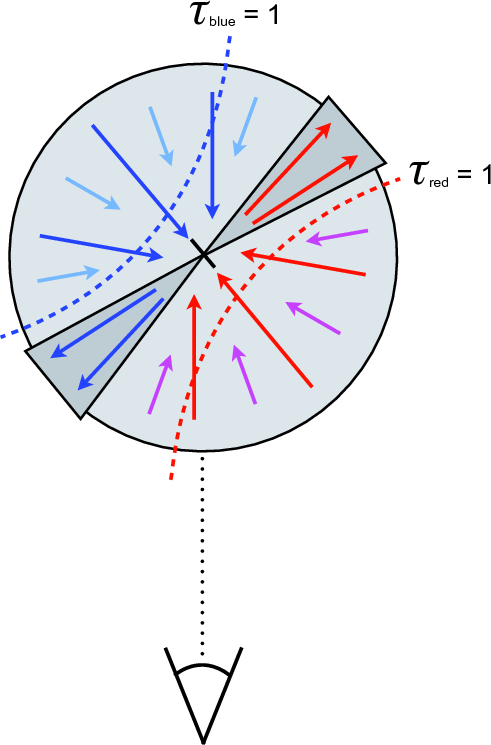
|
Figure A.1:
Schematic figure of a collapsing envelope with an outflow
sweeping up material. The dashed lines indicate the |
| Open with DEXTER | |
A.2 Limitations of HCO+ 3-2 as a tracer of disks
The results above suggest that HCO+ 3-2 is a good tracer of
motions in disks for envelopes that have already been largely
dispersed. For the more embedded YSOs, HCO+ 3-2 emission may be of
limited use as a tracer of rotation in the disk due to its optical
thickness. A simple estimate can be made of the typical envelope mass
below which HCO+ 3-2 line emission is optically thin in the
envelope and can be used as a tracer of the kinematics in the
innermost regions of the protostar. First, for typical envelope
parameters we expect temperatures in the range of 15-40 K and
densities of 104-107 cm-3. Using the Radex escape
probability code (van der Tak et al. 2007)![]() for these
parameters, the HCO+ 3-2 line has an optical thickness
for these
parameters, the HCO+ 3-2 line has an optical thickness
![]() 1
for an HCO+ column density of
1
for an HCO+ column density of
![]() cm-2 and a
line width of 1 km s-1. Secondly, we can estimate what density,
cm-2 and a
line width of 1 km s-1. Secondly, we can estimate what density,
![]() is required to reach that optical thickness in a
free-falling envelope with a power-law density profile,
is required to reach that optical thickness in a
free-falling envelope with a power-law density profile,
![]() at a size scale of 100 AU corresponding to the
region where the disk potentially forms, i.e., by simply estimating
at a size scale of 100 AU corresponding to the
region where the disk potentially forms, i.e., by simply estimating
![]() from
from
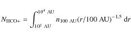
|
(A.1) |
with
Appendix B: Summary of observed Class I sources
B.1 IRS 43
IRS 43 (YLW15; Young et al. 1986) has been the target of numerous
studies across the full wavelength range. At radio wavelengths, IRS 43
is resolved into two separate components, YLW15-VLA1 and -VLA2 with a
separation of 0.6
![]() (Girart et al. 2000). From multi-epoch high
angular resolution radio data, these binary components were found to
show relative proper motions indicative of orbital motions in a
1.7
(Girart et al. 2000). From multi-epoch high
angular resolution radio data, these binary components were found to
show relative proper motions indicative of orbital motions in a
1.7 ![]() total mass binary
(Curiel et al. 2003). Girart et al. found that one of the two
components, VLA1, were resolved in observations at 3.6 and 6 cm with
the VLA with a deconvolved size of about 0.4
total mass binary
(Curiel et al. 2003). Girart et al. found that one of the two
components, VLA1, were resolved in observations at 3.6 and 6 cm with
the VLA with a deconvolved size of about 0.4
![]() along its major
axis and suggested that it was associated with a thermal radio jet. In
addition, IRS 43 is a peculiar X-ray emitter showing quasi-periodic
X-ray flares (Tsuboi et al. 2000) consistent with magnetic shearing and
reconnection between the central star and an accretion disk, with the
period suggesting a mass of the central star in the range
1.8-2.2
along its major
axis and suggested that it was associated with a thermal radio jet. In
addition, IRS 43 is a peculiar X-ray emitter showing quasi-periodic
X-ray flares (Tsuboi et al. 2000) consistent with magnetic shearing and
reconnection between the central star and an accretion disk, with the
period suggesting a mass of the central star in the range
1.8-2.2 ![]() (Montmerle et al. 2000).
(Montmerle et al. 2000).
The region was imaged in the near-infrared by Grosso et al. (2001) who discovered a set of ``embedded'' Herbig-Haro objects, well aligned with the thermal jet candidate from the centimeter observations of Girart et al. (2000). Spitzer Space Telescope images of the embedded Herbig-Haro objects (Fig. B.1) show the knots clearly along a line pointing directly back toward the group of objects where IRS 43 and another embedded protostar, IRS 44, is located. As also pointed out by Grosso et al., the association of the Herbig-Haro knots to IRS 43 is not unique: the nearby protostar, IRS 54 (see also Sect. B.5), also drives a large-scale, precessing outflow clearly seen in the Spitzer images in Fig. B.1.
The dotted lines in Fig. B.1 show the propagation of
the IRS 54 outflow, following the H2 emission in the eastern lobe
and assuming that the precession of the IRS 54 outflow is symmetric
around the protostar - thereby giving the expected location of the
western lobe. The western lobe in this case passes through the
location of the southern part of the near-infrared Herbig-Haro
objects: based on their morphologies in the higher resolution
near-infrared images, Grosso et al. (2001) suggested that these knots
(crosses in the lower left panel of Fig. B.1) are
indeed caused by the IRS 54 outflow with the northern knots (plus
signs in the lower left panel of Fig. B.1 related to
the IRS 43 outflow - the lower spatial resolution Spitzer images do
not reveal this distinction clearly, though. Some support for the
interpretation of Grosso et al. can be taken from the
morphology of another bow-shock seen in the Spitzer images at
![]() to the west of the near-infrared Herbig-Haro
knots. Together with the near-infrared Herbig Haro knots detected by
Grosso et al., this bow-shock is on the southern side of the
dashed-line suggesting that the dashed line indeed is delineating the
northern edge of the western lobe (and the southern edge of the
eastern lobe) of the IRS 54 outflow. It is also possible that another
source in the group encompassing IRS 43 could be responsible for the
Herbig-Haro knots: the main argument for the association to IRS 43 is
the coincidence with the radio jet and the identification of a
bow-shock south of IRS 43 in the near-infrared, possibly representing
the counter-jet (Grosso et al. 2001; Girart et al. 2000,2004).
to the west of the near-infrared Herbig-Haro
knots. Together with the near-infrared Herbig Haro knots detected by
Grosso et al., this bow-shock is on the southern side of the
dashed-line suggesting that the dashed line indeed is delineating the
northern edge of the western lobe (and the southern edge of the
eastern lobe) of the IRS 54 outflow. It is also possible that another
source in the group encompassing IRS 43 could be responsible for the
Herbig-Haro knots: the main argument for the association to IRS 43 is
the coincidence with the radio jet and the identification of a
bow-shock south of IRS 43 in the near-infrared, possibly representing
the counter-jet (Grosso et al. 2001; Girart et al. 2000,2004).
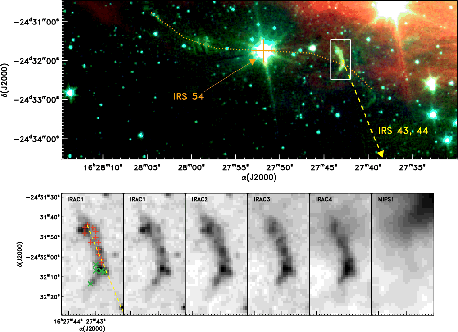
|
Figure B.1:
Upper panel: the region of the IRS 54 outflow as well
as the near-infrared Herbig-Haro objects from Spitzer observations
with 3.6 |
| Open with DEXTER | |
We detect IRS 43 in both HCO+ 3-2, HCN 3-2 and continuum. The HCN and HCO+ 3-2 emission is elongated in the W/NW-E/SE direction with a clear velocity gradient along its major axis. The major axis of the HCO+ and HCN 3-2 emission is close to the axis of the continuum emission - and perpendicular to the direction toward the Herbig-Haro objects (Fig. B.1; Grosso et al. 2001) and the thermal continuum jet (Girart et al. 2000).
B.2 TMR1 and TMC1A
Images of TMR1 using the HST/NICMOS at 1.6-2.1Both TMR1 and TMC1A are detected in continuum, together with HCO+and HCN 3-2. Both show clear evidence of the line emission being offset from the continuum peaks toward the outflow nebulosity observed in the near-infrared HST/NICMOS images - similar to the case for GSS30-IRS1. The offsets in the HCO+ 3-2 emission toward the two sources are similar to those observed in HCO+ 1-0 by Hogerheijde et al. (1998).
B.3 GSS30
The GSS30 region is the most complex of the studied fields associated with a clear near-infrared nebulosity. At least three young stellar objects (GSS30-IRS1, -IRS2 and -IRS3) are seen at infrared wavelengths, located within the SMA primary beam field of view, (Weintraub et al. 1993) and observed by Spitzer (e.g., Jørgensen et al. 2008). GSS30-IRS1 is located at the center of this outflow cone and has a mid-infrared SED slope consistent with a Class I protostar. GSS 30-IRS3 (LFAM1) was detected in high-resolution images at 2.7 mm (Zhang et al. 1997) and 6 cm (Leous et al. 1991). GSS30-IRS2 is likely a more evolved (T Tauri) young stellar object also detected at 6 cm.
The SMA continuum observations identify one protostar GSS30-IRS3
(LFAM1) whereas the two other protostars remain undetected down to the
noise level of ![]() 3 mJy beam-1. The same was the case for
the similar in the 2.7 mm observations by Zhang et al. (1997). The
single-dish continuum emission toward GSS30 is often attributed solely
to GSS30-IRS1 (e.g., Zhang et al. 1997), but appears to be peaking at
GSS30-IRS3 consistent with the suggestion that this source is more
deeply embedded.
3 mJy beam-1. The same was the case for
the similar in the 2.7 mm observations by Zhang et al. (1997). The
single-dish continuum emission toward GSS30 is often attributed solely
to GSS30-IRS1 (e.g., Zhang et al. 1997), but appears to be peaking at
GSS30-IRS3 consistent with the suggestion that this source is more
deeply embedded.
The HCO+ line emission shows a distinct peak at the location of GSS30-IRS1 with a narrow line detected toward GSS30-IRS2 (Fig. 4). HCN is also clearly detected toward GSS30, again toward GSS30-IRS1, but offset from the HCO+ 3-2 emission. Toward IRS1, both HCO+ and HCN appear to trace one side of the outflow cone directed toward us.
B.4 WL 12
WL 12 is a ``standard'' Class I YSO: it is neither a binary, nor does it have a spectacular outflow. It is clearly detected in the interferometric continuum data, but not in the HCO+ or HCN 3-2 maps. It is identified as a core in SCUBA maps and included in the list of embedded YSOs by Jørgensen et al. (2008) with red mid-infrared colors characteristic of those sources, as well as bright HCO+ 4-3 emission (van Kempen et al. 2009).
B.5 IRS 54
IRS 54 is found to be a binary with a separation of about 7B.6 IRS 63 and Elias 29
The results for IRS 63 and Elias 29 are discussed in more detail in
Lommen et al. (2008). In summary, the two sourcesare detected in both
continuum and HCO+ 3-2. IRS 63 shows the strongest continuum
emission by about a factor 8 whereas the Elias 29 is stronger in
HCO+ 3-2 also by about a factor 8. Where Elias 29 clearly is
associated with strong extended continuum emission, witnessed
both by its brightness profile in the SMA data and by comparison to
single-dish observations, IRS 63 is dominated by emission from a
compact, unresolved component, consistent with the suggestion that it
is a source in transition between the embedded and T Tauri stages with
![]() .
.
Footnotes
- ... stages
- Appendices are only available in electronic form at http://www.aanda.org
- ...Ho et al. 2004)
- The Submillimeter Array is a joint project between the Smithsonian Astrophysical Observatory and the Academia Sinica Institute of Astronomy and Astrophysics, and is funded by the Smithsonian Institution and the Academia Sinica.
- ... index
- Not to be confused with the
infrared slope,
 ,
measured from the Spitzer data at 2.2 to 24 m.
,
measured from the Spitzer data at 2.2 to 24 m.
- ...(van der Tak et al. 2007)
- http://www.sron.rug.nl/ vdtak/radex/radex.php
All Tables
Table 1: Sample of embedded protostars.
Table 2: Log of observations of Class I sources.
Table 3: Results of elliptical Gaussian and point source fits to the continuum visibilities for the Class I sources.
Table 4: Envelope and disk masses for the full sample of Class 0 and I sources.
All Figures
|
|
Figure 1:
Spitzer Space Telescope 3.6, 4.5 and 8.0 |
| Open with DEXTER | |
| In the text | |
|
|
Figure 2:
Overview of the 1.3 mm continuum emission from the
Class 0 sources ( left group of panels;
see also Jørgensen
et al. 2007a) and 1.1 mm continuum emission
from the sample of Class I sources ( right group of
panels; this paper). Contours are given from 3 |
| Open with DEXTER | |
| In the text | |
|
|
Figure 3: Plot of the continuum flux as function of projected baseline length. The dotted histograms indicate the zero-amplitude signal, i.e., the anticipated signal in the absence of source emission. The open circles indicate the single-dish peak flux [in Jy beam-1] from the JCMT/SCUBA maps toward each source extrapolated to 1.1 mm. |
| Open with DEXTER | |
| In the text | |
|
|
Figure 4:
HCO+ 3-2 single-dish spectra from the JCMT
archive ( left) and toward the continuum positions
of each source from the SMA observations ( right). A
Gaussian was fitted to each single-dish spectrum for each source and
the centroid velocity as well as velocities |
| Open with DEXTER | |
In the text
|
|
Figure 5:
Overview of the HCO+ 3-2 ( left)
and HCN 3-2 ( right) emission from the sample of
Class I
sources. The contours (shown in 3 |
| Open with DEXTER | |
In the text
|
|
Figure 6:
Ratio of interferometric fluxes (1.1 mm flux at 50 k |
| Open with DEXTER | |
| In the text | |
|
|
Figure 7:
Ratio between the interferometer flux at 1.1 mm and
single-dish beam peak flux at 850 |
| Open with DEXTER | |
| In the text | |
|
|
Figure 8:
Results of dust radiative transfer calculations for simple envelope
models at d=125 pc. Upper:
the relation between envelope mass and peak flux in the JCMT beam for
envelope models with 0.5, 1, 2, 3 and 5 |
| Open with DEXTER | |
| In the text | |
|
|
Figure 9:
Single-dish and interferometer fluxes as well as disk and envelope
masses as function of source bolometric temperatures. The
upper panels show the ratios of the interferometer and
single-dish flux ( left) and the interferometer flux
( right) and the lower panels
the ratio of the disk and envelope mass ( left) and
disk mass ( right). Class 0 sources are
shown with red symbols and Class I with blue symbols. In
the lower left panel, L483 (Class 0 source with
envelope-only emission; see discussion in text) is shown with the red
triangle. In the lower right panel,
IRS 54 (Class I source with no detected interferometric or
single dish emission) is shown with a 3 |
| Open with DEXTER | |
In the text
|
|
Figure 10:
Archive 1.6 |
| Open with DEXTER | |
| In the text | |
|
|
Figure 11: Moment one (velocity) maps of the HCO+ emission for IRS 43, IRS 63, TMR1, TMC1A and GSS30-IRS1. In all panels the plus-signs indicate the location of the continuum positions (for GSS30-IRS1 the near-/mid-infrared source). In the IRS 43 and IRS 63 panels the white line shows the direction of the continuum structure. In the IRS 43 panel, the black arrow furthermore shows the direction of the embedded near-IR Herbig-Haro objects (Grosso et al. 2001) and thermal jet (Girart et al. 2000). |
| Open with DEXTER | |
In the text
|
|
Figure 12:
Position-velocity (PV) diagram for the HCO+
emission in IRS 43 directly from the image-plane (
upper panel) and from fitting the individual channels in the (u,v)-plane
( lower panel). The PV diagram has been
measured along the major axis of the HCO+
emission at a position angle of -70 |
| Open with DEXTER | |
| In the text | |
|
|
Figure 13: IRS 43: comparison between HCO+ 3-2 spectrum from the SMA data integrated over the single-dish beam and JCMT observations. The interferometric spectrum has been scaled by a factor 2.5. |
| Open with DEXTER | |
| In the text | |
|
|
Figure 14:
Temporal evolution of the temperature and luminosity in the simulation
of Visser
et al. (2009). The solid lines shows the temperature
at 200 AU along rays inclined with 0, 5, 10, 15, 20
and 90 |
| Open with DEXTER | |
| In the text | |
|
|
Figure 15:
Relationship between disk mass and 850 |
| Open with DEXTER | |
| In the text | |
|
|
Figure 16: Disk masses as function of bolometric temperature ( upper) and source luminosity/envelope mass ratio ( lower). In comparison to Fig. 9, the Class 0 disk masses have been decreased by a factor 2 and the Class I disk masses increased by a similar amount - simulating the evolutionary effect in the relationship between flux and disk mass suggested by Fig. 15. |
| Open with DEXTER | |
| In the text | |
|
|
Figure 17:
Evolution of the predicted visibility amplitude curves (normalized by
the zero-spacing flux) as function of projected baseline lengths for
two models for envelope collapse and disk formation from Visser et al.
(2009) characterized by the solid-body rotation rate, |
| Open with DEXTER | |
| In the text | |
|
|
Figure 18:
Predicted stellar mass, |
| Open with DEXTER | |
| In the text | |
|
|
Figure A.1:
Schematic figure of a collapsing envelope with an outflow sweeping up
material. The dashed lines indicate the |
| Open with DEXTER | |
| In the text | |
|
|
Figure B.1:
Upper panel: the region of the
IRS 54 outflow as well as the near-infrared Herbig-Haro
objects from Spitzer observations with 3.6 |
| Open with DEXTER | |
| In the text | |
Current usage metrics show cumulative count of Article Views (full-text article views including HTML views, PDF and ePub downloads, according to the available data) and Abstracts Views on Vision4Press platform.
Data correspond to usage on the plateform after 2015. The current usage metrics is available 48-96 hours after online publication and is updated daily on week days.
Initial download of the metrics may take a while.