| Issue |
A&A
Volume 507, Number 2, November IV 2009
|
|
|---|---|---|
| Page(s) | 981 - 993 | |
| Section | The Sun | |
| DOI | https://doi.org/10.1051/0004-6361/200912224 | |
| Published online | 24 September 2009 | |
A&A 507, 981-993 (2009)
Modeling solar near-relativistic electron events
Insights into solar injection and interplanetary transport conditions
N. Agueda1 - D. Lario2 - R. Vainio1 - B. Sanahuja3,4 - E. Kilpua1 - S. Pohjolainen5
1 - Department of Physics, University of Helsinki,
00014 Helsinki, Finland
2 -
Applied Physics Laboratory, The Johns Hopkins University,
Laurel, MD 20723-6099, USA
3 -
Departament d'Astronomia i Meteorologia, Universitat de Barcelona,
08028 Barcelona, Spain
4 -
Institut de Ciències del Cosmos, Universitat de Barcelona, 08028 Barcelona, Spain
5 -
Department of Physics and Astronomy, University of Turku,
Tuorla Observatory, 21500 Piikkiö, Finland
Received 29 March 2009 / Accepted 14 August 2009
Abstract
Context. Solar near-relativistic electrons (>30 keV)
are observed as discrete events in the inner heliosphere following
different types of solar transient activity. Several mechanisms have
been proposed for the production of these electrons. One candidate is
related to solar flare activity. Other candidates include shocks driven
by fast coronal mass ejections (CMEs) or processes of magnetic
reconnection in the aftermath of CMEs.
Aims. We study eleven near-relativistic (NR) electron events observed by the Advanced Composition Explorer (ACE)
between 1998 and 2005 with the aim of estimating the roles played by
solar flares, CME-driven shocks, and processes of magnetic
restructuring in the aftermath of the CMEs in the injection of
NR electrons. The main goal is to infer the underlying injection
profile from particle observations at 1 AU, as well as the
interplanetary transport conditions.
Methods. We used Monte Carlo simulations to model the transport
of particles along the interplanetary magnetic field. By taking the
angular response of the LEFS60 telescope of the EPAM instrument onboard
ACE into account, we were able to deconvolve the transport
effects from the observed intensities, and thus infer the solar
injection profile.
Results. In this set of events, we have identified two types of
injection episodes: short (<15 min) and time-extended
(>1 h). Short injection episodes seem to be associated with the
flare processes and/or the reconnection phenomena in the aftermath of
the CME, while time-extended episodes seem to be consistent with
injection from CME-driven shocks.
Conclusions. We find that there is no single scenario that
operates in all the events. The interplanetary propagation of
NR electrons can occur both under strong scattering and under
almost scatter-free propagation conditions and several injection phases
(related to flares and/or CMEs) are possible.
Key words: Sun: particle emission - Sun: flares - Sun: coronal mass ejections (CMEs)
1 Introduction
Near-relativistic (NR) solar electrons (>30 keV) are usually observed in interplanetary space as discrete events following different types of solar transient activity (Lin 1970a), such as flares and coronal mass ejections (CMEs). Since CME onsets and associated solar flares are roughly simultaneous, determining the solar origin of a given event is a difficult proposition.
In-situ observations of NR electron events in the heliosphere can be used to infer the mechanisms of electron production at the Sun (e.g., Kahler 2007, for a review). Observational studies have suggested that most NR electron events result from flares (Kahler 2007). But other mechanisms, such as magnetic restructuring in the aftermath of CMEs (Maia & Pick 2004; Klein et al. 2005) or acceleration at shocks driven by fast (>1000 km s-1) CMEs (Simnett et al. 2002), have also been proposed as mechanisms for producing NR electrons. These associations are based on the observational comparison between the timing of solar event phenomena and the inferred electron injection time.
The onset of the injection of NR electrons into the interplanetary medium has usually been derived from either the velocity dispersion observed in the onset times at 1 AU using the c/v plot technique (e.g., Krucker et al. 1999) or from assuming that the first arriving electrons propagate scatter-free over interplanetary magnetic field (IMF) lines of 1.2 AU in length (Haggerty & Roelof 2002). However, numerical simulations have suggested that, in most cases, the injection times estimated from the c/v technique may be in error by several minutes and that the estimated path length may deviate greatly from the actual path length (Lintunen & Vainio 2004; Saiz et al. 2005). The critical assumptions in the c/v technique and some conflicting results from its use have been reviewed by Kahler & Ragot (2006). Furthermore, Cane (2003) and Ragot (2005) have shown that the assumption of electron scatter-free propagation may not always be valid.
A correct modeling of the solar energetic particle (SEP) transport along IMF lines is essential for removing all these uncertainties inherent in the analysis of in-situ SEP observations. Currently, we have a good theoretical understanding of the transport processes of SEPs in the interplanetary medium (Jokipii 1966; Roelof 1969; Ruffolo 1995; Dröge 2003), so it is possible to model the processes undergone by energetic particles during their propagation from their source to the observer (e.g., Ruffolo 1995; Kocharov et al. 1998). These models allow us to accurately fit in-situ data, such as time-intensity profiles and pitch-angle distributions (PADs), and thus deduce the time dependence of the particle injection near the Sun.
In Agueda et al. (2008, hereafter Paper I), we presented a Monte Carlo model for simulating the interplanetary transport of solar NR electrons, including adiabatic focusing, pitch-angle dependent scattering, and solar wind convection and adiabatic deceleration effects. We also presented a method to calculate the angular response of the sectors scanned by a detector onboard a spin-stabilized spacecraft to transform simulated PADs into modeled sectored intensities.
In contrast to other models (e.g., Dröge 2003; Maia et al. 2007), our model makes use of observational sectored intensities directly, which assures that, for the first time, the directional information of the particle distribution is used in full. Moreover, the adopted deconvolution technique allows us to objectively identify the best fit to the observational intensities and deduce, without any a priori assumption or parametrization, the corresponding time profile of the particle injection close to the Sun.
In Paper I, we applied the model to study the electron event observed by the Advanced Composition Explorer (ACE) on 2000 May 1 and derived both the best-fit transport parameters and the main features of the electron injection profile. Here we present the results from the modelization of other ten NR electron events. For this study, we use sectored electron intensities measured by the LEFS60 telescope of the EPAM experiment onboard ACE (Gold et al. 1998) in three energy ranges: E'2 (62-102 keV), E'3 (102-175 keV), and E'4 (175-312 keV). Furthermore, spin-averaged intensities of magnetically deflected electrons (DE) in the energy range 53-315 keV measured by the B detector of the CA60 telescope of the EPAM experiment are also presented (see details of the detector in Gold et al. 1998). To characterize the events, we also make use of magnetic field and solar wind data provided by the MAG (Smith et al. 1998) and SWEPAM (McComas et al. 1998) instruments onboard ACE. The transport model and the fitting procedure employed here are described in both Paper I and Agueda (2008). We refer to these two works for details about the data, the model, and the fitting procedure.
We review the transport model and the fitting technique in Sect. 2. In Sect. 3, we show the observational characteristics of the total of eleven NR electron events selected for the study. Section 4 reviews the electromagnetic emissions observed in association with the electron events. Section 5 gives an overview of the results of deconvolving the sectored intensities observed during the selected events. Results are summarized in Sect. 6.
2 Modeling of transport and injection
Table 1: Observational characteristics of the selected NR electron events.
This section describes how we fit observational sectored intensities computed by the LEFS60 telescope of the EPAM instrument on ACE by simulating the interplanetary transport of NR electrons and then determining the optimal injection function near the Sun.2.1 Interplanetary transport
In the absence of large-scale disturbances, the IMF can be
characterized by a smooth average field, represented
by an Archimedean spiral, with superimposed irregularities.
The propagation of solar energetic particles consists
of two components: adiabatic motion along the smooth field
and pitch-angle scattering caused by the irregularities.
The focused transport equation governs the evolution of the particle's
phase space density
![]() (Roelof 1969)
(Roelof 1969)
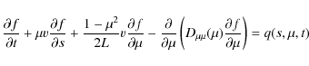
where s is the distance along the magnetic field line,
We used a Monte Carlo model to simulate the interplanetary transport of SEPs injected at the root of an Archimedean spiral magnetic field line (Agueda et al. 2008). Our calculations of the particle propagation were based on the focused transport model that includes the effects of adiabatic focusing by the diverging Parker field, the interplanetary scattering by magnetic fluctuations, and adiabatic deceleration resulting from the interplay of scattering and focusing (Ruffolo 1995; Kocharov et al. 1998). The results of the simulation give the directional distribution of particles at 1 AU, as a function of the time and energy range of interest.
As initial condition, we consider all particles to be injected
instantaneously at two solar radii from the center of the Sun. Thus,
the results of the simulation are expressed in terms of Green's
functions of particle transport. The energy spectrum of the solar
source is assumed to be a power law (
![]() )
with spectral index
)
with spectral index
![]() ,
which is estimated from the observational data (see Paper I).
,
which is estimated from the observational data (see Paper I).
In the solar wind frame, the pitch-angle diffusion coefficient can be expressed as
![]() ,
where
,
where ![]() is the scattering frequency and
is the scattering frequency and ![]() the particle pitch-angle cosine. We assume
the particle pitch-angle cosine. We assume
![]() ,
where
,
where ![]() allows us to simulate different scattering conditions, from quasi-isotropic (
allows us to simulate different scattering conditions, from quasi-isotropic (
![]() )
to fully anisotropic (
)
to fully anisotropic (
![]() ,
totally decoupled hemispheres in the
,
totally decoupled hemispheres in the ![]() -space). The scattering rate,
-space). The scattering rate, ![]() ,
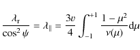
is determined from the mean free path parallel to the field
,
is determined from the mean free path parallel to the field
![]() or the radial mean free path
or the radial mean free path
![]() ,
which are related by (Hasselmann & Wibberenz 1968)
,
which are related by (Hasselmann & Wibberenz 1968)
|
(2) |
where v is the particle speed and
2.2 Fitting to sectored intensity profiles
For a given set of transport parameters (Thus, the goal is to solve the inversion problem of inferring the
transport parameters and the injection time profile at the Sun from a
set of in-situ measured sectored intensities Is(t), where Is(t) is the intensity measured at time t by sector s
in a given energy channel. By taking the angular response of the
sectors scanned by the LEFS60 telescope into account, we were able to
transform the simulated PADs into sectored intensities measured by the
telescope (see Paper I). The modeled sectored intensities,
![]() ,
in sector s can be written as
,
in sector s can be written as
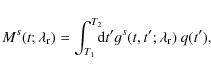
where q(t) - to be determined - represents the electron injection function and
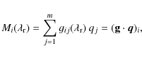
Considering the eight sectors of the telescope and discrete values of time, Eq. (3) can be written as
|
(4) |
where i=1,2,...,n numbers the total number of observational points;
The best-fit injection function,
![]() ,
can be determined by comparing the modeled intensities with the observations. Let b be the sector-averaged background intensity and
Ji=Ii-b. We want to derive the m-vector
,
can be determined by comparing the modeled intensities with the observations. Let b be the sector-averaged background intensity and
Ji=Ii-b. We want to derive the m-vector ![]() that minimizes the length of the
n-vector
that minimizes the length of the
n-vector
![]() ,
that means minimizing the value of
,
that means minimizing the value of
![]() subject to the constraint that
subject to the constraint that
![]()
![]() .
Thus, the best-fit injection function corresponds to a combination of m delta-function injection amplitudes at times tj.
To solve this inversion problem and obtain the best-fit injection
values, we use the non-negative least squares (NNLS) method of Lawson
& Hanson (1974).
.
Thus, the best-fit injection function corresponds to a combination of m delta-function injection amplitudes at times tj.
To solve this inversion problem and obtain the best-fit injection
values, we use the non-negative least squares (NNLS) method of Lawson
& Hanson (1974).
The best-fit transport parameters (
![]() and scattering case) are determined by minimizing the goodness-of-fit estimator
and scattering case) are determined by minimizing the goodness-of-fit estimator
The calculation of the goodness of the fit is restricted to the selected time interval. Each energy channel is separately fitted and the goodness-of-fit estimator of the whole fit is obtained by adding the values obtained for each energy channel.
3 NR electron events: observational characteristics
We considered eleven NR electron events observed by the LEFS60 telescope between 1998 and 2005 that meet the following criteria: (1) quietness in the interplanetary medium, with stable IMF and steady solar wind parameters from one hour prior to the onset of the event up to the end of the time interval selected for its simulation; (2) significant enhancement of NR electron intensities, i.e., spin-averaged peak intensities at least one order of magnitude higher than the pre-event background intensities in the E'4 energy channel; (3) negligible proton contamination in the electron energy channels of the LEFS60 telescope; and (4) good coverage in pitch-angle cosine of the electron distributions observed by the LEFS60 telescope.
Table 1 summarizes
the main characteristics of the selected NR electron events. The
first two columns list the name given to the event and the date when
the onset of the event was observed. The third column lists the time of
the onset of the event, t0, in the E'4 energy channel determined by means of the Poisson-CUSUM method (Huttunen-Heikinmaa et al. 2005).
The fourth column gives the rise time, i.e. the time interval between
the onset and the maximum, of the spin-averaged time-intensity profile
in the E'4 energy channel. The fifth column gives the time interval
selected for the study of each event. The next column lists the
strength, S, of the event defined as the logarithm of the ratio between the spin-averaged peak intensity, ![]() ,
and the spin-averaged mean intensity of the pre-event background,
,
and the spin-averaged mean intensity of the pre-event background, ![]() ,
in the E'4 energy channel; thus
,
in the E'4 energy channel; thus
![]() .
The seventh column lists the assumed spectral index of the injecting source (
.
The seventh column lists the assumed spectral index of the injecting source (
![]() ), estimated from the observed time-of-maximum differential intensity spectral index (see Paper I).
), estimated from the observed time-of-maximum differential intensity spectral index (see Paper I).
The mean pitch-angle cosine coverage of the LEFS60 telescope (
![]() )
is listed in the eighth column of Table 1. It is defined as the percentage of the pitch-angle cosine range scanned by the telescope; i.e.,
)
is listed in the eighth column of Table 1. It is defined as the percentage of the pitch-angle cosine range scanned by the telescope; i.e.,
|
(6) |
where
The velocity dispersion effect -understood as the fact that for an instantaneous injection at the Sun, the electron intensities at 1 AU should rise earlier at higher energy than at lower energies- is not clearly observed for most of the selected events, either because of the fluctuations in the background intensity or, in certain cases, secondary responses of the low-energy channels to higher-energy electrons (see Haggerty & Roelof 2002). An alternative method of proving the presence of velocity dispersion is to consider the onset time of the events at intensity levels that are a fixed percentage of the maximum intensity in each energy channel (Lintunen & Vainio 2004). Then, it becomes clear that all events but one (Jul00) show velocity dispersion. In this particular case, the lack of velocity dispersion indicates that the rising phase of the event might be compromised either because strong contributions from instrumental background or because a poor magnetic connection of the source to the observer masks the initial onset of the fluxes. If this was the case, the observer would see the onset of the event resulting from the evolution of the magnetic connection to the source rather than what results from a temporal increase of the fluxes inside a well-connected flux tube.
The selected events display a variety of rise times (see Table 1):
two events (May00 and Oct02) show a short rise time (<15 min),
while the others show longer rise times (up to 1 day). Since
we aim at characterizing the solar injection profile of the first
arriving electrons at 1 AU, we have chosen a period of
modelization that is a compromise between computing time requirements
and the validity of the scenario (injecting source close to the Sun,
stable IMF, and solar wind). The longest time period selected for
studying the events is four hours. The eleven events have S>1
and show, as a whole, a median event strength of 2.2 orders
of magnitude in the E'4 energy channel. The mean spectral index of the
source is
![]() .
Finally, all the events show a reasonably good coverage in pitch-angle cosine (
.
Finally, all the events show a reasonably good coverage in pitch-angle cosine (
![]() %) that qualifies them for study.
%) that qualifies them for study.
Our model assumes the Parker model of the IMF. In this model, the path length and the nominal footpoint of the field line connecting the observer to the Sun are determined by the solar wind speed. Columns 9 and 10 of Table 1 give the mean value of the solar wind speed measured from one hour prior to the onset of the event up to the end of the period considered and the longitude of the corresponding nominal footpoint of the IMF line connecting the observer with the Sun. Stable solar wind speeds ranging from 300 to 700 km s-1, with a mean standard deviation below 4%, are observed in the selected time intervals.
Columns 11-14 of Table 1 give the characteristics of the IMF at 1 AU: the mean latitude,
![]() ,
and longitude,
,
and longitude,
![]() ,
of the IMF in the geocentric solar ecliptic (GSE) coordinate system, as
well as the value of the modal polarity of the IMF and its prevailing
period percentage. We define the polarity of the interplanetary
magnetic field as
,
of the IMF in the geocentric solar ecliptic (GSE) coordinate system, as
well as the value of the modal polarity of the IMF and its prevailing
period percentage. We define the polarity of the interplanetary
magnetic field as
where BR and BT are the R and T components of the magnetic field vector in the radial tangential normal (RTN) coordinate system, respectively. As can be seen, the magnetic field orientations have a standard deviation of less than 50
Figure 1 shows the
spin-averaged 62-312 keV electron intensities observed by the
EPAM/LEFS60 telescope for ten of the events under study. The gray area
shows the studied time period; as listed in Table 1.
For each event, the upper panel includes the electron intensities
observed by the E' channels (thick curve) and the DE channels
(thin curve) in approximately the same energy range. The similar
trends, during the selected time periods, suggest that there is
negligible ion contamination in the studied LEFS60 electron
intensities. For each event in Fig. 1, the four lower panels show the solar wind speed and the IMF magnitude and direction (where ![]() is the latitude and
is the latitude and ![]() is the longitude in the GSE coordinate system).
is the longitude in the GSE coordinate system).
![\begin{figure}
\par\includegraphics[angle=90,width=17cm,clip]{12224fg1.eps}
\end{figure}](/articles/aa/full_html/2009/44/aa12224-09/img107.png)
|
Figure 1:
Electron events. For each event and from top to bottom:
electron spin-averaged intensities observed by the LEFS60 telescope in
three different energy channels E'2 62-102 keV, E'3
102-175 keV, and E'4 175-312 keV (thick); deflected electron
intensities in approximately the same energy ranges: DE2
53-103 keV, DE3 103-175 keV, and DE4 175-315 keV (thin).
Solar wind speed observed by ACE/SWEPAM. Magnetic field magnitude, latitude ( |
| Open with DEXTER | |
4 Associated electromagnetic emissions
We used observations reported by the Solar Geophysical Data (SGD; US Department of Commerce, Boulder, CO, USA)![]() to identify both the H
to identify both the H![]() flares associated with the origin of each NR electron event and
the characteristics of the soft X-ray (SXR) event observed by the GOES
satellite in the 1-8 Å band. In addition, we included hard X-ray
(HXR) observations from the Hard X-ray Telescope (Kosugi et al. 1991) onboard Yohkoh and from the Reuven Ramaty High-Energy Solar Spectroscopic Imager (RHESSI; Lin et al. 2002), whenever available. We also utilize 14 MHz-20 kHz radio data acquired by the WAVES experiment on the Wind spacecraft (Bougeret et al. 1995)
flares associated with the origin of each NR electron event and
the characteristics of the soft X-ray (SXR) event observed by the GOES
satellite in the 1-8 Å band. In addition, we included hard X-ray
(HXR) observations from the Hard X-ray Telescope (Kosugi et al. 1991) onboard Yohkoh and from the Reuven Ramaty High-Energy Solar Spectroscopic Imager (RHESSI; Lin et al. 2002), whenever available. We also utilize 14 MHz-20 kHz radio data acquired by the WAVES experiment on the Wind spacecraft (Bougeret et al. 1995)![]() .
The spectral plots allow us to estimate the start and end times of the
radio bursts measured at 14 MHz observed in association with the
electron events, to the nearest 5 minutes. Finally, we used white light
observations of CMEs from LASCO (Brueckner et al. 1995)
and obtain the characteristics (speed, width and time) of the CMEs
observed in association with the NR electron events from the SOHO/LASCO CME catalog (Yashiro et al. 2004)
.
The spectral plots allow us to estimate the start and end times of the
radio bursts measured at 14 MHz observed in association with the
electron events, to the nearest 5 minutes. Finally, we used white light
observations of CMEs from LASCO (Brueckner et al. 1995)
and obtain the characteristics (speed, width and time) of the CMEs
observed in association with the NR electron events from the SOHO/LASCO CME catalog (Yashiro et al. 2004)![]() . Associations are made primarily on the basis of location and timing information.
. Associations are made primarily on the basis of location and timing information.
Table 2 summarizes
the properties of the electromagnetic emissions observed in association
with the selected NR electron events. The first column gives the
date of the event, the following three columns give the characteristics
of the SXR flare (start time, rise time, and class). Columns 5-8
give the characteristics of the H![]() flare (start time, rise time, importance, and location). The next
column gives the absolute value of the difference between the
heliolongitude of the H
flare (start time, rise time, importance, and location). The next
column gives the absolute value of the difference between the
heliolongitude of the H![]() flare and the longitude of the nominal Parker spiral magnetic field
line footpoint connecting the spacecraft with the Sun (listed in
Table 1).
Columns 10 and 11 give the characteristics of the HXR
emission (start time and duration). Column 12 gives the estimated
duration of the associated type III radio bursts at 14 MHz.
Columns 13-17 list the parameters of the associated CMEs as
reported in the SOHO/LASCO
CME catalog: (13), (14) the time and height of the CME at the
first appearance in the C2 coronograph, (15) the position angle
(PA, measured counterclockwise from the conventional solar north),
(16) the plane-of-sky speed of the leading-edge and (17) the
angular width. The last column quotes previous works that have made the
same association between flare/CME and particle event.
flare and the longitude of the nominal Parker spiral magnetic field
line footpoint connecting the spacecraft with the Sun (listed in
Table 1).
Columns 10 and 11 give the characteristics of the HXR
emission (start time and duration). Column 12 gives the estimated
duration of the associated type III radio bursts at 14 MHz.
Columns 13-17 list the parameters of the associated CMEs as
reported in the SOHO/LASCO
CME catalog: (13), (14) the time and height of the CME at the
first appearance in the C2 coronograph, (15) the position angle
(PA, measured counterclockwise from the conventional solar north),
(16) the plane-of-sky speed of the leading-edge and (17) the
angular width. The last column quotes previous works that have made the
same association between flare/CME and particle event.
All the selected electron events are clearly associated with
intense SXR flares of variable duration. Eight events are associated
with a single active region, while three events (May98, Oct02, and
Dec02) are associated with two western active regions. The difference
in heliolongitudes between the H![]() flare and the nominal footpoint of the IMF line connecting to the spacecraft,
flare and the nominal footpoint of the IMF line connecting to the spacecraft, ![]() ,
is less than
,
is less than ![]() in all events.
in all events.
All the selected electron events are preceded by type III radio bursts.
These bursts are the dominant feature of the radio dynamic spectrum of
the day in most cases. Most of the NR electron events are
associated with a CME observed by LASCO; with the exception the Jun05
event because there were no LASCO CME observations available. As can be
seen in Table 2, the associated CMEs were first observed after the start of the SXR event, typically by ![]() 10 to 60 min; note that the height of the CMEs was already 3.5-6
10 to 60 min; note that the height of the CMEs was already 3.5-6 ![]() .
In one case (Sep04), the CME was first observed in the C3 coronograph
images about five hours after the start of the SXR event; when the CME
was already above
.
In one case (Sep04), the CME was first observed in the C3 coronograph
images about five hours after the start of the SXR event; when the CME
was already above ![]() 31
31 ![]() .
All the CMEs were seen to propagate mostly out of the west limb with high plane-of-sky velocities (
.
All the CMEs were seen to propagate mostly out of the west limb with high plane-of-sky velocities (![]() 850 km s-1). Eight of them (May98, Jul00, Nov00, Apr01, Dec01, Aug02, Dec02 and Sep04) have angular widths larger than
850 km s-1). Eight of them (May98, Jul00, Nov00, Apr01, Dec01, Aug02, Dec02 and Sep04) have angular widths larger than ![]() 100
100![]() ;
whereas two events (May00 and Oct02) were associated with narrow (<
;
whereas two events (May00 and Oct02) were associated with narrow (<![]() )
CMEs.
)
CMEs.
5 Results and discussion
5.1 Simulation of the NR electron events
We simulated the NR electron events following the same procedure
as described in Paper I for the May00 event. We consider three
scattering cases: isotropic scattering (
![]() )
and two
)
and two ![]() -dependent scattering cases, one with
-dependent scattering cases, one with
![]() and one with
and one with
![]() ,
for several values of
,
for several values of
![]() ,
quasi-logarithmically spaced between 0.04 AU and 1.5 AU.
,
quasi-logarithmically spaced between 0.04 AU and 1.5 AU.
Table 3 shows
the results obtained for the selected events. The first column lists
the name of the event, the next three columns give the goodness-of-fit
estimator, ![]() (cf. Eq. (5)). For each scattering case: (1) isotropic; (2)
(cf. Eq. (5)). For each scattering case: (1) isotropic; (2) ![]() -dependent with
-dependent with
![]() ;
and (3)
;
and (3) ![]() -dependent with
-dependent with
![]() ,
respectively. In all cases,
,
respectively. In all cases, ![]() shows a minimum around the best-fit
shows a minimum around the best-fit
![]() value. For each scattering case, the optimal
value. For each scattering case, the optimal
![]() values are listed in the three subsequent columns (best-fit values are
indicated in bold). The scattering case that shows the lowest
values are listed in the three subsequent columns (best-fit values are
indicated in bold). The scattering case that shows the lowest ![]() is listed in the last column of Table 3.
For two events, we obtained
is listed in the last column of Table 3.
For two events, we obtained
![]() AU, while for the other nine
AU, while for the other nine
![]() AU. According to the values of the goodness of fit estimator, eight of the events can be best fitted assuming
AU. According to the values of the goodness of fit estimator, eight of the events can be best fitted assuming ![]() -dependent scattering and three events assuming isotropic pitch-angle scattering.
-dependent scattering and three events assuming isotropic pitch-angle scattering.
Table 2: Electromagnetic emissions associated with the electron events.
![\begin{figure}
\par\includegraphics[width=12cm,clip]{12224fg2.eps}
\end{figure}](/articles/aa/full_html/2009/44/aa12224-09/img118.png)
|
Figure 2:
NR electron event on 2001 Dec. 26 as observed by the
LEFS60 telescope. Electron sectored intensities E'4 175-312 keV,
E'3 102-175 keV ( |
| Open with DEXTER | |
Table 3:
Goodness-of-fit estimator ![]() and radial mean free path obtained for each scattering case: (1) isotropic; (2)
and radial mean free path obtained for each scattering case: (1) isotropic; (2) ![]() -dependent with
-dependent with
![]() ;
and (3)
;
and (3) ![]() -dependent with
-dependent with
![]() ,
and the scattering case giving the lowest
,
and the scattering case giving the lowest ![]() .
.
Earlier studies utilizing low-order Legendre expansions of the PAD (e.g., Beeck & Wibberenz 1986; Hatzky et al. 1995; Hatzky & Wibberenz 1995)
have shown that it is possible to determine the value of the mean free
path from fitting the evolution of the first-order anisotropy alone,
but only higher-order anisotropies provide information about the
detailed shape of the pitch-angle diffusion coefficient. By fitting the
intensities observed in eight different sectors, we acquire the maximal
amount of directional information of the particle distribution present
in the data, and if the angular coverage of the sectors is good, the
equivalent amount of Legendre coefficients is relatively high. As can
be seen in Table 3, the
best-fit values of the radial mean free path are nearly independent of
the shape of the adopted pitch-angle diffusion coefficient, which is
consistent with the earlier studies cited above. However, the small
differences within the ![]() -values
are enough to allow us to determine the best-fit form of the diffusion
coefficient, among the three scattering models. It is important to note
that the adopted scattering model can affect the shape and timing of
the injection profile of particles at the Sun (see Agueda 2008)
and, although the value of the mean free path may be fitted correctly
even with an incorrect form of the diffusion coefficient, the injection
profile derived gets distorted.
-values
are enough to allow us to determine the best-fit form of the diffusion
coefficient, among the three scattering models. It is important to note
that the adopted scattering model can affect the shape and timing of
the injection profile of particles at the Sun (see Agueda 2008)
and, although the value of the mean free path may be fitted correctly
even with an incorrect form of the diffusion coefficient, the injection
profile derived gets distorted.
We have considered the same scattering model for all electron
energies and throughout the time period studied in each event. If we
would allow the scattering case to vary from one energy channel to
another, we would have obtained even lower values of ![]() .
The general trend seems to be that the best fit case is more isotropic
at low energies than at high energies. The differences, however, are
too small for a detailed analysis.
.
The general trend seems to be that the best fit case is more isotropic
at low energies than at high energies. The differences, however, are
too small for a detailed analysis.
Figure 2 shows the
best fit for the Dec01 event. Panels 1 to 8 display the observed (color
dots) and modeled (black curves) intensities in each sector of the
LEFS60 telescope (top) for three energy channels (E'2, E'3, E'4) and
the pitch-angle cosine (![]() )
range scanned by each sector (bottom) through the time interval selected for simulation. Figure 3
sketches the solid angle encompassed by the LEFS60 telescope projected
onto a sphere and the approximate definition of the sectors. As can be
seen from Fig. 3, a change in the direction of the magnetic field vector produces a change in the
)
range scanned by each sector (bottom) through the time interval selected for simulation. Figure 3
sketches the solid angle encompassed by the LEFS60 telescope projected
onto a sphere and the approximate definition of the sectors. As can be
seen from Fig. 3, a change in the direction of the magnetic field vector produces a change in the ![]() -range swept by each sector. Figure 2
shows the time evolution of the pitch-angle cosine of the particles
getting in the detector along the midpoint clock-angle zenith direction
of the sector, whereas the gray area shows the pitch-angle cosine range
scanned by the sector as a function of time. The last panel in
Fig. 2 displays the
omni-directional intensities (top) and the evolution of the mean
pitch-angle cosine (bottom) deduced from the model. The gray area
displays the range of pitch-angle cosines scanned by the LEFS60
telescope as a function of time.
-range swept by each sector. Figure 2
shows the time evolution of the pitch-angle cosine of the particles
getting in the detector along the midpoint clock-angle zenith direction
of the sector, whereas the gray area shows the pitch-angle cosine range
scanned by the sector as a function of time. The last panel in
Fig. 2 displays the
omni-directional intensities (top) and the evolution of the mean
pitch-angle cosine (bottom) deduced from the model. The gray area
displays the range of pitch-angle cosines scanned by the LEFS60
telescope as a function of time.
The best-fit transport parameters for the Dec01 event are
![]() AU for a pitch-angle dependent scattering model with
AU for a pitch-angle dependent scattering model with
![]() .
The fit succeeds in reproducing most of the features of the intensity
profiles (data marked with blue dots are not taken into account in the
fit due to a reversal of the IMF polarity). Small differences between
observational and simulated sectored intensities are observed during
these changes of polarity in the IMF and indicate that the injection
history and/or the interplanetary transport conditions of
NR electrons were similar in the flux tubes with opposite
polarity.
.
The fit succeeds in reproducing most of the features of the intensity
profiles (data marked with blue dots are not taken into account in the
fit due to a reversal of the IMF polarity). Small differences between
observational and simulated sectored intensities are observed during
these changes of polarity in the IMF and indicate that the injection
history and/or the interplanetary transport conditions of
NR electrons were similar in the flux tubes with opposite
polarity.
It is important to note that the wiggles in the sectored intensity profiles are observed under rather stable conditions of the omni-directional intensities and the first-order anisotropy, because they result from fluctuations of the interplanetary magnetic field direction that make a given sector scan different parts of the electron pitch-angle distribution. The modeled intensities are able to follow the wiggles because the changes of the local direction of the magnetic field are taken into account in the modelization. In some cases, some fluctuations in the observed intensity profiles may be caused by crossings of magnetic flux tubes with different transport conditions; this effect cannot be taken into account in our model.
The fits of the other events also succeed in reproducing most
of the features of the observational intensity profiles in the eight
different sectors. Figure 4 shows the best-fit time-intensity profiles for nine of the events modeled in the present paper. For each event, Fig. 4
displays the two sectors scanning particles propagating mainly sunward
and antisunward along the magnetic field direction, in the same
presentation as in Fig. 2.
Five of the events (May98, Nov00, Aug02, Oct02 and Jun05) show
discrepancies between the observed and modeled profiles in those
sectors scanning mainly particles coming sunward. For the Nov00 and
Oct02, the discrepancies between the simulated and the observed
sectored intensities are greater in the low energy channel and the
sectors scanning particles coming mainly in the sunward direction. The
modeled intensities are higher than observations in these sectors,
showing underpredicted anisotropies in the beginning of the event,
which suggests that for these events the model overestimates the
scattering processes at work. Thus, scattering models with a wider
resonance gap near ![]() or with spatially varying
or with spatially varying ![]() ,
for example, might perform better for these events.
,
for example, might perform better for these events.
![\begin{figure}
\par\includegraphics[width=6.5cm,clip]{12224fg3.eps}
\end{figure}](/articles/aa/full_html/2009/44/aa12224-09/img124.png)
|
Figure 3:
Solid angle encompassed by the LEFS60 telescope projected onto a
sphere. In the spacecraft coordinate system, z is the spacecraft
spin axis and the x-y plane is perpendicular to it. |
| Open with DEXTER | |
In the case of the May98 event, the optimum fit succeeds in reproducing the sector profiles during the rising phase of the event. However, just after the peak intensity the simulation slightly underestimates the intensities observed in the sectors observing particles mainly propagating toward the Sun. The analysis of suprathermal (210 eV) electron PADs observed by Wind (not shown here) reveals bidirectional electron streams during the decay phase of this event. No interplanetary CME (ICME) signatures were observed during the event time interval. The solar wind ion charge states were inconsistent with the presence of an interplanetary CME; the magnetic field did not show a smooth evolution of magnitude, and orientation; additionally, there were no halo/partial halo CMEs before the selected time period. Therefore, the disagreement in the fit during an extended time period after the maximum is probably related to the fact that the model assumes that the IMF is a Parker spiral, while a detailed analysis of the interplanetary conditions indicates a more complex scenario. This is also the case for the Aug02 and Jun05 events that were preceded by ICMEs: the Aug02 event occurs during a very small magnetic loop and the Jun05 event shows counterstreaming electrons at suprathermal energies that might stem from a corrotating interaction region. In any case, the relatively good agreement between the model and the observations suggests that the Parker IMF model is a valid assumption to get a picture of the injection function of the first arriving particles.
5.2 Comparison of solar NR electron injection profiles with electromagnetic emissions
Figure 5 shows the best-fit injection function (top panel) and the timing of the associated electromagnetic emissions for the Dec01 event: i.e. the soft X-ray emission (middle panel) and the radio emission observed by Wind/WAVES (bottom panel), together with the frequency of emission of the plasma at the the height of the CME leading-edge if the density model of Vrsnak et al. (2004) is used. There were no hard X-ray observations during this event. For the sake of comparison with the electromagnetic emissions, the electron injection times are shifted by 8.3 min to account for the light travel time.
The inferred injection profile shows a single component starting at 05:20 UT, nearly simultaneous in the three energy channels (E'2, E'3, and E'4), and lasting at least three hours. The injection profile appears patchy, however, if we convolve the modeled Green's functions by a smoothed injection profile (see smoothed curves in Fig. 5, calculated using a 6-point moving average), the fit does not differ from the best fit. Part of this patchiness could be related to how the deconvolution procedure may try to fit statistical fluctuations and/or effects of magnetic flux tube crossings in the intensity measurements (see Agueda 2008). In extreme cases, this can produce spurious injection episodes.
The beginning of the NR electron injection coincides with the beginning of a type II radio burst (see Cane & Erickson 2005). The observed radio emission is consistent with its origins in a source located behind the CME leading edge, assuming the density model of Vrsnak et al. (2004) (Fig. 5). However, the high frequency may also result from an overdense coronal/interplanetary structure emitting the radio burst.
The 102-175 keV injection profiles inferred for the other nine events and the timing of their associated electromagnetic emissions are shown in Fig. 6. In this set of eleven events we identify two types of episodes in the inferred injection profiles: short (<15 min) and time-extended (>1 h). Both episodes can coexist in the same time profile. The injection profiles of the May00, Jul00 and Oct02 events show two injection episodes separated by 30 min on average: an initial injection episode of short duration, followed by a delayed much longer lasting episode (>1 h). The injection profiles of the Nov00, Dec01, Aug02 and Sep04 events display time-extended injection components. The May98 event shows an injection profile composed of only a main short injection episode, whereas for the Apr01, Dec02, and Jun05 events the first short episodes are followed by several sparse short injection episodes. In seven events, the injection takes place first at low energies (E'2 channel) but the differences with the other energy channels (E'3 and E'4 channels) are always less than 5 min.
At low energies (62-102 keV), small injection episodes preceding the main injection episode are observed, for example in the Jul00 and Oct02 events, that could be related to secondary responses of the E'2 energy channel. Haggerty & Roelof (2006) determine the response function of the EPAM deflected electron channels and find that DE2 (53-103 keV) and DE3 (103-175 keV) channels can have strong responses to electrons of energies >250 keV in addition to electrons of their nominal energies. These secondary responses would move the onset time of the event to earlier times than if the detectors collected only electrons within the prescribed energy range (with the strongest effect being observed in the DE2 channel), but their effects would not be noticeable right before, during, or after the time of maximum intensity, as long as the injection spectrum is not abnormally hard (Haggerty & Roelof 2006).
Ideally, the true energy response of the channels, together with the angular response of the sectors, would have to be utilized to accurately deconvolve in-situ particle measurements. The energy response of the LEFS60 electron channels is not considered here because to our knowledge, no previous study has quantified it yet. We did, however, perform a simplified study to estimate the effect of secondary responses in the inferred injection profile. We generated a simulated data set assuming that electrons at energies nominally in the E'3 and E'4 channels contribute a background to the E'2 channel at levels similar to the secondary responses of the EPAM DE2 channel reported by Haggerty & Roelof (2006). We then deconvolved the simulated E'2 intensity (as described in Sect. 2) assuming only the nominal energy response of the channel. We found that the secondary responses result in small false precursors in the injection profiles that shift the beginning of the inferred injection to earlier times. The timing of the maximum injection, however, is not affected by the secondary responses, because typical injection spectra decrease rather steeply as a function of energy.
![\begin{figure}
\par\includegraphics[width=16cm,clip]{12224fg4.eps}
\end{figure}](/articles/aa/full_html/2009/44/aa12224-09/img125.png)
|
Figure 4:
For each event ( from top to bottom):
electron sectored intensities observed by the LEFS60 telescope in the
sector scanning particles coming mainly field aligned along the
antisunward direction in the E'4, E'3, and E'2 energy channels
(the black curves show the modeled sectored intensities, the red dots
the observational data, and the blue dots periods associated with
reversals of the IMF polarity); pitch-angle cosine, |
| Open with DEXTER | |
Table 4:
Derived injection components at ![]() 80 keV.
80 keV.
For all the events, the onset of the derived injection profiles occurs
within the rising phase or near the maximum of the soft X-ray emission,
with the following components developing at or after the time of the
SXR peak. At low energies (E'2), the peak of the first short injection
episode coincides with the onset of the type III radio emission.
For four of the events (May00, Jul00, Apr01 and Dec02), the radio
emission is accompanied by HXR emission that peaks in coincidence with
the first electron injection episode. On the other hand, some of the
delayed injection episodes seem to be related to intermittent radio
emissions at the height of the CME leading edge (see May00, Jul00, and
Oct02 events). For the Dec02, Jun05, and Apr01, the injection episodes
observed after the main injection episode are short and sparse. For the
Apr01 and Dec02 events these injection episodes coincide with the
observation of radio emission coming from heights below the CME leading
edge. The injection profile of four of the events (Nov00, Dec01, Aug02,
and Sep04) shows no prompt injection episode. In these cases, the
timing of the injection correlates with type II radio bursts; all
of them listed in the Wind/WAVES web site![]() .
.
![\begin{figure}
\par\includegraphics[width=7cm,clip]{12224fg5.eps}
\end{figure}](/articles/aa/full_html/2009/44/aa12224-09/img150.png)
|
Figure 5: Electron injection profiles derived for the three modeled energy channels (injection times are shifted by 8.3 min to account for the light travel time): E'2, E'3, and E'4 - in addition to the fit result (histogram), smoothed curves obtained by six-point moving averaging are shown -, along with the soft X-ray flux observed by GOES in W/m2, the radio flux (in dB over background) observed by Wind, and the local electron plasma frequency at the height of the CME leading edge (dotted curve). |
| Open with DEXTER | |
Table 4 lists the
properties of the prompt and delayed injection components identified in
the lowest energy channel (E'2; 62-102 keV). The first column
gives the date of the event. The second column lists the injection
time-integrated spectral index,
![]() ,
deduced by integrating the injection function over time for each energy
channel (see Paper I). These values are similar to those estimated
from observations (Table 1).
The following four columns give, for the identified prompt short
injection episodes, the onset, duration, number of particles
(in e sr-1 MeV-1), and percentage
of the total injection. The number of particles is given per unit solid
angle at the solar-wind source surface, so the total number of
accelerated particles would be given by multiplying this number by the
solid angle covered by those flux tubes that are populated by the
accelerated electrons. The last three columns in Table 4 give the onset, duration, and injection rate (in e sr-1 MeV-1 s-1) of the delayed episodes.
,
deduced by integrating the injection function over time for each energy
channel (see Paper I). These values are similar to those estimated
from observations (Table 1).
The following four columns give, for the identified prompt short
injection episodes, the onset, duration, number of particles
(in e sr-1 MeV-1), and percentage
of the total injection. The number of particles is given per unit solid
angle at the solar-wind source surface, so the total number of
accelerated particles would be given by multiplying this number by the
solid angle covered by those flux tubes that are populated by the
accelerated electrons. The last three columns in Table 4 give the onset, duration, and injection rate (in e sr-1 MeV-1 s-1) of the delayed episodes.
For most of the events, the number of particles injected during the
first short injection episode represents more than 50% of the total
injection. The exception are those events without the first short
injection episode (Nov00, Dec01, Aug02, and Sep04) and the Jul00 event
where the first episode injects only 33% of the total amount of
particles injected during the studied period. In this case, that the
electron intensities increased a factor of 5 in the following day (see
Fig. 3 in Smith et al. 2001)
suggests that the delayed injection is not complete at the end of the
time interval selected here to study and that this percentage would
have been lower if the studied period had been extended. In our model
the source of particles is assumed to be fixed in the corona. However,
the motion of the source should be taken into account if it is related
to a CME-driven shock and one aims to study the events for a long time
period. In the present study we have neglected this motion because the
observed CMEs did not travel far from the Sun (<30 ![]() )
during the modeled periods, so the release of NR electrons can be considered as happening close to the Sun.
)
during the modeled periods, so the release of NR electrons can be considered as happening close to the Sun.
![\begin{figure}
\par\includegraphics[width=15cm,clip]{12224fg6.eps}
\end{figure}](/articles/aa/full_html/2009/44/aa12224-09/img151.png)
|
Figure 6: Electron injection profiles derived in the E'3 energy range and associated electromagnetic emissions (same presentation as in Fig. 5). |
| Open with DEXTER | |
Figure 7 (top) shows the number of particles, ![]() (in e sr-1 MeV-1), injected during the short injection episodes as a function of the intensity of the associated SXR flare, Ix (in W m-2). The error in
(in e sr-1 MeV-1), injected during the short injection episodes as a function of the intensity of the associated SXR flare, Ix (in W m-2). The error in ![]() has been estimated by calculating the total number of particles
injected during the short injection episode if the two values of
has been estimated by calculating the total number of particles
injected during the short injection episode if the two values of
![]() closest to the best fit case are assumed. As can be seen, the higher
the intensity of the SXR flare, the higher the number of
NR electrons injected. A linear fit to these points yields
closest to the best fit case are assumed. As can be seen, the higher
the intensity of the SXR flare, the higher the number of
NR electrons injected. A linear fit to these points yields
with correlation coefficient 0.946. To firmly establish a relation of this type, it would be necessary to include more NR electrons events in the sample, especially those associated with X-class X-ray flares.
Figure 7 (bottom)
shows the injection rate of the delayed injection episodes as a
function of the plane-of-sky speed of the associated CME-leading edge.
It also shows the error in the estimation of the CME-leading edge speed
and the error in the injection rate of the delayed injection episodes,
which is estimated, as before, by calculating its value for the two
values of
![]() closest to the best fit case. If we only take into account the data
points corresponding to those events that show a delayed time-extended
injection component, we do not find a clear correlation between the
injection rate of particles and the speed of the associated CME
leading-edge (correlation coefficient 0.791), because the
injection rate can depend on variables not considered here such as the
actual speed of the coronal shock (not affected by projection effects),
the kinetic energy of the CME, and/or the time evolution of the
CME-driven shock. The injection rates of the delayed component of the
Apr01 and Jun05 events denoted by stars in Fig. 7
(bottom) are not taken into account in the fit. Their sparse occurrence
suggests that they could be related to magnetic restructuring processes
happening in the aftermath of the CME leading-edge, as suggested by the
coincidence of the injection episodes and the radio emission observed
from heights from behind the CME leading-edge. Therefore, both coronal
shocks and reconnection processes seem to play a role in the injection
of NR electrons.
closest to the best fit case. If we only take into account the data
points corresponding to those events that show a delayed time-extended
injection component, we do not find a clear correlation between the
injection rate of particles and the speed of the associated CME
leading-edge (correlation coefficient 0.791), because the
injection rate can depend on variables not considered here such as the
actual speed of the coronal shock (not affected by projection effects),
the kinetic energy of the CME, and/or the time evolution of the
CME-driven shock. The injection rates of the delayed component of the
Apr01 and Jun05 events denoted by stars in Fig. 7
(bottom) are not taken into account in the fit. Their sparse occurrence
suggests that they could be related to magnetic restructuring processes
happening in the aftermath of the CME leading-edge, as suggested by the
coincidence of the injection episodes and the radio emission observed
from heights from behind the CME leading-edge. Therefore, both coronal
shocks and reconnection processes seem to play a role in the injection
of NR electrons.
![\begin{figure}
\par\includegraphics[width=7cm,clip]{12224fg7.eps}
\end{figure}](/articles/aa/full_html/2009/44/aa12224-09/img154.png)
|
Figure 7: Top panel: number of particles injected during the prompt injection component in the E'2 (62-102 keV) energy channel versus the intensity of the associated soft X-ray flare. Bottom panel: injection rate of the delayed injection component versus the CME leading-edge speed; data from the Apr01 and Dec02 events is denoted by a star and is not included in the fit (see text for details). |
| Open with DEXTER | |
5.3 Comparison with other studies
Three of the events studied in this paper (May00, Jul00, and Apr01)
have already been modeled in previous works. Kartavykh et al. (2007) modeled the May00 electron event observed by Wind/3DP. They fitted the 40 keV electron time-intensity and anisotropy profiles and obtained
![]() AU.
The injection function was determined by varying its shape through a
number of grid points and performing a linear interpolation between
them according to the time resolution of the fit. The fit is consistent
with a single injection episode starting at 10:14 UT and reaching
a maximum at 10:24 UT. We obtained
AU.
The injection function was determined by varying its shape through a
number of grid points and performing a linear interpolation between
them according to the time resolution of the fit. The fit is consistent
with a single injection episode starting at 10:14 UT and reaching
a maximum at 10:24 UT. We obtained
![]() AU
and an injection profile composed of a prompt, short episode (with the
peak of the injection occurring at 10:20 UT), followed by a
delayed time-extended one (see Paper I) from fitting the sectored
intensities observed by ACE. In principle, the method of Kartavykh et al. (2007)
is able to capture several different injection components, but from the
comparison to the timing of our derived injection profile it seems that
the time resolution employed by them was not enough to resolve the two
components. Furthermore, Wind and ACE were separated by more than 106 km,
and it could be possible that quite different propagation conditions
prevailed in the flux tubes connected to the spacecraft. The 3DP
experiment onboard the Wind spacecraft (Lin et al. 1995)
is able to provide a three-dimensional coverage of the directional
particle distribution and therefore allows detailed study of the PADs.
AU
and an injection profile composed of a prompt, short episode (with the
peak of the injection occurring at 10:20 UT), followed by a
delayed time-extended one (see Paper I) from fitting the sectored
intensities observed by ACE. In principle, the method of Kartavykh et al. (2007)
is able to capture several different injection components, but from the
comparison to the timing of our derived injection profile it seems that
the time resolution employed by them was not enough to resolve the two
components. Furthermore, Wind and ACE were separated by more than 106 km,
and it could be possible that quite different propagation conditions
prevailed in the flux tubes connected to the spacecraft. The 3DP
experiment onboard the Wind spacecraft (Lin et al. 1995)
is able to provide a three-dimensional coverage of the directional
particle distribution and therefore allows detailed study of the PADs.
Bieber et al. (2001) simulated the Jul00 particle event observed by Wind
assuming a magnetic compression beyond the Earth resulting from an
earlier CME that passed eastward of Earth. They succeed in reproducing
the intensities and anisotropies observed during the ![]() 2 GeV proton event but not during the simultaneous 27-179 keV electron event. Bieber et al. (2001) tried to model the electron event out to about 11:00 UT. We extended the fit until 13:30 UT. They obtained
2 GeV proton event but not during the simultaneous 27-179 keV electron event. Bieber et al. (2001) tried to model the electron event out to about 11:00 UT. We extended the fit until 13:30 UT. They obtained
![]() AU
for the 27 keV electrons and 0.36 AU for the 179 keV
electrons. They pointed out that the fit becomes difficult after
11:00 UT because of a possible second injection component. Our
model is able to fit the electron sectored intensities for a longer
period of time without the assumption of a reflecting barrier beyond
the Earth, and it is consistent with
AU
for the 27 keV electrons and 0.36 AU for the 179 keV
electrons. They pointed out that the fit becomes difficult after
11:00 UT because of a possible second injection component. Our
model is able to fit the electron sectored intensities for a longer
period of time without the assumption of a reflecting barrier beyond
the Earth, and it is consistent with
![]() AU and two electron injection episodes.
AU and two electron injection episodes.
Maia et al. (2007) modeled the 178-290 keV electron intensities observed by ACE during the Apr01 event using a two-step procedure to infer the injection function and the value of
![]() :
first they infer the injection function by deconvolving the omni-directional intensities and then determine
:
first they infer the injection function by deconvolving the omni-directional intensities and then determine
![]() by minimizing the squared differences between the observed and modeled first order anisotropies. Maia et al. (2007) obtain
by minimizing the squared differences between the observed and modeled first order anisotropies. Maia et al. (2007) obtain
![]() AU
and infer a short (<10 min) injection of electrons with the
bulk of the particles being released around 13:50 UT. There are
several differences between our model and the model developed by Maia
et al. (2007). First of all, they assume isotropic pitch-angle scattering, while in our transport model we allow for
AU
and infer a short (<10 min) injection of electrons with the
bulk of the particles being released around 13:50 UT. There are
several differences between our model and the model developed by Maia
et al. (2007). First of all, they assume isotropic pitch-angle scattering, while in our transport model we allow for ![]() -dependent
pitch-angle scattering. In addition, they infer the injection function
and the transport conditions using omni-directional intensities and the
first-order anisotropy, while we use all the directional information
contained in the observational sectored intensities. Furthermore, in
the deconvolution method used by Maia et al. (2007),
the injection function is not constrained to be positive. Finally, the
goodness of the fit is defined by two different estimators in the two
models. Nevertheless, if we assume the best-fit transport conditions
inferred by Maia et al. (2007) (
-dependent
pitch-angle scattering. In addition, they infer the injection function
and the transport conditions using omni-directional intensities and the
first-order anisotropy, while we use all the directional information
contained in the observational sectored intensities. Furthermore, in
the deconvolution method used by Maia et al. (2007),
the injection function is not constrained to be positive. Finally, the
goodness of the fit is defined by two different estimators in the two
models. Nevertheless, if we assume the best-fit transport conditions
inferred by Maia et al. (2007) (
![]() AU
and isotropic scattering), we obtain that the best-fit injection
function at 175-312 keV is a delta function peaking at the same
time as the injection profile deduced by Maia et al. (2007). Our model, however, shows a significantly better fit for
AU
and isotropic scattering), we obtain that the best-fit injection
function at 175-312 keV is a delta function peaking at the same
time as the injection profile deduced by Maia et al. (2007). Our model, however, shows a significantly better fit for
![]() AU, leading us to conclude that the event has a delayed injection component, as also indicated by the radio emission.
AU, leading us to conclude that the event has a delayed injection component, as also indicated by the radio emission.
6 Summary and conclusions
We have studied eleven NR electron events observed by the LEFS60 telescope of the EPAM instrument on ACE between 1998 and 2005 with the aim of estimating the roles that solar flares, CME-driven shocks, and processes of magnetic restructuring in the aftermath of the CMEs play in the injection of NR electrons. To correctly infer the histories of the NR electron injections it is necessary to properly model the transport conditions of NR electrons along the IMF lines and to make complete use of the directional information contained in the in-situ particle data.
For most of the events, we were able to reproduce the observed
sectored intensities. In three cases (May98, Aug02 and Nov05), however,
a more involved transport model should be used to study the effect of
solar wind structures on particle transport (e.g., the recent model of
Kocharov et al. 2008). For two events (May00 and Oct02), we derived a long radial mean free path (
![]() AU), while
AU), while
![]() AU for the other nine events. Most of the events could be best fitted by assuming a
AU for the other nine events. Most of the events could be best fitted by assuming a ![]() -dependent scattering model.
-dependent scattering model.
We have pointed out the importance of understanding and carefully modeling the interplanetary transport conditions to be able to resolve the actual injection profiles. In the set of eleven NR electron events studied in this paper, we have identified two types of episodes in the derived injection profiles: short (<15 min) and time-extended (>1 h). The injection profile of three events (May00, Jul00, and Oct02) shows both components separated by 30 min on average; four events (Nov00, Dec01, Aug02, and Sep04) show a time-extended injection; one event (May98) only shows a short episode, and finally three events (Apr01, Dec02, and Jun05) show an injection profile composed by several sparse short injection episodes. This variety of injection profiles suggests that a continuous spectrum of acceleration scenarios may exist.
We compared the derived injection profiles with the timing of
the associated electromagnetic (radio, X-rays, and white light)
emissions. We have found that, at low energies (62-102 keV), the
timing of the prompt short injection episodes agrees with the timing of
the hard X-rays and radio type III bursts. This is even the case
for events where the parent active region is ![]() away from the footpoint of the nominal Parker spiral magnetic field line, which is consistent with the results obtained by Lin (1970b), Kallenrode et al. (1992), Wibberenz & Cane (2006), and recently by Klein et al. (2008).
We find a correlation between the number of particles injected during
the prompt injection episodes and the intensity of the associated soft
X-ray flares that suggests that these injection episodes are related to
flares.
away from the footpoint of the nominal Parker spiral magnetic field line, which is consistent with the results obtained by Lin (1970b), Kallenrode et al. (1992), Wibberenz & Cane (2006), and recently by Klein et al. (2008).
We find a correlation between the number of particles injected during
the prompt injection episodes and the intensity of the associated soft
X-ray flares that suggests that these injection episodes are related to
flares.
We find that the delayed injection episodes are associated with intermittent radio emissions at the height of the CME leading edge or below. In four cases (Nov00, Dec01, Aug02, and Sep04), the delayed injection episode is associated with a type II radio burst. In seven cases, the delayed injection episode is clearly time-extended, while in three cases (Apr01, Dec02, and Jun05), it is composed of sparse short injection episodes. We also find a weak correlation between the time-averaged injection rate of the extended episodes and the speed of the CME leading-edge. A plausible explanation for three of the events (Apr01, Dec02, and Jun05), showing sparse short injection episodes, is that the injection of particles following the first short injection episode is related to reconnection processes in the aftermath of the CME.
We conclude that the injection of NR electrons can happen in association with the flare processes (lasting around several minutes), but it can also happen in association with coronal shocks (in which case the injection maybe prolonged for hours). Injection of NR electrons related to reconnection phenomena in the aftermath of the CME also seems a plausible mechanism in some events, showing delayed type III burst starting at high frequencies and associated electron injections. Thus, the results lend further support to the hypothesis that there is a wide spectrum of scenarios. NR electron interplanetary propagation can occur both under strong scattering and under almost scatter-free propagation conditions. Future observations by Solar Orbiter and Solar Probe Plus missions will provide us with particle measurements closer to the Sun and will help us better understand the energetic particle transport conditions and thus infer the solar injection profiles without uncertainties.
AcknowledgementsR.V. and N.A. are grateful for the financial support of the Academy of Finland (projects 110021 and 121650). Computational support has been provided by the Centre de Supercomputació de Catalunya (CESCA) and the Finnish IT center for science (CSC). D.L. was partially supported by NSF under SHINE research grant ATM-0648181 and by NASA under HGI grant NNX09AG30G. N.A. and B.S. acknowledge the financial support of the Ministerio de Ciencia y Tecnología (Spain), under the projects AYA2004-03022 and AYA2007-60724. We wish to thank the ACE/EPAM team for providing the electron sectored particle data.
References
- Agueda, N. 2008, Ph.D. Thesis, University of Barcelona,http://www.tesisenxarxa.net/TDX-0701108-121519/
- Agueda, N., Vainio, R., Lario, D., & Sanahuja, B. 2008, ApJ, 675, 1601 [CrossRef] [NASA ADS]
- Agueda, N., Vainio, R., Lario, D., & Sanahuja, B. 2009, Adv. Space Res., 44, 794 [CrossRef] [NASA ADS]
- Anderson, K. A., Lin, R. P., Martel, F., et al. 1979, Geophys. Res. Lett., 6, 401 [CrossRef] [NASA ADS]
- Beeck, J., & Wibberenz, G. 1986, ApJ, 311, 437 [CrossRef] [NASA ADS]
- Bieber, J. W., Matthaeus, W. H., Smith, C. W., et al. 1994, ApJ, 420, 294 [CrossRef] [NASA ADS]
- Bieber, J. W., Dröge, W., Evenson, P., et al. 2002, ApJ, 567, 622 [CrossRef] [NASA ADS]
- Bougeret, J. L., Kaiser, M. L., Kellogg, P. J., et al. 1995, Space Sci. Rev., 71, 231 [CrossRef] [NASA ADS]
- Brueckner, G. E., Howard, R. A., Koomen, M. J., et al. 1995, Sol. Phys., 162, 357 [CrossRef] [NASA ADS]
- Cane, H. V. 2003, ApJ, 598, 1403 [CrossRef] [NASA ADS]
- Cane, H. V., & Erickson, W. C. 2005, ApJ, 623, 1180 [CrossRef] [NASA ADS]
- Cane, H. V., Erickson, W. C., & Prestage, N. P. 2002, J. Geophys. Res., 107, 1315 [CrossRef]
- Cane, H. V., Mewaldt, R. A., Cohen, C. M. S., & von Rosenvinge, T. T. 2006, J. Geophys. Res., 111, 6 [CrossRef]
- Dröge, W. 2003, ApJ, 589, 1027 [CrossRef] [NASA ADS]
- Gold, R. E., Krimigis, S. M., Hawkins, S. E., III, et al. 1998, Space Sci. Rev., 86, 541 [CrossRef] [NASA ADS]
- Haggerty, D. K., & Roelof, E. C. 2002, ApJ, 579, 841 [CrossRef] [NASA ADS]
- Haggerty, D. K., & Roelof, E. C. 2006, Adv. Space Res., 38, 990 [CrossRef] [NASA ADS]
- Hasselmann, K., & Wibberenz, G. 1968, Z. Geophys., 34, 3533
- Hatzky, R., & Wibberenz, G. 1995, in 24th International Cosmic Ray Conf., 265
- Hatzky, R., Wibberenz, G., & Bieber, W. J. 1995, in 24th International Cosmic Ray Conf., 261
- Huttunen-Heikinmaa, K., Valtonen, E., & Laitinen, T. 2005, A&A, 442, 673 [EDP Sciences] [CrossRef] [NASA ADS]
- Jokipii, J. R. 1966, ApJ, 146, 480 [CrossRef] [NASA ADS]
- Kahler, S. W. 2007, Space Sci. Rev., 129, 359 [CrossRef] [NASA ADS]
- Kahler, S. W., & Ragot, B. R. 2006, ApJ, 646, 634 [CrossRef] [NASA ADS]
- Kahler, S. W., Reames, D. V., & Sheeley, Jr., N. R. 2001, ApJ, 562, 558 [CrossRef] [NASA ADS]
- Kallenrode, M. B., Cliver, E. W., & Wibberenz, G. 1992, ApJ, 391, 370 [CrossRef] [NASA ADS]
- Kartavykh, Y. Y., Dröge, W., Klecker, B., et al. 2007, ApJ, 671, 947 [CrossRef] [NASA ADS]
- Klein, K. L., Krucker, S., Trottet, G., & Hoang, S. 2005, A&A, 431, 1047 [EDP Sciences] [CrossRef] [NASA ADS]
- Klein, K. L., Krucker, S., Lointier, G., & Kerdraon, A. 2008, A&A, 486, 589 [EDP Sciences] [CrossRef] [NASA ADS]
- Kocharov, L., Vainio, R., Kovaltsov, G. A., & Torsti, J. 1998, Sol. Phys., 182, 195 [CrossRef] [NASA ADS]
- Kocharov, L., Pizzo, V. J., Zwickl, R. D., & Valtonen, E. 2008, ApJ, 680, 69 [CrossRef] [NASA ADS]
- Kosugi, T., Masuda, S., Makishima, K., et al. 1991, Sol. Phys., 136, 17 [CrossRef] [NASA ADS]
- Krucker, S., Larson, D. E., Lin, R. P., & Thompson, B. J. 1999, ApJ, 519, 864 [CrossRef] [NASA ADS]
- Krucker, S., Kontar, E. P., Christe, S., & Lin, R. P. 2007, ApJ, 663, 109 [CrossRef] [NASA ADS]
- Lawson, C. L., & Hanson, R. J. 1974, Solving Least Squares Problems (Englewood Cliffs: Prentice-Hall)
- Lin, R. P. 1970a, Sol. Phys., 12, 266 [CrossRef] [NASA ADS]
- Lin, R. P. 1970b, Sol. Phys., 15, 453 [CrossRef] [NASA ADS]
- Lin, R. P., Anderson, K. A., Ashford, S., et al. 1995, Space Sci. Rev., 71, 125 [CrossRef] [NASA ADS]
- Lin, R. P., Dennis, B. R., Hurford, G. J., et al. 2002, Sol. Phys., 210, 3 [CrossRef] [NASA ADS]
- Lintunen, J., & Vainio, R. 2004, A&A, 420, 343 [EDP Sciences] [CrossRef] [NASA ADS]
- Maia, D. J. F., & Pick, M. 2004, ApJ, 609, 1082 [CrossRef] [NASA ADS]
- Maia, D. J. F., Gama, R., Mercier, C., et al. 2007, ApJ, 660, 874 [CrossRef] [NASA ADS]
- Mason, G. M., Wiedenbeck, M. E., Miller, J. A., et al. 2002, ApJ, 574, 1039 [CrossRef] [NASA ADS]
- McComas, D. J., Bame, S. J., Barker, P., et al. 1998, Space Sci. Rev., 86, 563 [CrossRef] [NASA ADS]
- Pick, M., Mason, G. M., Wang, Y. M., Tan, C., & Wang, L. 2006, ApJ, 648, 1247 [CrossRef] [NASA ADS]
- Ragot, B. R. 2005, ApJ, 619, 585 [CrossRef] [NASA ADS]
- Roelof, E. C. 1969, in Lectures in High Astrophysics, ed. H. Ögelmann, & J. R. Wayland (NASA SP-199; Washington: NASA), 111
- Ruffolo, D. 1995, ApJ, 442, 861 [CrossRef] [NASA ADS]
- Saiz, A., Evenson, P., Ruffolo, D., & Bieber, J. W. 2005, ApJ, 626, 1131 [CrossRef] [NASA ADS]
- Simnett, G. M., Roelof, E. C., & Haggerty, D. K. 2002, ApJ, 579, 854 [CrossRef] [NASA ADS]
- Smith, C. W., L'Heureux, J., Ness, N. F., et al. 1998, Space Sci. Rev., 86, 613 [CrossRef] [NASA ADS]
- Smith, C. W., Ness, N. F., Burlaga, L. F. et al. 2001, Sol. Phys., 204, 227 [CrossRef] [NASA ADS]
- Torsti, J., Valtonen, E., Lumme, M., et al. 1995, Sol. Phys., 162, 505 [CrossRef] [NASA ADS]
- Torsti, J., Kocharov, L., Laivola, J., et al. 2002, Sol. Phys., 205, 123 [CrossRef] [NASA ADS]
- Vrsnak, B., Magdalenic, J., & Zlobec, P. 2004, A&A, 413, 753 [EDP Sciences] [CrossRef] [NASA ADS]
- Wang, L., Lin, R. P., Krucker, S., & Gosling, J. T. 2006, Geophys. Res. Lett., 33, 3106 [CrossRef]
- Wibberenz, G., & Cane, H. V. 2006, ApJ, 650, 1199 [CrossRef] [NASA ADS]
- Yashiro, S., Gopalswamy, N., Michalek, G., et al. 2004, J. Geophys. Res., 109, 7105 [CrossRef]
Footnotes
- ... USA)
![[*]](/icons/foot_motif.png)
- http://sgd.ngdc.noaa.gov
- ...1995)
- http://www-lep.gsfc.nasa.gov/waves/waves.html
- ...2004)
- http://cdaw.gsfc.nasa.gov/CME_list/
- ... site
- http://www-lep.gsfc.nasa.gov/waves/waves.html
All Tables
Table 1: Observational characteristics of the selected NR electron events.
Table 2: Electromagnetic emissions associated with the electron events.
Table 3:
Goodness-of-fit estimator ![]() and radial mean free path obtained for each scattering case: (1) isotropic; (2)
and radial mean free path obtained for each scattering case: (1) isotropic; (2) ![]() -dependent with
-dependent with
![]() ;
and (3)
;
and (3) ![]() -dependent with
-dependent with
![]() ,
and the scattering case giving the lowest
,
and the scattering case giving the lowest ![]() .
.
Table 4:
Derived injection components at ![]() 80 keV.
80 keV.
All Figures
|
|
Figure 1:
Electron events. For each event and from top to bottom:
electron spin-averaged intensities observed by the LEFS60 telescope in
three different energy channels E'2 62-102 keV, E'3
102-175 keV, and E'4 175-312 keV (thick); deflected electron
intensities in approximately the same energy ranges: DE2
53-103 keV, DE3 103-175 keV, and DE4 175-315 keV (thin).
Solar wind speed observed by ACE/SWEPAM. Magnetic field magnitude, latitude ( |
| Open with DEXTER | |
| In the text | |
|
|
Figure 2:
NR electron event on 2001 Dec. 26 as observed by the
LEFS60 telescope. Electron sectored intensities E'4 175-312 keV,
E'3 102-175 keV ( |
| Open with DEXTER | |
| In the text | |
|
|
Figure 3:
Solid angle encompassed by the LEFS60 telescope projected onto a
sphere. In the spacecraft coordinate system, z is the spacecraft
spin axis and the x-y plane is perpendicular to it. |
| Open with DEXTER | |
| In the text | |
|
|
Figure 4:
For each event ( from top to bottom):
electron sectored intensities observed by the LEFS60 telescope in the
sector scanning particles coming mainly field aligned along the
antisunward direction in the E'4, E'3, and E'2 energy channels
(the black curves show the modeled sectored intensities, the red dots
the observational data, and the blue dots periods associated with
reversals of the IMF polarity); pitch-angle cosine, |
| Open with DEXTER | |
| In the text | |
|
|
Figure 5: Electron injection profiles derived for the three modeled energy channels (injection times are shifted by 8.3 min to account for the light travel time): E'2, E'3, and E'4 - in addition to the fit result (histogram), smoothed curves obtained by six-point moving averaging are shown -, along with the soft X-ray flux observed by GOES in W/m2, the radio flux (in dB over background) observed by Wind, and the local electron plasma frequency at the height of the CME leading edge (dotted curve). |
| Open with DEXTER | |
| In the text | |
|
|
Figure 6: Electron injection profiles derived in the E'3 energy range and associated electromagnetic emissions (same presentation as in Fig. 5). |
| Open with DEXTER | |
| In the text | |
|
|
Figure 7: Top panel: number of particles injected during the prompt injection component in the E'2 (62-102 keV) energy channel versus the intensity of the associated soft X-ray flare. Bottom panel: injection rate of the delayed injection component versus the CME leading-edge speed; data from the Apr01 and Dec02 events is denoted by a star and is not included in the fit (see text for details). |
| Open with DEXTER | |
| In the text | |
Copyright ESO 2009
Current usage metrics show cumulative count of Article Views (full-text article views including HTML views, PDF and ePub downloads, according to the available data) and Abstracts Views on Vision4Press platform.
Data correspond to usage on the plateform after 2015. The current usage metrics is available 48-96 hours after online publication and is updated daily on week days.
Initial download of the metrics may take a while.