| Issue |
A&A
Volume 506, Number 3, November II 2009
|
|
|---|---|---|
| Page(s) | 1415 - 1428 | |
| Section | The Sun | |
| DOI | https://doi.org/10.1051/0004-6361/200811373 | |
| Published online | 03 September 2009 | |
A&A 506, 1415-1428 (2009)
The quiet Sun magnetic field observed with ZIMPOL on THEMIS![[*]](/icons/foot_motif.png)
I. The probability density function
V. Bommier1 - M. Martínez González1,![]() - M. Bianda2,3 - H. Frisch4 - A. Asensio Ramos5 - B. Gelly6 - E. Landi Degl'Innocenti7
- M. Bianda2,3 - H. Frisch4 - A. Asensio Ramos5 - B. Gelly6 - E. Landi Degl'Innocenti7
1 - LERMA, Observatoire de Paris, ENS, UPMC, UCP, CNRS, Place Jules Janssen, 92190 Meudon, France
2 - Istituto Ricerche Solari Locarno, via Patocchi, 6605 Locarno-Monti, Switzerland
3 - Institute of Astronomy, ETH Zurich, 8092 Zurich, Switzerland
4 - Université de Nice, Observatoire de la Côte d'Azur, CNRS, Laboratoire Cassiopée,
BP 4229, 06304 Nice Cedex 4, France
5 - Instituto de Astrofísica de Canarias, vía Láctea s/n, 38205 La Laguna, Tenerife, Spain
6 - Télescope Héliographique pour l'Étude du Magnétisme et des
Instabilités Solaires, CNRS UPS 853 - THEMIS, vía Láctea s/n, 38205 La
Laguna, Tenerife, Spain
7 - Dipartimento di Astronomia e Scienza dello Spazio, Università degli
Studi di Firenze, Largo E. Fermi 2, 50125 Firenze, Italy
Received 18 November 2008 / Accepted 16 July 2009
Abstract
Context. The quiet Sun magnetic field probability density
function (PDF) remains poorly known. Modeling this field also
introduces a magnetic filling factor that is also poorly known. With
these two quantities, PDF and filling factor, the statistical
description of the quiet Sun magnetic field is complex and needs to be
clarified.
Aims. In the present paper, we propose a procedure that combines
direct determinations and inversion results to derive the magnetic
field vector and filling factor, and their PDFs.
Methods. We used spectro-polarimetric observations taken with
the ZIMPOL polarimeter mounted on the THEMIS telescope. The target was
a quiet region at disk center. We analyzed the data by means of the
UNNOFIT inversion code, with which we inferred the distribution of the
mean magnetic field ![]() ,
,
![]() being the magnetic filling factor. The distribution of
being the magnetic filling factor. The distribution of ![]() was derived by an independent method, directly from the spectro-polarimetric data. The magnetic field PDF p(B)
could then be inferred. By introducing a joint PDF for the filling
factor and the magnetic field strength, we have clarified the
definition of the PDF of the quiet Sun magnetic field when the latter
is assumed not to be volume-filling.
was derived by an independent method, directly from the spectro-polarimetric data. The magnetic field PDF p(B)
could then be inferred. By introducing a joint PDF for the filling
factor and the magnetic field strength, we have clarified the
definition of the PDF of the quiet Sun magnetic field when the latter
is assumed not to be volume-filling.
Results. The most frequent local average magnetic field strength
is found to be 13 G. We find that the magnetic filling factor is
related to the magnetic field strength by the simple law
![]() with B1
= 15 G. This result is compatible with the Hanle weak-field
determinations, as well as with the stronger field determinations from
the Zeeman effect (kGauss field filling 1-2% of space). From linear
fits, we obtain the analytical dependence of the magnetic field PDF.
Our analysis has also revealed that the magnetic field in the quiet Sun
is isotropically distributed in direction.
with B1
= 15 G. This result is compatible with the Hanle weak-field
determinations, as well as with the stronger field determinations from
the Zeeman effect (kGauss field filling 1-2% of space). From linear
fits, we obtain the analytical dependence of the magnetic field PDF.
Our analysis has also revealed that the magnetic field in the quiet Sun
is isotropically distributed in direction.
Conclusions. We conclude that the quiet Sun is a complex medium
where magnetic fields having different field strengths and filling
factors coexist. Further observations with a better polarimetric
accuracy are, however, needed to confirm the results obtained in the
present work.
Key words: magnetic fields - polarization - turbulence - techniques: polarimetric - methods: data analysis - Sun: magnetic fields
1 Introduction
The solar magnetic field is divided into two classes: the network field, and the internetwork field. The network field is the one of sunspots and active regions (plages or faculae), but it appears also in quiet regions as pepper-and-salt grains scattered in longitudinal magnetograms, indicating a stronger field than in their surroundings. These grains delineate the frontiers of a network of so-called supergranules, each supergranule having a width of about 30 000 km. The internetwork field lies inside the supergranules. A map of spectropolarimetric data, including active and quiet regions (and a filament) was analyzed by Bommier et al. (2007) in terms of vector magnetic field, by applying the UNNOFIT inversion code. It was found that these two classes of magnetic fields are characterized by different field strengths and directions: while the network field is found rather vertical with a field strength of 100 G or higher (spatially averaged), the internetwork is found to be far weaker (in spatial average) and turbulent in direction. In quiet regions, the solar magnetic field appears then as vertical trees standing in places (on the supergranules frontiers) out of the carpet of the turbulent internetwork field.
However, the internetwork magnetic field had already been investigated. The
first attempt to measure the internetwork field comes from Stenflo (1982), who established the first and founding results: some lines observed near
the solar limb are found linearly polarized, and this polarization stems
from radiative scattering near the surface, because the incident radiation
is anisotropic due to limb darkening. But the observed polarization degree
is found to be lower than the theoretical one in a pure scattering model.
Thus, Stenflo was led to introduce a possible magnetic depolarization, the
Hanle effect. Stenflo (1982) evaluates the order of magnitudes,
resulting in the range 10-100 G for the internetwork field strength. This
order of magnitude was later confirmed by a detailed theoretical calculation
by Faurobert-Scholl (1992). The Hanle effect is sensitive to the magnetic field
strength when the Larmor pulsation ![]() is comparable to the
upper-level inverse lifetime
is comparable to the
upper-level inverse lifetime
![]() ,
i.e. when
,
i.e. when
![]() .
For permitted visible lines where
.
For permitted visible lines where
![]() -10-8 s (in the
UV or IR domains, this order of magnitude differs), this leads to
-10-8 s (in the
UV or IR domains, this order of magnitude differs), this leads to ![]() -10 G.
For 100 times higher field strengths, the Hanle effect saturates and
only the sensitivity to the field direction remains. In the Hanle field
range, the sensitivity of the Zeeman effect is weak, and the Hanle effect
observed in visible lines is then revealed as the well-adapted tool for the
weak field measurements. Moreover, the rotation of the polarization
direction, which would also be observed for the Hanle effect in a
deterministic field, has remained undetectable, leading Stenflo to conclude
that there is a turbulent field (in direction). As the Hanle effect is
highly nonlinear, it is also well-adapted to the detection of a turbulent
field, whereas the Zeeman effect would remain globally insensitive because
it is linear.
-10 G.
For 100 times higher field strengths, the Hanle effect saturates and
only the sensitivity to the field direction remains. In the Hanle field
range, the sensitivity of the Zeeman effect is weak, and the Hanle effect
observed in visible lines is then revealed as the well-adapted tool for the
weak field measurements. Moreover, the rotation of the polarization
direction, which would also be observed for the Hanle effect in a
deterministic field, has remained undetectable, leading Stenflo to conclude
that there is a turbulent field (in direction). As the Hanle effect is
highly nonlinear, it is also well-adapted to the detection of a turbulent
field, whereas the Zeeman effect would remain globally insensitive because
it is linear.
Later on, however, strong kG fields were also detected in quiet regions
(Grossmann-Doerth et al. 1996), on small scales, smaller than the resolution
element. Thus, a magnetic filling factor ![]() was to be introduced
to interpret the observations, as earlier done in the network case
(Stenflo 1973). And, time passing, the spatial resolution of both
ground-based (VTT, THEMIS) and spaceborne (HINODE) instruments increased,
raising the possibility of Zeeman detection of the weak fields. The
IR window opened also, where the Zeeman effect is relatively more sensitive. We
provide the references to the related new measurements later on in this
paper. But, depending on the presence or absence of a magnetic filling
factor in the models, the situation seems to us to be rather involved in
discussions of the quiet Sun magnetic field probability density function
(PDF), in particular with respect to its definition and evaluation.
was to be introduced
to interpret the observations, as earlier done in the network case
(Stenflo 1973). And, time passing, the spatial resolution of both
ground-based (VTT, THEMIS) and spaceborne (HINODE) instruments increased,
raising the possibility of Zeeman detection of the weak fields. The
IR window opened also, where the Zeeman effect is relatively more sensitive. We
provide the references to the related new measurements later on in this
paper. But, depending on the presence or absence of a magnetic filling
factor in the models, the situation seems to us to be rather involved in
discussions of the quiet Sun magnetic field probability density function
(PDF), in particular with respect to its definition and evaluation.
From ground-based telescopes, the spatial resolution of spectro-polarimetric
data is about
![]() .
At this stage, the only reliable
results concerning the magnetic field strength in the quiet Sun have been
performed in the near-IR (Martínez González et al. 2008a; Khomenko et al. 2003) or by
using spectral lines with hyperfine structure
(Ramírez Vélez et al. 2008; López Ariste et al. 2006) or spectral lines sensitive to the Hanle effect
(Trujillo Bueno et al. 2004, and Refs.
therein). The studies using the visible Fe I
6301.5 Å and 6302.5 Å spectral lines, which show stronger field in the
kG range
(Lites & Socas-Navarro 2004; Socas-Navarro & Sánchez Almeida 2002; Domínguez Cerdeña et al. 2003a; Socas-Navarro et al. 2004), have been put in doubt
(López Ariste et al. 2007; Khomenko & Collados 2007; Martínez González et al. 2006).
.
At this stage, the only reliable
results concerning the magnetic field strength in the quiet Sun have been
performed in the near-IR (Martínez González et al. 2008a; Khomenko et al. 2003) or by
using spectral lines with hyperfine structure
(Ramírez Vélez et al. 2008; López Ariste et al. 2006) or spectral lines sensitive to the Hanle effect
(Trujillo Bueno et al. 2004, and Refs.
therein). The studies using the visible Fe I
6301.5 Å and 6302.5 Å spectral lines, which show stronger field in the
kG range
(Lites & Socas-Navarro 2004; Socas-Navarro & Sánchez Almeida 2002; Domínguez Cerdeña et al. 2003a; Socas-Navarro et al. 2004), have been put in doubt
(López Ariste et al. 2007; Khomenko & Collados 2007; Martínez González et al. 2006).
Khomenko et al. (2003) and Martínez González et al. (2008a) have derived the PDF
of the magnetic field on the quiet Sun using the 1.5 ![]() m Fe I spectral lines. The magnetic field strengths inferred by both analyses were
in the hG regime, with values around the equipartition field in the
photosphere. They obtained a magnetic field PDF that could be reproduced by
a decreasing exponential law. This exponential form for the PDF was then
used by Trujillo Bueno et al. (2006,2004) to interpret second
solar spectrum observations (from various authors and instruments) in terms
of Hanle depolarization due to a turbulent field. From these observations,
these authors propose that the mean magnetic field is 130 G.
m Fe I spectral lines. The magnetic field strengths inferred by both analyses were
in the hG regime, with values around the equipartition field in the
photosphere. They obtained a magnetic field PDF that could be reproduced by
a decreasing exponential law. This exponential form for the PDF was then
used by Trujillo Bueno et al. (2006,2004) to interpret second
solar spectrum observations (from various authors and instruments) in terms
of Hanle depolarization due to a turbulent field. From these observations,
these authors propose that the mean magnetic field is 130 G.
The HINODE satellite has provided spectro-polarimetric data in the
6302.5 Å spectral range with a spatial resolution of
about 0.32
![]() .
The validity of the analysis of this kind of data has been studied by
Orozco Suárez et al. (2007a). The inversion of quiet Sun HINODE data has
resulted in a PDF containing hG fields, as pointed out by the infrared
measurements but in disagreement with the previous 6302.5 Å studies
mentioned above (Orozco Suárez et al. 2007b).
.
The validity of the analysis of this kind of data has been studied by
Orozco Suárez et al. (2007a). The inversion of quiet Sun HINODE data has
resulted in a PDF containing hG fields, as pointed out by the infrared
measurements but in disagreement with the previous 6302.5 Å studies
mentioned above (Orozco Suárez et al. 2007b).
In this paper, we deal with 6302.5 Å spectro-polarimetric data to infer the magnetic field PDF in the quiet Sun. The observations were taken with the ZIMPOL polarimeter mounted on the THEMIS telescope and are described in Sect. 2. To overcome the difficulties with the 6302.5 Å interpretation, we propose an analysis procedure that combines the results of the UNNOFIT inversion code (first step, determination of the local average field, Sect. 3) and direct observables of the polarized profiles (second step, direct determination of the magnetic filling factor, Sect. 4). It is then possible to derive the PDF (Sect. 5), but we had to return to the basic statistical definitions to clarify the role played by the magnetic filling factor in the PDF definition (see also Appendix A). In Sect. 5 we compare our results with the previous ones, which leads us to clarify the notion of PDF applied to the quiet Sun magnetic field and to reexamine the validity conditions of the Fe I 6302.5 Å inversion. Our analysis is compatible with previous quiet Sun studies, revealing that the greater the magnetic field strength the less the filling factor. We provide analytical fits of our histograms, leading to an analytical PDF.
Our aim in writing this paper is to get a statistical approach to the quiet Sun magnetic field and to disentangle the notions of magnetic field strength distribution and filling factor. Our main contribution is to directly determine the magnetic filling factor, which is independent of the data inversion.
2 Observations
The observations were performed on the 5 and 6 July 2008, with the ZIMPOL polarimeter mounted on the THEMIS telescope (ZIMPOL II, see Gandorfer & Povel 1997). The aim of these observations was to investigate the quiet Sun magnetic field at different atmospheric layers. In this prospect, two ZIMPOL cameras were installed, one observing the Cr I 5781.8 Å line (line center formation height 85 km), and the other one observing the Fe I 6301.5 Å and 6302.5 Å lines (line center formation height 330 km and 260 km, respectively). We recall that the ZIMPOL system requires one unmasked pixel every four pixels of the camera chip. The camera centered on the 6302 Å spectral range was equipped with a microlens system that focuses the solar light in the unmasked pixel. The 5782 Å camera was not equipped with this system. The integration time was thus significantly shorter for the 6302 Å camera. The unmasked pixelsize was 0.13 arcsec, but the observation pixelsize results in 0.53 arcsec because of the microlens system. The spectral pixel was 7.18 mÅ. The slit width was 0.5 arcsec.
The observations were performed with the slit fixed at disk center. The disk
center was quiet. The slit was oriented solar north. The exposure time was
320 ms (per accumulation), but we determined that 10 accumulations were
needed to get a polarimetric accuracy of
![]() .
Due to the
actuation (camera readout, analyzer plates rotation), the total duration was
0.9 s per accumulation. Several accumulations were averaged before
being stored on the disk, the storage process taking about 4.5 s.
Actually, the polarimetric accuracy of
.
Due to the
actuation (camera readout, analyzer plates rotation), the total duration was
0.9 s per accumulation. Several accumulations were averaged before
being stored on the disk, the storage process taking about 4.5 s.
Actually, the polarimetric accuracy of
![]() (for 10 accumulations) was insufficient to get a signal in linear polarization, so
we were obliged to average series of images. The polarimetric accuracy level
was derived from the noise level along the observed profiles. The detail of
the observations (number of averaged images, resulting polarimetric
accuracy, total duration) is given in Table 1.
On 5 July the
TIP-TILT stabilization system was ON, but some jumps occurred and we
averaged the images between the jumps. On 6 July the TIP-TILT
stabilization
system was OFF but the seeing was excellent. We averaged the data by
series
of 15 images. Such a series corresponds to a total duration of
less than 600 s. We retained this limit because we observed that
the linear
polarization signal-to-noise ratio decreases if the total integration
time
is longer than the typical granule lifetime, which is around
600 s.
When the TIP-TILT was OFF, no alternative correction was applied for
the
seeing effect. We thus got a total of 12 different observations of
the 140 pixels slit, which results in 1680 observed profiles
on which we can perform
a statistical analysis.
(for 10 accumulations) was insufficient to get a signal in linear polarization, so
we were obliged to average series of images. The polarimetric accuracy level
was derived from the noise level along the observed profiles. The detail of
the observations (number of averaged images, resulting polarimetric
accuracy, total duration) is given in Table 1.
On 5 July the
TIP-TILT stabilization system was ON, but some jumps occurred and we
averaged the images between the jumps. On 6 July the TIP-TILT
stabilization
system was OFF but the seeing was excellent. We averaged the data by
series
of 15 images. Such a series corresponds to a total duration of
less than 600 s. We retained this limit because we observed that
the linear
polarization signal-to-noise ratio decreases if the total integration
time
is longer than the typical granule lifetime, which is around
600 s.
When the TIP-TILT was OFF, no alternative correction was applied for
the
seeing effect. We thus got a total of 12 different observations of
the 140 pixels slit, which results in 1680 observed profiles
on which we can perform
a statistical analysis.
The magnetic field values given in the present paper were derived from the Fe I 6302.5 Å observations. The ZIMPOL data reduction package was used (Gandorfer et al. 2004).
Table 1: Information on the averaged data. Each line of the table corresponds to one average.
2.1 Evaluation of the line center height of formation
The temperature, electron pressure and gas pressure were taken from the
Maltby et al. quiet Sun photospheric reference model (Maltby et al. 1986),
extrapolated downwards beyond -70 km to -450 km below the
![]() level. Above -70 km, this model is very similar to the quiet
Sun VAL C (Vernazza et al. 1981). The continuum absorption coefficient was
evaluated as in the MALIP code of Landi Degl'Innocenti (1976), i.e. by including H- bound-free, H- free-free, neutral hydrogen atom opacity, Rayleigh
scattering on H atoms and Thompson scattering on free electrons. The line
absorption coefficient was derived from the Boltzmann and Saha equilibrium
laws, taking the two first ions of iron into account. The atomic data were
taken from Wiese or Moore and the partition functions from Wittmann. The
iron abundance was assumed to be 7.60 (in the usual logarithmic scale where
the abundance of hydrogen is 12). A depth-independent microturbulent
velocity field of 1 km s-1 was introduced. Finally, for layers above
level. Above -70 km, this model is very similar to the quiet
Sun VAL C (Vernazza et al. 1981). The continuum absorption coefficient was
evaluated as in the MALIP code of Landi Degl'Innocenti (1976), i.e. by including H- bound-free, H- free-free, neutral hydrogen atom opacity, Rayleigh
scattering on H atoms and Thompson scattering on free electrons. The line
absorption coefficient was derived from the Boltzmann and Saha equilibrium
laws, taking the two first ions of iron into account. The atomic data were
taken from Wiese or Moore and the partition functions from Wittmann. The
iron abundance was assumed to be 7.60 (in the usual logarithmic scale where
the abundance of hydrogen is 12). A depth-independent microturbulent
velocity field of 1 km s-1 was introduced. Finally, for layers above
![]() ,
departures from LTE in the ionization equilibrium were
simulated by applying Saha's law with a constant ``radiation temperature'' of
5100 K instead of the electron temperature provided by the atmosphere model.
,
departures from LTE in the ionization equilibrium were
simulated by applying Saha's law with a constant ``radiation temperature'' of
5100 K instead of the electron temperature provided by the atmosphere model.
To get the result, the line center optical depth grid was scaled to the
continuum one, by using their respective absorption coefficients. The
continuum optical depth grid was the one provided with the atmosphere model
and the transfer equation was not explicitely solved again. The height of
formation of the line center (the one given above) was then determined as
follows. Given the grid of line center optical depths, the height of
formation of the line center is the one for which the optical depth along
the line of sight is unity (Eddington-Barbier approximation), i.e. the one
for which
![]() ,
where
,
where ![]() is the line center optical depth
along the vertical, and
is the line center optical depth
along the vertical, and ![]() the cosine of the heliocentric angle
the cosine of the heliocentric angle ![]() (here taken at 0).
(here taken at 0).
3 First step: full Stokes inversion
3.1 Results on the quiet Sun magnetic field strength and direction
![\begin{figure}
\par\includegraphics[width=12cm]{11373f1.eps}
\end{figure}](/articles/aa/full_html/2009/42/aa11373-08/img28.png)
|
Figure 1: UNNOFIT fit (dotted
line) of a typical observation (full line). The main spectral line
(centered at pixel 38), that is polarized, is Fe I 6302.5 Å,
and the other line, unpolarized, is a telluric line. 10 pixels are
72 mÅ and blue is towards the left. Derived magnetic field
parameters: local average field strength |
| Open with DEXTER | |
The magnetic field vector was determined by applying the UNNOFIT inversion
(Bommier et al. 2007; Landolfi et al. 1984), which is based on the
Milne-Eddington approximation. A 2-component atmosphere is assumed: one
magnetic (with filling factor ![]() )
and one non-magnetic (with filling
factor
)
and one non-magnetic (with filling
factor ![]() ). These two atmospheres are assumed to have all their
other parameters identical, except for the presence/absence of the magnetic
field. Only the information of the 6302.5 Å spectral line is taken into
account. The four Stokes parameters are inverted simultaneously. An example
of observed profile and the best fit obtained with UNNOFIT is shown in Fig. 1. In the examination of the differences between the
theoretical and observed profiles in this figure, it can first be pointed
out that the noise level, measurable in the continuum, is non negligible
with respect to the signal order of magnitude, especially in Q/I and U/I
. Second, it has to be considered that the four Stokes profiles are
simultaneously fitted, by using a rather simple atmosphere model
(Milne-Eddington): thus, departures may not be surprising. However, we find
that the theoretical profile shape corresponds to the observed one, in terms
of sign and components. Thus we conclude that, under the ME hypothesis, we
are able to retrieve the field vector within an uncertainty that is
clarified in the following.
). These two atmospheres are assumed to have all their
other parameters identical, except for the presence/absence of the magnetic
field. Only the information of the 6302.5 Å spectral line is taken into
account. The four Stokes parameters are inverted simultaneously. An example
of observed profile and the best fit obtained with UNNOFIT is shown in Fig. 1. In the examination of the differences between the
theoretical and observed profiles in this figure, it can first be pointed
out that the noise level, measurable in the continuum, is non negligible
with respect to the signal order of magnitude, especially in Q/I and U/I
. Second, it has to be considered that the four Stokes profiles are
simultaneously fitted, by using a rather simple atmosphere model
(Milne-Eddington): thus, departures may not be surprising. However, we find
that the theoretical profile shape corresponds to the observed one, in terms
of sign and components. Thus we conclude that, under the ME hypothesis, we
are able to retrieve the field vector within an uncertainty that is
clarified in the following.
The neighboring Fe I 6301.5 Å line was also observed, but its
inversion fails in a number of pixels that we estimate too high. This comes
from its lower sensitivity to the magnetic field: first because its Landé
factors are smaller, and second because it is not a normal Zeeman triplet
line (
![]() )
contrary to 6302.5. Its Zeeman polarization
is more entangled along the spectrum, resulting in a lower global
sensitivity. We applied UNNOFIT2, the inversion code adapted to lines that
are not normal Zeeman triplet and got this unsatisfactory result. Besides,
both lines 6302.5 and 6301.5 could be inverted together, but as pointed out
by Martínez González et al. (2006), they are not formed at the same depth, on the
one hand, and one line is enough for Milne-Eddington inversion in terms of
number of researched parameters, on the other.
)
contrary to 6302.5. Its Zeeman polarization
is more entangled along the spectrum, resulting in a lower global
sensitivity. We applied UNNOFIT2, the inversion code adapted to lines that
are not normal Zeeman triplet and got this unsatisfactory result. Besides,
both lines 6302.5 and 6301.5 could be inverted together, but as pointed out
by Martínez González et al. (2006), they are not formed at the same depth, on the
one hand, and one line is enough for Milne-Eddington inversion in terms of
number of researched parameters, on the other.
|
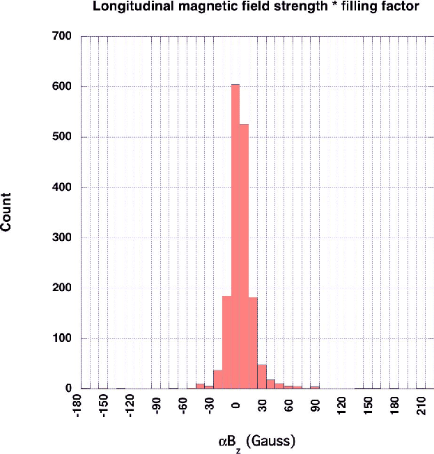
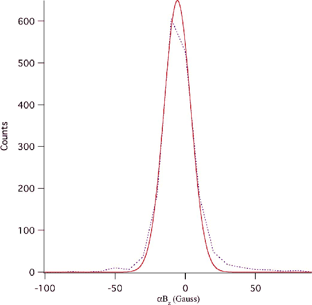
Figure 2:
Histogram of the local average longitudinal magnetic field (the product of the longitudinal magnetic field Bz with the magnetic filling
factor |
| Open with DEXTER | |
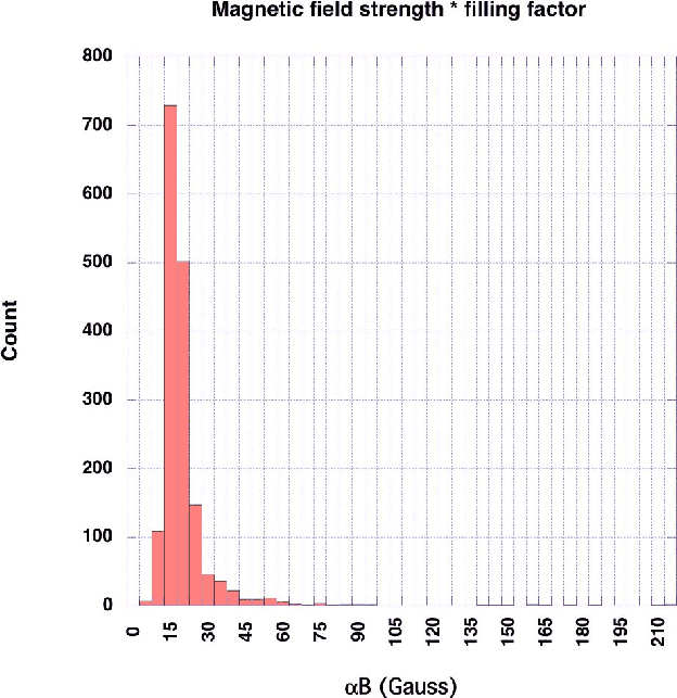
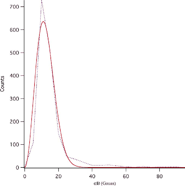
|
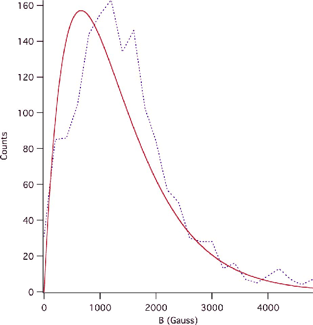
Figure 3:
Histogram of the local average magnetic field strength (the product of the magnetic field strength B with the magnetic filling factor |
| Open with DEXTER | |
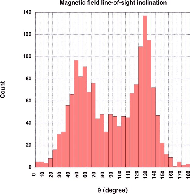
|
Figure 4: Histogram of the magnetic field inclination with respect to the line-of-sight, from the UNNOFIT inversion. The line-of-sight is also the solar vertical with the observation performed at disk center. |
| Open with DEXTER | |
As shown by Bommier et al. (2007), the 2-component inversion of
Fe I 6302.5 Å is unable to separately determine the magnetic filling factor ![]() and the magnetic field strength B, but only their product
and the magnetic field strength B, but only their product ![]() ,
which we call the local average magnetic field
strength. Figures 2-5 display histograms constructed from the
UNNOFIT inversion of the 1680 observed profiles. Figure 2
displays the histogram of the local average longitudinal magnegtic field
,
which we call the local average magnetic field
strength. Figures 2-5 display histograms constructed from the
UNNOFIT inversion of the 1680 observed profiles. Figure 2
displays the histogram of the local average longitudinal magnegtic field
![]() ,
which is the magnetic flux. The unsigned average magnetic
flux is found to be 11 Mx/cm2. Figure 3 displays the
histogram of the local average magnetic field strength
,
which is the magnetic flux. The unsigned average magnetic
flux is found to be 11 Mx/cm2. Figure 3 displays the
histogram of the local average magnetic field strength
![]() for all
the observed profiles. The most probable value is
for all
the observed profiles. The most probable value is
![]() G, the
probability for stronger fields decreasing very fast. The mean value is
G, the
probability for stronger fields decreasing very fast. The mean value is
![]() G and the standard deviation is 14 G.
G and the standard deviation is 14 G.
Figure 4 displays the histogram of the magnetic field vector
inclination. First we recall that an isotropic distribution of field
directions leads to a histogram for the inclination that has a sinusoidal
shape because the elementary surface on the unit sphere is
![]() .
Such a shape was obtained in previous THEMIS observations (Bommier et al. 2007), but it was wrongly concluded that the
magnetic field tends to be horizontal because the inclination angles were
also predominantly ranging between
.
Such a shape was obtained in previous THEMIS observations (Bommier et al. 2007), but it was wrongly concluded that the
magnetic field tends to be horizontal because the inclination angles were
also predominantly ranging between
![]() and
and
![]() .
Disregarding the central hollow, the histogram in Fig. 4
displays the sinusoidal shape expected for the inclination angles of an
isotropic distribution. This central void is the result of the presence of V profiles in all the observed pixels. Simultaneous non-zero Q, U and V is not surprising if many magnetic fields with different inclinations
actually coexist in each resolution element. The central hollow could stem
from our modeling by a single magnetic field per element. Another
explanation for the presence of Stokes V could be some misalignment
problem in the data reduction. We note here that the inclination histogram
of HINODE data by Ishikawa & Tsuneta (2009, see their Fig. 5) also displays a central hollow, although not as
marked as here. From the accuracy test described further, the inclination
angle is determined within
.
Disregarding the central hollow, the histogram in Fig. 4
displays the sinusoidal shape expected for the inclination angles of an
isotropic distribution. This central void is the result of the presence of V profiles in all the observed pixels. Simultaneous non-zero Q, U and V is not surprising if many magnetic fields with different inclinations
actually coexist in each resolution element. The central hollow could stem
from our modeling by a single magnetic field per element. Another
explanation for the presence of Stokes V could be some misalignment
problem in the data reduction. We note here that the inclination histogram
of HINODE data by Ishikawa & Tsuneta (2009, see their Fig. 5) also displays a central hollow, although not as
marked as here. From the accuracy test described further, the inclination
angle is determined within ![]()
![]() .
Considering also the small average number of analyzed profiles per bin
(see the discussion in the next paragraph), it is impossible to ascertain a
departure from the isotropic distribution in the last four bins at the
extremities where the envelope tangent seems to be horizontal, in contrast
to a
.
Considering also the small average number of analyzed profiles per bin
(see the discussion in the next paragraph), it is impossible to ascertain a
departure from the isotropic distribution in the last four bins at the
extremities where the envelope tangent seems to be horizontal, in contrast
to a
![]() envelope.
envelope.
Figure 5 displays the histogram of the azimuth, which is
defined with respect to the slit direction. As the fundamental (
![]() )
ambiguity is not resolved, the azimuth is defined modulo
)
ambiguity is not resolved, the azimuth is defined modulo ![]() between
between
![]() and
and
![]() .
This histogram displays a flat shape on average, also corresponding to
the azimuths of an isotropic distribution. More precisely, the average
number of counts per bin is about
.
This histogram displays a flat shape on average, also corresponding to
the azimuths of an isotropic distribution. More precisely, the average
number of counts per bin is about
![]() .
Assuming a Gaussian noise,
the noise level per bin is
.
Assuming a Gaussian noise,
the noise level per bin is
![]() .
In the figure, the
deviations from bin to bin generally agree with this value, except in some
cases where it is higher. In these cases a positive deviation is, however,
most often immediately followed by a negative one of the same order of
magntitude, and there is no case where this deviation is greater than
.
In the figure, the
deviations from bin to bin generally agree with this value, except in some
cases where it is higher. In these cases a positive deviation is, however,
most often immediately followed by a negative one of the same order of
magntitude, and there is no case where this deviation is greater than
![]() ,
which would be really significant. Thus, we conclude
that in a first approximation our observations indicate an isotropic
distribution of the quiet Sun magnetic field azimuths.
,
which would be really significant. Thus, we conclude
that in a first approximation our observations indicate an isotropic
distribution of the quiet Sun magnetic field azimuths.
We conclude from the THEMIS observations (Bommier et al. 2007) and from these new ZIMPOL observations that the quiet Sun magnetic field has most likely an isotropic distribution of directions. Observations performed at different limb distances by Martínez González et al. (2008b) also conclude on an isotropic distribution of the quiet Sun magnetic field direction. Such observations at different limb distances are indeed needed to thoroughly investigate the field direction distribution. We performed them with ZIMPOL on THEMIS, and we shall discuss them in a future paper of this series. On the basis of our present observations, we do not confirm the horizontal trend of the internetwork magnetic field recently observed by HINODE (Lites et al. 2007,2008) and derived from HINODE inclination histograms by Orozco Suárez et al. (2007b) and Ishikawa & Tsuneta (2009), who could have also been unaware of the sinusoidal shape of the inclination histogram from an isotropical distribution.
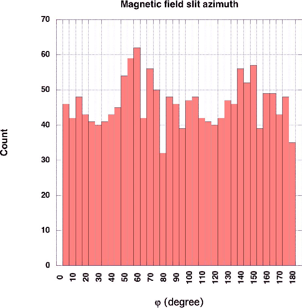
|
Figure 5: Histogram of the magnetic field azimuth with respect to the slit direction, from the UNNOFIT inversion (ambiguity is not resolved). The observation was performed at disk center and the slit was solar north, so that this is also the histogram of the horizontal field component azimuth. |
| Open with DEXTER | |
3.2 Accuracy of the inversion
![\begin{figure}
\par\includegraphics[width=8.5cm,clip]{11373f6a.eps}\par\includegraphics[width=8.5cm,clip]{11373f6b.eps}
\end{figure}](/articles/aa/full_html/2009/42/aa11373-08/img50.png)
|
Figure 6:
Test of the determination of the local average magnetic field strength (the product of the magnetic field strength B with the magnetic filling factor |
| Open with DEXTER | |
|
Figure 7:
Fit of the local average longitudinal magnetic field histogram of Fig. 2 by a Gaussian
|
| Open with DEXTER | |
To determine the accuracy of the magnetic inversion, we performed the same
test as in Bommier et al. (2007), but for the ZIMPOL/THEMIS polarimetric
accuracy (
![]() in the continuum under the conditions described
in Sect. 2)
and spectral sampling. As in that paper,
a series of theoretical profiles was generated from the Unno-Rachkovsky
solution applied to the 2-component atmosphere, for a set of magnetic
field
strength, inclination, azimuth, and filling factor values. These
profiles
were then noised at the observed level and submitted to the UNNOFIT
inversion. The test consists in comparing the output values with the
known
input ones. The main result is presented in Fig. 6, which is
analogous to Fig. 4 of Bommier et al. (2007), and it shows analogously
that the local average magnetic field strength
in the continuum under the conditions described
in Sect. 2)
and spectral sampling. As in that paper,
a series of theoretical profiles was generated from the Unno-Rachkovsky
solution applied to the 2-component atmosphere, for a set of magnetic
field
strength, inclination, azimuth, and filling factor values. These
profiles
were then noised at the observed level and submitted to the UNNOFIT
inversion. The test consists in comparing the output values with the
known
input ones. The main result is presented in Fig. 6, which is
analogous to Fig. 4 of Bommier et al. (2007), and it shows analogously
that the local average magnetic field strength ![]() (the product of
the field strength by the filling factor) is correctly determined by the
inversion. The bottom figure is a zoom of the top figure near the axis
origin, and shows the dispersion of the results about the first diagonal
that represents equal input and output. This dispersion is on the order of
10 G, which we retain as the accuracy on the local average magnetic field
strength determination. This dispersion includes both longitudinal and
transverse fields. Moreover, the bottom figure shows that, when the input
local average magnetic field strength decreases to zero, the output
saturates at 10 G. In Fig. 4 of Bommier et al. (2007), the saturation
level is 25 G for a polarimetric accuracy of only
(the product of
the field strength by the filling factor) is correctly determined by the
inversion. The bottom figure is a zoom of the top figure near the axis
origin, and shows the dispersion of the results about the first diagonal
that represents equal input and output. This dispersion is on the order of
10 G, which we retain as the accuracy on the local average magnetic field
strength determination. This dispersion includes both longitudinal and
transverse fields. Moreover, the bottom figure shows that, when the input
local average magnetic field strength decreases to zero, the output
saturates at 10 G. In Fig. 4 of Bommier et al. (2007), the saturation
level is 25 G for a polarimetric accuracy of only
![]() .
It
thus appears that the saturation level is directly related to the
polarimetric accuracy. The regular pattern detectable in the lower part of
Fig. 6 is a consequence of the regular spacing of the input
theoretical data. The number of input points is 183 600 and the number of
output points that depart from more than about 10 G from the diagonal is
about 5% of the total number of points.
.
It
thus appears that the saturation level is directly related to the
polarimetric accuracy. The regular pattern detectable in the lower part of
Fig. 6 is a consequence of the regular spacing of the input
theoretical data. The number of input points is 183 600 and the number of
output points that depart from more than about 10 G from the diagonal is
about 5% of the total number of points.
The observed profile asymmetries, which are visible in Fig. 1, are taken into account neither in the test nor in the inversion. Such asymmetries may be due to vertical gradient of the radial velocity. A new version of our inversion code UNNOFIT is under development, which takes into account such gradients and is able to properly fit asymmetric profiles. At first sight the magnetic field strength would not be highly modified. Besides, it may be noted that the asymmetries' order of magnitude is comparable to the polarimetric noise in Fig. 1, at least in Q/I and U/I.
Figures 7 and 8 display Gaussian
fits of the histograms of Figs. 2 and 3,
corresponding respectively to the local average longitudinal magnetic field
and to the local average magnetic field strength. The histogram of Fig. 2 can be fitted with the usual Gaussian
![]() .
The histogram in Fig. 3 can be fitted
by the Maxwell distribution
.
The histogram in Fig. 3 can be fitted
by the Maxwell distribution
![]() .
These fits show
that the magnetic field vector has a Gaussian distribution, since a Gaussian
distribution leads to a Maxwell distribution after angle averaging. The
width w of the Gaussian and Maxwellian are 13.5 G and 11 G, respectively.
Since these values are not significantly higher than the 10 G corresponding
to the inversion accuracy, we cannot conclude that the local average
magnetic field truly has a Gaussian PDF, so we attribute the Gaussian shape
of these histogram envelopes to the polarimetric noise.
.
These fits show
that the magnetic field vector has a Gaussian distribution, since a Gaussian
distribution leads to a Maxwell distribution after angle averaging. The
width w of the Gaussian and Maxwellian are 13.5 G and 11 G, respectively.
Since these values are not significantly higher than the 10 G corresponding
to the inversion accuracy, we cannot conclude that the local average
magnetic field truly has a Gaussian PDF, so we attribute the Gaussian shape
of these histogram envelopes to the polarimetric noise.
|
Figure 8:
Fit of the local average magnetic field strength histogram of Fig. 3 by a Maxwellian
|
| Open with DEXTER | |
4 Second step: direct determination of the magnetic filling factor
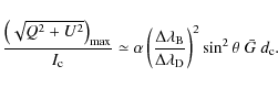
From the weak field laws, which express the emerging polarization Stokes
parameters in terms of the derivatives of the intensity profile,
Landi Degl'Innocenti & Landolfi (2004, pp. 405-407) derive the approximate expressions
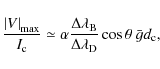
We have introduced here the magnetic filling factor

|
(3) |
where
|
(4) |
where

|
(5) |
where
We now note that the linear polarization depends quadratically on the
magnetic field strength and direction, but linearly on the magnetic filling
factor. Taking the square of Eq. (1) and dividing by Eq. (2), we find
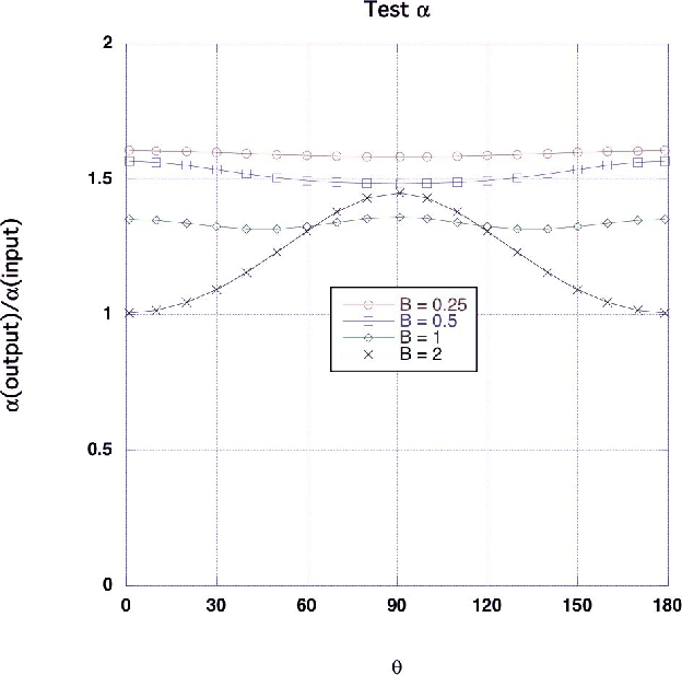
Figure 9 displays a test of this approximation. The Stokes parameters are first computed with the Unno-Rachkovsky solution applied to a 2-component atmosphere with a given value of
|
Figure 9:
Test of the determination of the magnetic filling factor by applying Eq. (6)
to the polarimetric data. For the test, the polarimetric data were
theoretical profiles computed from the Unno-Rachkovsky solution,
weighted by a theoretical input magnetic filling factor |
| Open with DEXTER | |
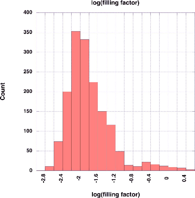
|
Figure 10: Histogram of the filling factor, determined from the polarization data complemented by the UNNOFIT inversion results on the field inclination (see Eq. (6)). The abscissa is in logarithmic scale. |
| Open with DEXTER | |
In Fig. 10, we plotted the histogram derived from the
application of Eq. (6) to our data. The inclination angle value ![]() was taken from the UNNOFIT inversion results. We thus obtain a
filling factor
was taken from the UNNOFIT inversion results. We thus obtain a
filling factor ![]() ranging between
ranging between
![]() and
and
![]() ,
with a maximum probability at
,
with a maximum probability at
![]() .
The mean value is
.
The mean value is
![]() .
The standard deviation of
.
The standard deviation of
![]() is 0.5. The values
higher than unity have no physical meaning and come from the fact that for a
quasi-horizontal field, when
is 0.5. The values
higher than unity have no physical meaning and come from the fact that for a
quasi-horizontal field, when ![]() is close to
is close to
![]() ,
,
![]() becomes very large.
becomes very large.
From the polarimetric accuracy
![]() of our
ZIMPOL/THEMIS data (S being any of the Stokes parameters I,Q,U,V), we
find that the relative error predicted by Eq. (6) is
of our
ZIMPOL/THEMIS data (S being any of the Stokes parameters I,Q,U,V), we
find that the relative error predicted by Eq. (6) is
|
(7) |
Because
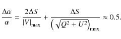
5 The magnetic field probability density function
|
Figure 11:
Histogram of the magnetic field strength, derived by dividing the local average magnetic field strength |
| Open with DEXTER | |
|
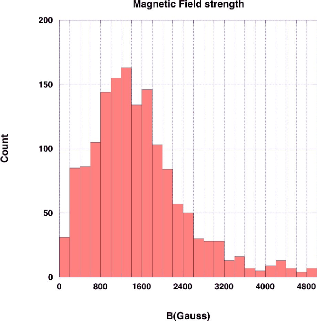
Figure 12:
Behavior of the magnetic filling factor |
| Open with DEXTER | |
|
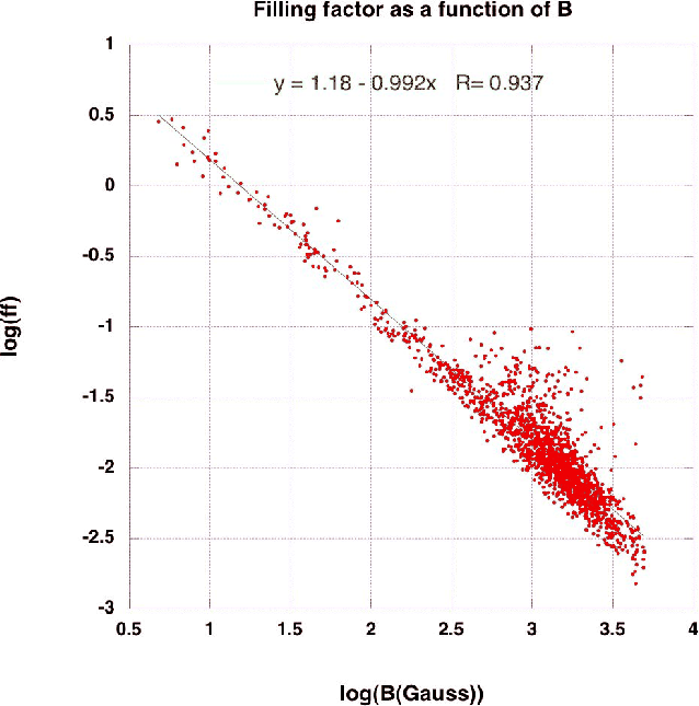
Figure 13:
2D histogram of the magnetic filling factor and of the magnetic field strength B, each pair of them known in each solar pixel. This figure is a 3D representation of the number of points in Fig. 12. The joint PDF
|
| Open with DEXTER | |
For each of the 1680 observed solar pixels (determined by the slit width and
the camera pixel size along the slit), the local average magnetic field
strength ![]() was obtained from the UNNOFIT inversion (Sect. 3), and the magnetic filling factor
was obtained from the UNNOFIT inversion (Sect. 3), and the magnetic filling factor ![]() was
directly and independently determined from the spectropolarimetric data
(Sect. 4). The magnetic field strength value is
then obtained by performing the ratio
was
directly and independently determined from the spectropolarimetric data
(Sect. 4). The magnetic field strength value is
then obtained by performing the ratio
![]() for each pixel, and
the magnetic field strength B histogram follows (Fig. 11). The
PDF of the magnetic field strength is then the envelope of this histogram.
The tail of very strong fields that appears in the histogram stems from the
noise contribution, but detecting strong fields associated to small filling
factors is not new
(see for instance Socas-Navarro & Sánchez Almeida 2002; Domínguez Cerdeña et al. 2003b,a; Grossmann-Doerth et al. 1996).
Khomenko et al. (2003) obtained a B histogram similar in shape to ours,
but with lower field strengths. Their histogram is devoid of any filling
factor effect, because it results from direct Zeeman splitting measurement
in IR profiles, where the Zeeman effect is stronger. However, as clearly
shown by their Figs. 2 and 4, the Zeeman components are not yet completely
resolved (in the near IR range), so that the real situation is probably
inbetween the weak field approximation described by our Eq. (1)
where the component separation does not depend on the field strength but
instead on the derivative of the intensity profile and the completely
resolved Zeeman effect. This circumstance could explain the lowest field
strengths reported by these authors.
for each pixel, and
the magnetic field strength B histogram follows (Fig. 11). The
PDF of the magnetic field strength is then the envelope of this histogram.
The tail of very strong fields that appears in the histogram stems from the
noise contribution, but detecting strong fields associated to small filling
factors is not new
(see for instance Socas-Navarro & Sánchez Almeida 2002; Domínguez Cerdeña et al. 2003b,a; Grossmann-Doerth et al. 1996).
Khomenko et al. (2003) obtained a B histogram similar in shape to ours,
but with lower field strengths. Their histogram is devoid of any filling
factor effect, because it results from direct Zeeman splitting measurement
in IR profiles, where the Zeeman effect is stronger. However, as clearly
shown by their Figs. 2 and 4, the Zeeman components are not yet completely
resolved (in the near IR range), so that the real situation is probably
inbetween the weak field approximation described by our Eq. (1)
where the component separation does not depend on the field strength but
instead on the derivative of the intensity profile and the completely
resolved Zeeman effect. This circumstance could explain the lowest field
strengths reported by these authors.
Thus, for each pixel, we find one ![]() and one B value. These
values can be used to place a point representing the pixel in the
and one B value. These
values can be used to place a point representing the pixel in the
![]() -
-![]() axes, thus giving a scatter plot where all the 1680 pixels are represented (Fig. 12). We find that these data are
well-fitted (in the log-log coordinates) by the linear function
axes, thus giving a scatter plot where all the 1680 pixels are represented (Fig. 12). We find that these data are
well-fitted (in the log-log coordinates) by the linear function
| (8) |
which is

with B1=15 G. The form of this very simple relation partly comes from the
A 2D histogram can be built from Fig. 12 by defining 2D bins and
counting the number of points falling inside each 2D bin. This histogram is
represented in Fig. 13. Its envelope is the joint PDF of the two
random variables ![]() and B, that we denote as
and B, that we denote as
![]() .
The
shape of the envelope (and Fig. 12) shows that these two variables
are strongly correlated. The magnetic field PDF (the envelope of the
histogram of Fig. 11) is the marginal PDF
.
The
shape of the envelope (and Fig. 12) shows that these two variables
are strongly correlated. The magnetic field PDF (the envelope of the
histogram of Fig. 11) is the marginal PDF
|
(10) |
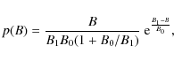
Similarly, the envelope of Fig. 10 is the other marginal PDF,
For the benefit of the reader, we give the definition of the joint PDF of two random variables in Appendix A, and the related marginal PDFs (see also Papoulis 1965, Chap. 6).
5.1 Discussion of the magnetic field PDF
|
Figure 14:
Weighted histogram of the magnetic field strength. For each bin of the magnetic field strength histogram of Fig. 11, the count number has been multiplied by the average magnetic field filling factor for this magnetic field strength
|
| Open with DEXTER | |
Confusion is encountered in the literature about the definition of the
magnetic field PDF. This comes from the quiet Sun magnetic field being a
complex quantity, having a PDF for both its field strength and magnetic
filling factor, at least in data interpretation where these two quantities
are determined in each pixel, the magnetic filling factor ![]() representing the fraction of the resolution element covered by the magnetic
field B. From the modeling point of view, the necessity of introducing the
magnetic filling factor
representing the fraction of the resolution element covered by the magnetic
field B. From the modeling point of view, the necessity of introducing the
magnetic filling factor ![]() is less evident, and one has to carefully
examine the modeling conditions, i.e. with or without filling factor, before
comparing the magnetic field PDFs. Thus, the following discussion will be
divided into several parts corresponding to different approaches.
is less evident, and one has to carefully
examine the modeling conditions, i.e. with or without filling factor, before
comparing the magnetic field PDFs. Thus, the following discussion will be
divided into several parts corresponding to different approaches.
5.1.1 Comparison with Sánchez Almeida's definition
For the interpretation of observations concerning the solar internetwork,
Sánchez Almeida et al. (2003) introduce a quantity referred to as
magnetic field PDF and defined as being
proportional to the sum of filling factors of all those
measurements (i.e. of field strength B) in the bin
![]() . In Sánchez Almeida (2007), this definition is rephrased
as the fraction of quiet Sun occupied by magnetic field of
each strength. The same definition is used in
Domínguez Cerdeña et al. (2006b,a). An explicit definition of
this quantity is given in Eq. (14) of Martínez González et al. (2008a). Starting
from this equation, we find that this so-called PDF can be written as
. In Sánchez Almeida (2007), this definition is rephrased
as the fraction of quiet Sun occupied by magnetic field of
each strength. The same definition is used in
Domínguez Cerdeña et al. (2006b,a). An explicit definition of
this quantity is given in Eq. (14) of Martínez González et al. (2008a). Starting
from this equation, we find that this so-called PDF can be written as
![]() ,
with p(B) the magnetic field marginal PDF introduced
above and
,
with p(B) the magnetic field marginal PDF introduced
above and
|
(11) |
Here,
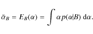
Martínez González et al. (2008a) rightly mention that their PDF takes into account the filling factor. We think that it is not a good idea to call the product
We now explain why this quantity
![]() is very useful for
solar polarization modeling, although it is not a true magnetic field PDF.
For this purpose, let us recall that the first Stokes parameter I is the
specific intensity of radiation in erg/cm2/s/sr/Hz. This means that the
energy
is very useful for
solar polarization modeling, although it is not a true magnetic field PDF.
For this purpose, let us recall that the first Stokes parameter I is the
specific intensity of radiation in erg/cm2/s/sr/Hz. This means that the
energy ![]() emitted by the elementary surface
emitted by the elementary surface ![]() during
the elementary time interval
during
the elementary time interval ![]() in the elementary solid angle
in the elementary solid angle
![]() and frequency interval
and frequency interval
![]() is
is
| (13) |
The other Stokes parameters Q,U,V have the same unit. For this reason, when computing, say, the average emitted
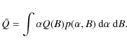
|
(14) |
For simplicity we assume that Stokes Q only depends on the magnetic field strength. Using Eq. (12), we obtain
which demonstrates the exact physical meaning of the quantity
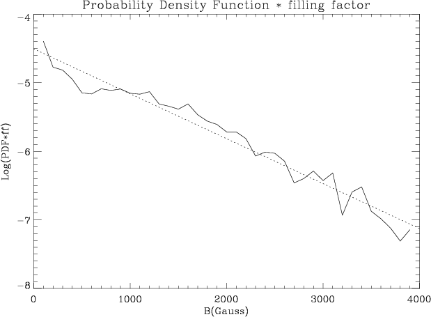
5.1.2 Analytical fit giving the magnetic field PDF
In Fig. 14 we have plotted the histogram that has
![]() as envelope, for comparison with Fig. 6 (right) of
Martínez González et al. (2008a) and with Fig. 3 of Sánchez Almeida et al. (2003)
(although this last figure concerns longitudinal magnetic fields). It can be
seen that the agreement with the IR data recommended by
Martínez González et al. (2008a) is fairly good, although our field strengths are
a bit higher. We agree with Martínez González et al. (2008a) on the linear
behavior of the histogram (in log-lin coordinates). The linear fit of our
data is
as envelope, for comparison with Fig. 6 (right) of
Martínez González et al. (2008a) and with Fig. 3 of Sánchez Almeida et al. (2003)
(although this last figure concerns longitudinal magnetic fields). It can be
seen that the agreement with the IR data recommended by
Martínez González et al. (2008a) is fairly good, although our field strengths are
a bit higher. We agree with Martínez González et al. (2008a) on the linear
behavior of the histogram (in log-lin coordinates). The linear fit of our
data is
where A is a constant to be determined by normalization, and B0=660 G. Assuming that
|
(17) |
so that finally
with B1=15 G, B0=660 G, and
|
Figure 15: Fit of magnetic field strength histogram of Fig. 11 by the magnetic field PDF p(B) derived from the linear fits of Figs. 12 and 14. This magnetic field PDF is given by Eq. (18). |
| Open with DEXTER | |
5.1.3 Comparison with volume-filling PDFs
Let us call volume-filling PDF, the
PDF of a magnetic field present everywhere in the medium. In this case ![]() and the PDFs proposed in the literature have to be compared with
the envelope of our local average magnetic field
and the PDFs proposed in the literature have to be compared with
the envelope of our local average magnetic field ![]() histograms. One
also has to carefully examine whether the proposed PDF concerns the
absolute field strength or the longitudinal field that is one component only
of the field vector. We note that the consideration of the volume-filling
longitudinal field is quite relevant, because this is the magnetic flux. We
also note that in the case of a volume-filling magnetic field, the magnetic
field PDF p(B) is indeed the fraction of the solar surface occupied by
fields with values between B and
histograms. One
also has to carefully examine whether the proposed PDF concerns the
absolute field strength or the longitudinal field that is one component only
of the field vector. We note that the consideration of the volume-filling
longitudinal field is quite relevant, because this is the magnetic flux. We
also note that in the case of a volume-filling magnetic field, the magnetic
field PDF p(B) is indeed the fraction of the solar surface occupied by
fields with values between B and
![]() (see the detailed discussion in
Appendix A).
(see the detailed discussion in
Appendix A).
In this category, one finds the determination of the magnetic flux PDF by Stenflo & Holzreuter (2003). As the flux distribution is derived from magnetograms, it has to be compared with our Figs. 2 and 7. The widths of the distributions (13.5 G ours, 17.0 G theirs) are comparable and in good agreement with the polarimetric accuracy of the corresponding measurements. The authors consider the wings of the distribution in detail. Probably, the wings are caused by network pixels that bear a stronger field and are visible in their magnetograms (Fig. 1). Such pixels cannot be avoided in the measurements. Our distribution also has broader wings than Gaussian, visible in logarithmic scale in Fig. 16, but we have a much lower pixel number in our analysis. In the same category one finds the theoretical study by Berrilli et al. (2008). This is also a longitudinal flux PDF to be compared with our Figs. 2 and 7. As is visible in Fig. 16, we do not have enough pixels to validate or invalidate this model with our observations.
We now turn to the field strength distribution. Inspired by the exponential
PDF obtained by Martínez González et al. (2008a), Trujillo Bueno et al. (2004)
introduced an exponential distribution for the volume-filling field
strength,
![]() ,
to fit a series of Hanle effect
measurements of the turbulent quiet Sun magnetic field. In addition, the
field is assumed to be microturbulent with an isotropic angular
distribution. With B0=130 G, the fit is rather satisfactory. It should
also be mentioned that the same data can be fitted almost equally well with
a single-valued magnetic field (PDF in the form of a Dirac distribution)
with a strength of B=60 G. Our B0 value of 660 G differs notably,
however, from this 130 G value, because they assume
,
to fit a series of Hanle effect
measurements of the turbulent quiet Sun magnetic field. In addition, the
field is assumed to be microturbulent with an isotropic angular
distribution. With B0=130 G, the fit is rather satisfactory. It should
also be mentioned that the same data can be fitted almost equally well with
a single-valued magnetic field (PDF in the form of a Dirac distribution)
with a strength of B=60 G. Our B0 value of 660 G differs notably,
however, from this 130 G value, because they assume ![]() (volume-filling magnetic field) in their simulation. This may also be due to
the shape of our PDF that decreases towards zero at the axis origin, as well
as our
(volume-filling magnetic field) in their simulation. This may also be due to
the shape of our PDF that decreases towards zero at the axis origin, as well
as our ![]() histogram in Figs. 3 and 8, as does the Maxwellian distribution function, whereas their
theoretical distribution does not. Considering our result of
histogram in Figs. 3 and 8, as does the Maxwellian distribution function, whereas their
theoretical distribution does not. Considering our result of
![]() with B1=15 G, the filling factor remains close to unity for
weak fields as those detected by Hanle effect interpretation, so that their
hypothesis of volume-filling may be found coherent with our results for weak
fields. As mentioned in our conclusion, the derived PDF may depend on the
sensitivity of the magnetic field measurement method (Hanle effect is
sensitive to weak and unresolved fields, Zeeman effect is sensitive to the
strongest fields). The mean value B=60 G that they derive under the
hypothesis of volume-filling and single-valued microturbulent field remains
comparable to our mean value
with B1=15 G, the filling factor remains close to unity for
weak fields as those detected by Hanle effect interpretation, so that their
hypothesis of volume-filling may be found coherent with our results for weak
fields. As mentioned in our conclusion, the derived PDF may depend on the
sensitivity of the magnetic field measurement method (Hanle effect is
sensitive to weak and unresolved fields, Zeeman effect is sensitive to the
strongest fields). The mean value B=60 G that they derive under the
hypothesis of volume-filling and single-valued microturbulent field remains
comparable to our mean value
![]() G.
G.
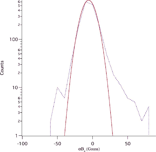
|
Figure 16: Same as Fig. 7, but with the number of pixels per bin (counts) plotted on a logarithmic scale to highlight the distribution in the wings. |
| Open with DEXTER | |
5.1.4 Comparison with HINODE results
We now discuss the results by Orozco Suárez et al. (2007b) and
Ishikawa & Tsuneta (2009). Both papers show a magnetic field strength PDF
with a maximum in the hG range. A careful examination shows that their PDF
definition is correct and is the same as ours, and that the differences in
the results (our PDF peaks at higher field strengths) have to be assigned to
a difference in the measurement of the magnetic filling factor. All these
studies apply a Milne-Eddington inversion to the spectropolarimeteric data,
with filling factor. As mentioned in Bommier et al. (2007), only the local
average magnetic field strength ![]() can be retrieved from this
inversion. It can be verified that both works agree when looking at this
product
can be retrieved from this
inversion. It can be verified that both works agree when looking at this
product ![]() :
their field strengths are lower than ours, but their
filling factor are higher than ours, so that the order of magnitude of their
product is the same. We emphasize that their filling factor
:
their field strengths are lower than ours, but their
filling factor are higher than ours, so that the order of magnitude of their
product is the same. We emphasize that their filling factor ![]() is
defined by the rate of stray light, which is also assumed to be the
proportion of light coming from the unmagnetic region (note that their
is
defined by the rate of stray light, which is also assumed to be the
proportion of light coming from the unmagnetic region (note that their ![]() corresponds to our
corresponds to our ![]() )
)
The question lies in the filling factor method of measurement. Ours is described above and is performed independently of the Milne-Eddington inversion. They derive the filling factor by comparing, in a first step, local intensity profiles (no polarization at that step) with average intensity profiles assumed to represent the zero field situation. This is the method introduced by Skumanich & Lites (1987) and discussed by Lites & Skumanich (1990). Depending of the activity level of the map under study, this average profile is evaluated either by a global average or by a local average on the less active part on the map. In the present case of quiet Sun studies, this profile is determined by a local average evaluated around the pixel of interest. Considering that this approach gives a different result from ours, we are led to raise the question to know whether such a method really determines the nonmagnetic profile. If this average profile is taken from the whole map (global average) or from a less active but wide part of it, we note that the local physical parameters at the pixel under study (temperature, density) may not be fully taken into account in the nonmagnetic global profile. And if this average is performed on the neighbor pixels only as in the above-mentioned studies, we raise the question: is the local average really nonmagnetic with respect to the considered pixel?
5.1.5 What can be expected from Fe I 6302.5 measurements?
When the quiet Sun magnetic field strength B is discussed, this magnetic
field also has a magnetic filling factor ![]() .
The question is how to
determine
.
The question is how to
determine ![]() and B separately. As discussed in
Bommier et al. (2007), it is not possible to determine
and B separately. As discussed in
Bommier et al. (2007), it is not possible to determine ![]() and Bseparately from inversion of Fe I 6302.5 Å data, but only their
product
and Bseparately from inversion of Fe I 6302.5 Å data, but only their
product ![]() .
This is because, for solar magnetic field strengths and
for a visible line like Fe I 6302.5 Å, the Zeeman splitting unit
.
This is because, for solar magnetic field strengths and
for a visible line like Fe I 6302.5 Å, the Zeeman splitting unit
![]() remains smaller or close to the Doppler width
remains smaller or close to the Doppler width
![]() .
This behavior can be expected for any line in
the visible range. On the contrary, when the Zeeman components are
separated, determining
.
This behavior can be expected for any line in
the visible range. On the contrary, when the Zeeman components are
separated, determining ![]() and B separately, by inversion, becomes
possible. This is partly true at infrared wavelengths (see the discussion at
the beginning of Sect. 5). That is why
Martínez González et al. (2008a) are able to get reliable results by inverting
infrared lines, and we get results in agreement with theirs by applying our
direct
and B separately, by inversion, becomes
possible. This is partly true at infrared wavelengths (see the discussion at
the beginning of Sect. 5). That is why
Martínez González et al. (2008a) are able to get reliable results by inverting
infrared lines, and we get results in agreement with theirs by applying our
direct ![]() determination complementing the inversion of the visible
Fe I 6302.5 Å line. Examining the work of
Martínez González et al. (2008a), it can be seen that they are not confident in
the Fe I 6302.5 Å results in separate
determination complementing the inversion of the visible
Fe I 6302.5 Å line. Examining the work of
Martínez González et al. (2008a), it can be seen that they are not confident in
the Fe I 6302.5 Å results in separate ![]() and B, because
they find that these results depend on the initialization of the inversion;
however, it can be seen in their paper that the magnetic flux, which is the
longitudinal counterpart of the product
and B, because
they find that these results depend on the initialization of the inversion;
however, it can be seen in their paper that the magnetic flux, which is the
longitudinal counterpart of the product ![]() ,
remains unchanged
whatever the initialization be. This confirms that the inversion of visible
Fe I 6302.5 Å data accurately recovers the local average magnetic
field strength
,
remains unchanged
whatever the initialization be. This confirms that the inversion of visible
Fe I 6302.5 Å data accurately recovers the local average magnetic
field strength ![]() ,
though it is not able to recover
,
though it is not able to recover ![]() and Bseparately.
and Bseparately.
6 Conclusions
We find that the magnetic field filling factor ![]() is related to the
magnetic field strength B by the simple approximate law
is related to the
magnetic field strength B by the simple approximate law
![]() with B1=15 G. Moreover, we find that the magnetic field PDF can be
expressed by the analytical law of Eq. (18). This means that the
medium is complex and various field strengths may be encountered: (i) the
1500 Gauss field filling 1% of space as seen in the tails of the magnetic
field distributions by Khomenko et al. (2003), Martínez González et al. (2006),
Orozco Suárez et al. (2007b), Martínez González et al. (2008a), as also detected by
Domínguez Cerdeña et al. (2003b,2006b,2003a,2006a)
; (ii) the 150 Gauss field filling 10% of space as seen from incomplete
Paschen-Back effect interpretation by López Ariste et al. (2007) and
Sánchez Almeida et al. (2008); (iii) 20-50 Gauss field filling the major part of
space, as seen from the Hanle effect interpretation (see the measurement
review by Trujillo Bueno et al. (2004) and Trujillo Bueno et al. (2006) for the Sr
I 4607 line, see also Bommier et al. (2006) for a series of MgH lines).
with B1=15 G. Moreover, we find that the magnetic field PDF can be
expressed by the analytical law of Eq. (18). This means that the
medium is complex and various field strengths may be encountered: (i) the
1500 Gauss field filling 1% of space as seen in the tails of the magnetic
field distributions by Khomenko et al. (2003), Martínez González et al. (2006),
Orozco Suárez et al. (2007b), Martínez González et al. (2008a), as also detected by
Domínguez Cerdeña et al. (2003b,2006b,2003a,2006a)
; (ii) the 150 Gauss field filling 10% of space as seen from incomplete
Paschen-Back effect interpretation by López Ariste et al. (2007) and
Sánchez Almeida et al. (2008); (iii) 20-50 Gauss field filling the major part of
space, as seen from the Hanle effect interpretation (see the measurement
review by Trujillo Bueno et al. (2004) and Trujillo Bueno et al. (2006) for the Sr
I 4607 line, see also Bommier et al. (2006) for a series of MgH lines).
Because the kG internetwork field with very small filling factors were previously detected (Sánchez Almeida & Lites 2000; Grossmann-Doerth et al. 1996), recent magnetoconvection modeling (Bushby et al. 2008) shows that fields stronger than the equipartition value could result from localized concentrations due to convective intergranular downflows. However, it should be noted that our results have to be taken with care because our field determination is based on a 2-component inversion, whereas we arrive at the vision of a complex medium where all the field strengths coexist.
Actually, each magnetic field determination (Zeeman, hyperfine structure,
Hanle) has its own sensitivity domain. Because it is a linear effect, the
Zeeman effect detects the stronger fields better even if they do not fill
the whole space. In contrast, the Hanle effect, being highly nonlinear,
cannot detect the strong fields. To prove this point, let us assume a
2-component atmosphere with a 2000 Gauss field filling 2% of space: 98%
of the scattered radiation will not be depolarized, while 2% will only be
depolarized by the Hanle effect. As a 2000 G field corresponds to the
saturation regime of the Hanle effect, the corresponding linear polarization
is 1/5 of the zero field one. As a result, the global polarization
remains almost insensitive to strong intermittent magnetic fields. In
contrast, the Hanle effect is sensitive to weak field filling the major part
of space. The incomplete Paschen-Back effect is sensitive to hG fields, but
also is unable to detect kG fields. The result of our paper is that the
strong, intermediate, and weak fields cohabit, with different filling
factors obeying the simple approximate law
![]() with B1=15 G.
with B1=15 G.
In a later paper of this series, we will analyze the center-to-limb variation of the quiet Sun polarization with ZIMPOL on THEMIS observations, in order to thoroughly investigate the field direction distribution function. Further observations with a better polarimetric accuracy are, however, needed to confirm the results obtained in the present work.
AcknowledgementsThe authors are grateful and indebted to D. Gisler and A. Feller for having provided the ZIMPOL data reduction package adapted to THEMIS, and to the whole ZIMPOL and THEMIS teams and to J.O. Stenflo for having given them the possibility of using ZIMPOL on THEMIS. They are also grateful to the anonymous referee for the kind and very helpful comments. Thanks also to J. Adams for the excellent english language corrections. The ZIMPOL campaign at THEMIS was financed by the SNF grant 200020-117821. A.A.R. acknowledges financial support by the Spanish Ministry of Education and Science through project AYA2007-63881.
References
- Berrilli, F., Del Moro, D., & Viticchiè, B. 2008, A&A, 489, 763 [NASA ADS] [CrossRef] [EDP Sciences]
- Bommier, V., Landi Degl'Innocenti, E., Feautrier, N., & Molodij, G. 2006, A&A, 458, 625 [NASA ADS] [CrossRef] [EDP Sciences]
- Bommier, V., Landi Degl'Innocenti, E., Landolfi, M., & Molodij, G. 2007, A&A, 464, 323 [NASA ADS] [CrossRef] [EDP Sciences]
- Bushby, P. J., Houghton, S. M., Proctor, M. R. E., & Weiss, N. O. 2008, MNRAS, 387, 698 [NASA ADS] [CrossRef]
- Domínguez Cerdeña, I., Sánchez Almeida, J., & Kneer, F. 2003a, A&A, 407, 741 [NASA ADS] [CrossRef] [EDP Sciences]
- Domínguez Cerdeña, I., Kneer, F., & Sánchez Almeida, J. 2003b, ApJ, 582, L55 [NASA ADS] [CrossRef]
- Domínguez Cerdeña, I., Sánchez Almeida, J., & Kneer, F. 2006a ApJ, 636, 496
- Domínguez Cerdeña, I., Almeida, J. S., & Kneer, F. 2006b, ApJ, 646, 1421 [NASA ADS] [CrossRef]
- Faurobert-Scholl, M. 1992, A&A, 258, 521 [NASA ADS]
- Gandorfer, A. M., & Povel, H. P. 1997, A&A, 328, 381 [NASA ADS]
- Gandorfer, A. M., Steiner, H. P. P. P., Aebersold, F., et al. 2004, A&A, 422, 703 [NASA ADS] [CrossRef] [EDP Sciences]
- Grossmann-Doerth, U., Keller, C. U., & Schuessler, M. 1996, A&A, 315, 610 [NASA ADS]
- Ishikawa, R., & Tsuneta, S. 2009, A&A, 495, 607 [NASA ADS] [CrossRef] [EDP Sciences]
- Khomenko, E. V., & Collados, M. 2007, ApJ, 659, 1726 [NASA ADS] [CrossRef]
- Khomenko, E. V., Collados, M., Solanki, S. K., Lagg, A., & Trujillo Bueno, J. 2003, A&A, 408, 1115 [NASA ADS] [CrossRef] [EDP Sciences]
- Landolfi, M., Landi Degl'Innocenti, E., & Arena, P. 1984, Sol. Phys., 93, 269 [NASA ADS] [CrossRef]
- Landi Degl'Innocenti, E. 1976, A&AS, 25, 379 [NASA ADS]
- Landi Degl'Innocenti, E., & Landolfi, M. 2004, Polarization in Spectral Lines (Dordrecht: Kluwer Academ. Publ.)
- Lites, B., Socas-Navarro, H., Kubo, M., et al. 2007, PASJ, 59, 571
- Lites, B. W., & Skumanich, A. 1990, ApJ, 348, 747 [NASA ADS] [CrossRef]
- Lites, B. W., & Socas-Navarro, H. 2004, ApJ, 613, 600 [NASA ADS] [CrossRef]
- Lites, B. W., Kubo, M., Socas-Navarro, H., et al. 2008, ApJ, 672, 1237 [NASA ADS] [CrossRef]
- López Ariste, A., Tomczyk, S., & Casini, R. 2006, A&A, 454, 663 [NASA ADS] [CrossRef] [EDP Sciences]
- López Ariste, A., Martínez González, M. J., & Ramírez Vélez, J. C. 2007, A&A, 464, 351 [NASA ADS] [CrossRef] [EDP Sciences]
- Maltby, P., Avrett, E. H., Carlsson, M., et al. 1986, ApJ, 306, 284 [NASA ADS] [CrossRef]
- Martínez González, M. J., Collados, M., & Ruiz Cobo, B. 2006, A&A, 456, 1159 [NASA ADS] [CrossRef] [EDP Sciences]
- Martínez González, M. J., Collados, M., Ruiz Cobo, B., & Beck, C. 2008a, A&A, 477, 953 [NASA ADS] [CrossRef] [EDP Sciences]
- Martínez González, M. J., Asensio Ramos, A., López Ariste, A., & Manso Sainz, R. 2008b, A&A, 479, 229 [NASA ADS] [CrossRef] [EDP Sciences]
- Orozco Suárez, D., Bellot Rubio, L., & del Toro Iniesta, J. C. 2007a, ApJ, 662, 31 [NASA ADS] [CrossRef]
- Orozco Suárez, D., Bellot Rubio, L., del Toro Iniesta, J. C., et al. 2007b, ApJ, 670, L61 [NASA ADS] [CrossRef]
- Papoulis, A. 1965, in Probability, Random Variables and Stochastic Processes (New-York: Mc Graw-Hill)
- Ramírez Vélez, J. C., López Ariste, A., & Semel, M. 2008, A&A, 487, 731 [NASA ADS] [CrossRef] [EDP Sciences]
- Sánchez Almeida, J. 2007, ApJ, 657, 1150 [NASA ADS] [CrossRef]
- Sánchez Almeida, J., & Lites, B. W. 2000, ApJ, 532, 1215 [NASA ADS] [CrossRef]
- Sánchez Almeida, J., Domínguez Cerdeña, I., & Kneer, F. 2003, ApJ, 597, L177 [NASA ADS] [CrossRef]
- Sánchez Almeida, J., Viticchié, B., Landi Degl'Innocenti, E., & Berrilli, F. 2008, ApJ, 675, 906 [NASA ADS] [CrossRef]
- Skumanich, A., & Lites, B. W. 1987, ApJ, 322, 473 [NASA ADS] [CrossRef]
- Socas-Navarro, H., & Sánchez Almeida, J. 2002, ApJ, 565, 1323 [NASA ADS] [CrossRef]
- Socas-Navarro, H., Martínez Pillet, V., & Lites, B. W. 2004, ApJ, 611, 1139 [NASA ADS] [CrossRef]
- Stenflo, J. O. 1973, Sol. Phys., 32, 41 [NASA ADS] [CrossRef]
- Stenflo, J. O. 1982, Sol. Phys., 80, 209 [NASA ADS] [CrossRef]
- Stenflo, J. O., & Holzreuter, R. 2003, Current Theoretical Models and Future High Resolution Solar Observations: Preparing for ATST, ASP Conf. Ser., 286, 169
- Trujillo Bueno, J., Shchukina, N., & Asensio Ramos, A. 2004, Nature, 430, 326 [NASA ADS] [CrossRef]
- Trujillo Bueno, J., Asensio Ramos, A., & Shchukina, N. 2006, ASP Conf. Ser., 358, 269 [NASA ADS]
- Vernazza, J. E., Avrett, E. H., & Loeser, R. 1981, ApJS, 45, 635 [NASA ADS] [CrossRef]
Appendix A: Statistical definitions
The question of the magnetic field PDF of the solar internetwork is still a hot subject of discussion, with different observations leading to somewhat different answers. The meaning of magnetic field PDF is not always clear, in particular when the magnetic field is not present everywhere in the medium. We show here how an unambiguous definition of the magnetic field PDF can be given in this latter case.
We assume that we have some area at our disposal on the solar surface
divided into a number N of pixels. In each pixel, a value for the magnetic
field vector ![]() and a value for a filling factor
and a value for a filling factor ![]() ,
with
,
with
![]() ,
were determined by some inversion method. In each
pixel, this factor yields the fraction of the surface where the magnetic
field is present. In a quiet internetwork region, the values of
,
were determined by some inversion method. In each
pixel, this factor yields the fraction of the surface where the magnetic
field is present. In a quiet internetwork region, the values of ![]() and
and ![]() are changing from pixel to pixel in a way that cannot be
predicted with certainty. This suggests treating these two quantities as
random variables. If the value of N is sufficiently high, we can hope to
deduce from the data set statistical properties of the magnetic field and of
the filling factor. This type of analysis is the purpose of the present
paper, based on spectro-polarimetric data obtained with ZIMPOL on THEMIS. In
the following we would like to give an overall picture of the basic
definitions. All the concepts that are introduced below are standard
elements in probability theory. We recommend Papoulis (1965) for a
rigorous, yet easily readable, introduction to probability theory.
are changing from pixel to pixel in a way that cannot be
predicted with certainty. This suggests treating these two quantities as
random variables. If the value of N is sufficiently high, we can hope to
deduce from the data set statistical properties of the magnetic field and of
the filling factor. This type of analysis is the purpose of the present
paper, based on spectro-polarimetric data obtained with ZIMPOL on THEMIS. In
the following we would like to give an overall picture of the basic
definitions. All the concepts that are introduced below are standard
elements in probability theory. We recommend Papoulis (1965) for a
rigorous, yet easily readable, introduction to probability theory.
For simplicity in notation, we consider amplitude B of the magnetic field
instead of vector ![]() .
We also assume that the random variables Band
.
We also assume that the random variables Band ![]() have a continuous range of values with
have a continuous range of values with ![]() and
and
![]() .
Henceforth, random variables are denoted with boldface
characters to distinguish them from the outcome values of a given event. The
continuity assumption implies that N is infinite. The case of finite Nis considered below. We introduce the joint PDF
.
Henceforth, random variables are denoted with boldface
characters to distinguish them from the outcome values of a given event. The
continuity assumption implies that N is infinite. The case of finite Nis considered below. We introduce the joint PDF
![]() defined by
defined by

|
(A.1) |
As is clear from the definition,
![]() is the probability
that
is the probability
that
![]() has a value in the interval
has a value in the interval
![]() and
and ![]() a value in the interval
a value in the interval
![]() .
We recall
that
.
We recall
that
![]() is the second derivative, assumed to exist, of the joint
probability distribution function
is the second derivative, assumed to exist, of the joint
probability distribution function
![]() ,
i.e.
,
i.e.
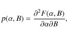
|
(A.2) |
with
| (A.3) |
The joint distribution function satisfies
The function
![]() satisfies
satisfies
![]() and the
normalization condition
and the
normalization condition
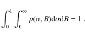
|
(A.4) |
Starting from
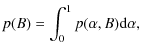
|
(A.5) | ||
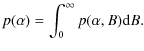
|
(A.6) |
These functions are the PDFs of B and
|
(A.7) | |
|
(A.8) |
They can be used to define the mean values
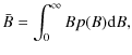
|
(A.9) | |
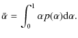
|
(A.10) |
Very useful are the conditional PDFs
| (A.11) | ||
| (A.12) |
With these conditional PDFs, one can define conditional averages,
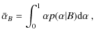
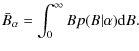
It is easy to verify that
|
(A.15) | ||

|
(A.16) |
The conditional average
The concepts of joint PDF and conditional PDF are easy to grasp with a
graphic representation. We introduce a rectangular coordinate system
![]() ,
with the axes
,
with the axes ![]() and B defining the horizontal
plane and z the vertical axis. The joint PDF defines a surface
and B defining the horizontal
plane and z the vertical axis. The joint PDF defines a surface
![]() .
If we intersect this surface by the vertical plane B=B1, we
obtain the profile of the conditional PDF
.
If we intersect this surface by the vertical plane B=B1, we
obtain the profile of the conditional PDF
![]() ,
as a function
of
,
as a function
of ![]() .
Similarly, a cut by the vertical plane
.
Similarly, a cut by the vertical plane
![]() yields the profile of the conditional PDF
yields the profile of the conditional PDF
![]() ,
as a function
of B.
,
as a function
of B.
In some spectro-polarimetric analysis one considers that the magnetic field
is present everywhere in the medium. In this case the random variable ![]() takes only the value
takes only the value ![]() .
All the expressions given above
hold with
.
All the expressions given above
hold with
![]() ,
,
![]() being the Dirac
distribution. The conditional PDFs become
being the Dirac
distribution. The conditional PDFs become
![]() and
and
![]() .
For the Hanle effect, it is always assumed that
.
For the Hanle effect, it is always assumed that ![]() and often that the magnetic strength has a single value B=B0
. The corresponding joint PDF reduces to
and often that the magnetic strength has a single value B=B0
. The corresponding joint PDF reduces to
![]() .
.
For simplicity in the notation, we have retained the strength B of the
magnetic field as random variable. It is clear that all the definitions
remain the same if we replace B by the magnetic field vector ![]() .
The vector
.
The vector ![]() corresponds actually to three random variables, one for
the strength and two for the direction. The differential element
corresponds actually to three random variables, one for
the strength and two for the direction. The differential element ![]() should be replaced
should be replaced
![]() ,
with
,
with ![]() and
and ![]() the
polar angles of the magnetic field direction in an appropriate reference
frame.
the
polar angles of the magnetic field direction in an appropriate reference
frame.
An interesting quantity for the understanding of the Sun global energy
budget is the mean magnetic energy density in the quiet internetwork. If the
magnetic field is present everywhere, this mean energy is
![]() with
with
|
(A.17) |
If the field is not volume-filling, one should use
|
(A.18) |
This expression can be written
with
| C(B) | = | 
|
|
| = | 
|
(A.20) | |
| = |
Here,
In the analysis of real data, the number N of pixels is not infinite. Also
the magnetic field and filling factor are determined with some error bar.
What is usually inferred from the data are histograms of the
count number, i.e. of the number of
pixels n(Bi) in which the magnetic field strength takes a value between
Bi and
![]() .
Similarly histograms are being
constructed with the number of pixels
.
Similarly histograms are being
constructed with the number of pixels
![]() in which the filling
factor takes a value between
in which the filling
factor takes a value between
![]() and
and
![]() .
The envelopes of these histograms, divided by
.
The envelopes of these histograms, divided by ![]() and
and
![]() ,
yield the marginal PDFs p(B) and
,
yield the marginal PDFs p(B) and
![]() ,
in the limit
,
in the limit
![]() ,
,
![]() ,
,
![]() with
with ![]() and
and
![]() constants. One can
also construct 2D-histograms corresponding to the joint PDF
constants. One can
also construct 2D-histograms corresponding to the joint PDF
![]() .
In each cell
.
In each cell
![]() ,
one plots on the vertical axis, the number of pixels in
which B has a value in the interval
,
one plots on the vertical axis, the number of pixels in
which B has a value in the interval
![]() and
and ![]() has a value in the interval
has a value in the interval
![]() .
As in the continuous case, the conditional histograms are obtained by
cutting the 2D-histogram with vertical planes. Examples of 1D and 2D
histograms can be found in the present paper.
.
As in the continuous case, the conditional histograms are obtained by
cutting the 2D-histogram with vertical planes. Examples of 1D and 2D
histograms can be found in the present paper.
The mean magnetic energy takes the form
|
(A.21) |
with
![$\displaystyle \left[ \sum_{j}\alpha _{j}\frac{n(\alpha _{j},B_{i})}{%
n(B_{i})\Delta \alpha }\Delta \alpha \right] \left[ \frac{n(B_{i})}{N\Delta B}\right] ,$](/articles/aa/full_html/2009/42/aa11373-08/img189.png)
where
Footnotes
- ... THEMIS
- Based on observations made with the French-Italian telescope THEMIS operated by the CNRS and CNR on the island of Tenerife in the Spanish Observatorio del Teide of the Instituto de Astrofísica de Canarias.
- ...
- Present address: Instituto de Astrofísica de Canarias, vía Láctea s/n, 38205 La Laguna, Tenerife, Spain.
All Tables
Table 1: Information on the averaged data. Each line of the table corresponds to one average.
All Figures
|
|
Figure 1: UNNOFIT fit (dotted
line) of a typical observation (full line). The main spectral line
(centered at pixel 38), that is polarized, is Fe I 6302.5 Å,
and the other line, unpolarized, is a telluric line. 10 pixels are
72 mÅ and blue is towards the left. Derived magnetic field
parameters: local average field strength |
| Open with DEXTER | |
| In the text | |
|
|
Figure 2:
Histogram of the local average longitudinal magnetic field (the product of the longitudinal magnetic field Bz with the magnetic filling
factor |
| Open with DEXTER | |
| In the text | |
|
|
Figure 3:
Histogram of the local average magnetic field strength (the product of the magnetic field strength B with the magnetic filling factor |
| Open with DEXTER | |
| In the text | |
|
|
Figure 4: Histogram of the magnetic field inclination with respect to the line-of-sight, from the UNNOFIT inversion. The line-of-sight is also the solar vertical with the observation performed at disk center. |
| Open with DEXTER | |
| In the text | |
|
|
Figure 5: Histogram of the magnetic field azimuth with respect to the slit direction, from the UNNOFIT inversion (ambiguity is not resolved). The observation was performed at disk center and the slit was solar north, so that this is also the histogram of the horizontal field component azimuth. |
| Open with DEXTER | |
| In the text | |
|
|
Figure 6:
Test of the determination of the local average magnetic field strength (the product of the magnetic field strength B with the magnetic filling factor |
| Open with DEXTER | |
| In the text | |
|
|
Figure 7:
Fit of the local average longitudinal magnetic field histogram of Fig. 2 by a Gaussian
|
| Open with DEXTER | |
| In the text | |
|
|
Figure 8:
Fit of the local average magnetic field strength histogram of Fig. 3 by a Maxwellian
|
| Open with DEXTER | |
| In the text | |
|
|
Figure 9:
Test of the determination of the magnetic filling factor by applying Eq. (6)
to the polarimetric data. For the test, the polarimetric data were
theoretical profiles computed from the Unno-Rachkovsky solution,
weighted by a theoretical input magnetic filling factor |
| Open with DEXTER | |
| In the text | |
|
|
Figure 10: Histogram of the filling factor, determined from the polarization data complemented by the UNNOFIT inversion results on the field inclination (see Eq. (6)). The abscissa is in logarithmic scale. |
| Open with DEXTER | |
| In the text | |
|
|
Figure 11:
Histogram of the magnetic field strength, derived by dividing the local average magnetic field strength |
| Open with DEXTER | |
| In the text | |
|
|
Figure 12:
Behavior of the magnetic filling factor |
| Open with DEXTER | |
| In the text | |
|
|
Figure 13:
2D histogram of the magnetic filling factor and of the magnetic field strength B, each pair of them known in each solar pixel. This figure is a 3D representation of the number of points in Fig. 12. The joint PDF
|
| Open with DEXTER | |
| In the text | |
|
|
Figure 14:
Weighted histogram of the magnetic field strength. For each bin of the magnetic field strength histogram of Fig. 11, the count number has been multiplied by the average magnetic field filling factor for this magnetic field strength
|
| Open with DEXTER | |
| In the text | |
|
|
Figure 15: Fit of magnetic field strength histogram of Fig. 11 by the magnetic field PDF p(B) derived from the linear fits of Figs. 12 and 14. This magnetic field PDF is given by Eq. (18). |
| Open with DEXTER | |
| In the text | |
|
|
Figure 16: Same as Fig. 7, but with the number of pixels per bin (counts) plotted on a logarithmic scale to highlight the distribution in the wings. |
| Open with DEXTER | |
| In the text | |
Copyright ESO 2009
Current usage metrics show cumulative count of Article Views (full-text article views including HTML views, PDF and ePub downloads, according to the available data) and Abstracts Views on Vision4Press platform.
Data correspond to usage on the plateform after 2015. The current usage metrics is available 48-96 hours after online publication and is updated daily on week days.
Initial download of the metrics may take a while.