| Issue |
A&A
Volume 506, Number 2, November I 2009
|
|
|---|---|---|
| Page(s) | 885 - 893 | |
| Section | The Sun | |
| DOI | https://doi.org/10.1051/0004-6361/200912652 | |
| Published online | 18 August 2009 | |
A&A 506, 885-893 (2009)
On the vertical and horizontal transverse oscillations of curved coronal loops
M. S. Ruderman
Department of Applied Mathematics, University of Sheffield, Hicks Building, Hounsfield Road, Sheffield S3 7RH, UK
Received 8 June 2009/ Accepted 10 August 2009
Abstract
Kink oscillations of curved coronal loops with the density varying along the
loop are studied in the thin tube approximation. The equilibrium magnetic field
is assumed to be potential, and the field potential and flux function are used
as curvilinear coordinates. It is also assumed that the loop expansion is weak,
and the solution to the problem is looked for in the form of power series with
respect to the tube expansion parameter
![]() .
The main result of the
study is that the eigenfrequencies of the vertical and horizontal tube
oscillations are, in general, different, their difference being proportional to
.
The main result of the
study is that the eigenfrequencies of the vertical and horizontal tube
oscillations are, in general, different, their difference being proportional to
![]() .
As an example a simple equilibrium with the magnetic field
magnitude exponentially decaying with the height is considered. The implication
of the obtained results for the interpretation of observational data is
discussed.
.
As an example a simple equilibrium with the magnetic field
magnitude exponentially decaying with the height is considered. The implication
of the obtained results for the interpretation of observational data is
discussed.
Key words: magnetohydrodynamics (MHD) - waves - Sun: oscillations - Sun: corona
1 Introduction
Since transverse oscillations of coronal loops were first observed by TRACE (Aschwanden et al. 1999; Nakariakov et al. 1999), they received ample attention from both observers and theorists. The majority of observed transverse oscillations of coronal loops were polarised in the horizontal direction. However, Wang & Solanki (2004) and Wang et al. (2008) reported the observations by TRACE of the vertically polarised transverse oscillations of coronal loops. These observations raise a question: what is the difference between properties of the horizontally and vertically polarised oscillations? In particular, do they have the same frequencies, or their frequencies are different?
In first theoretical studies of transverse oscillations of coronal loops the simplest model of a coronal loop was used. In this model a coronal loop is considered as a straight homogeneous magnetic tube with the footpoints frozen in the dense photospheric plasma. Since this magnetic plasma configuration is axisymmetric, the loop oscillations can be polarised in any direction, and the oscillation frequency is independent of the polarisation direction. Then more complicated models taking such effects as the density variation along and across a loop, the loop expansion and curvature were developed (see review paper by Ruderman & Erdélyi 2009, and references therein). In particular, Van Doorsselaere et al. (2004) considered transverse oscillations of curved coronal loops. They assumed that the loop has the form of a half-circle and neglected the coronal density stratification. Using the toroidal coordinates they studied the transverse loop oscillations in the thin tube approximation. Their conclusion was that the eigenmode frequencies of the transverse loop oscillations remain unchanged up to first order in curvature. The curvature has more pronounced effect on the damping rate caused by resonant absorption in a thin boundary layer near the tube boundary. The correction to the damping rate due to the curvature is of the first order in curvature.
Later Terradas et al. (2006) studied the same problem as Van Doorsselaere et al. (2004), however taking the density stratification into account. Since Terradas et al. (2006) did not use the thin tube approximation but rather solved the exact linearised MHD equations, they managed to calculate corrections to the oscillation frequencies due to curvature. As a result, they found that the curvature removes the degeneration of eigenmodes of the transverse loop oscillations in a sense that now the eigenmodes can be polarised either in the horizontal or in the vertical direction only. However for thin coronal loops the difference between the eigenfrequencies of the two modes is very small.
Terradas et al. (2006) also studied the damping of transverse oscillations. In contrast to Van Doorsselaere et al. (2004) they did not assume that the inhomogeneous layer where the density varies in the radial direction is thin. Rather they allowed the density to vary in a layer with an arbitrary thickness. Terradas et al. (2006) confirmed the conclusion by Van Doorsselaere et al. (2004) that curvature has mode pronounced effect on the damping rate than on the eigenfrequencies. In addition, they found that, due to the density stratification, the oscillations become leaky and can be in resonance with the local Alfvén oscillations in the external plasmas. However the damping due to resonant absorption in the boundary layer near the tube boundary strongly dominates the damping due to leakage and resonance in the external plasma.
A very important assumption made by both Van Doorsselaere et al. (2004) and Terradas et al. (2006) was that the loop cross-section is circular and its radius does not very along the loop. These conditions are hardly satisfied in real coronal loops. The loop expansion leads to the variation of the loop cross-section area along the loop. In addition, the loop curvature can cause the variation of the cross-section shape. In this paper we study the effect of the variation of the loop cross-section on the transverse coronal loop oscillations using a simple model where the loop is embedded in a two-dimensional potential magnetic field. The paper is organised as follows. In the next section we formulate the problem, describe the unperturbed state, and present the governing equations in curvilinear coordinates. In Sect. 3 we simplify the governing equations using the thin tube approximation. In Sect. 4 we study the eigenmodes of the vertical and horizontal loop oscillations in the approximation of weak tube expansion. In Sect. 5 we apply general results obtained in the previous sections to a particular equilibrium with exponentially decaying magnetic field. Section 6 presents the summary of the obtained results and our conclusions.
2 Problem formulation and governing equations
Let us introduce Cartesian coordinates x, y, z with the z-axis in the
vertical direction, and consider an
equilibrium magnetic field ![]() with the magnetic field lines in the
xz-plane that is independent of y. Since the magnetic field is
solenoidal, it follows that
with the magnetic field lines in the
xz-plane that is independent of y. Since the magnetic field is
solenoidal, it follows that ![]() can be expressed in terms of magnetic flux
function
can be expressed in terms of magnetic flux
function ![]() .
We also assume that
.
We also assume that ![]() is potential, so that it can
be expressed in terms of potential
is potential, so that it can
be expressed in terms of potential ![]() .
As a result we have
.
As a result we have
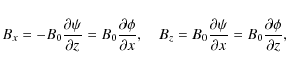
where B0 is the characteristic value of the equilibrium magnetic field. We assume that the magnetic field is closed with the footpoints of the magnetic field lines frozen in the dense photospheric plasma. The sketch of a typical equilibrium state is shown in Fig. 1.
![\begin{figure}
\par\includegraphics[width=8cm,clip]{fig1.eps}
\end{figure}](/articles/aa/full_html/2009/41/aa12652-09/img7.png) |
Figure 1: The sketch of the equilibrium state. The ends of the magnetic loop are assumed to be frozen in a dense photospheric plasma. The axis of the magnetic loop is shown by the thick line. A few cross-sections of the loop are shown by ellipses. |
| Open with DEXTER | |
A magnetic field line is determined by the equations
![]() and
and
![]() .
The equation of the loop axis is
.
The equation of the loop axis is
![]() ,
where
,
where
![]() is a constant. We assume that this axis is in the xz-plane. The
equation of the loop boundary can be written in a parametric form as
is a constant. We assume that this axis is in the xz-plane. The
equation of the loop boundary can be written in a parametric form as
![]() ,
,
![]() ,
where
,
where
![]() and
and
![]() .
The
interior of the loop is defined by the equation
.
The
interior of the loop is defined by the equation
![\begin{displaymath}(\psi - \psi_0)^2 + y^2 < [\psi(\eta) - \psi_0]^2 + y^2(\eta) ,
\end{displaymath}](/articles/aa/full_html/2009/41/aa12652-09/img16.png)
while its exterior is defined by the equation
![\begin{displaymath}(\psi - \psi_0)^2 + y^2 > [\psi(\eta) - \psi_0]^2 + y^2(\eta) .
\end{displaymath}](/articles/aa/full_html/2009/41/aa12652-09/img17.png)
We assume that the plasma density,
The plasma motion is described by linearised ideal MHD equations for cold
plasmas,
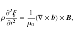
Here
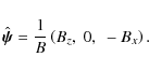
Now we introduce the curvilinear coordinates
![]() .
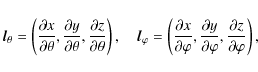
The unit
vectors in this coordinate system are
.
The unit
vectors in this coordinate system are
![]() ,
,
![]() and
and
![]() .
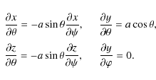
It follows from Eq. (1) that
.
It follows from Eq. (1) that
![]() ,
and the Cartesian
components of
,
and the Cartesian
components of
![]() are given by
are given by
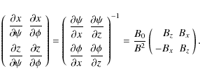
It is straightforward to see that the introduced curvilinear coordinate system is orthogonal and right-oriented (
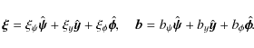
Let us introduce the components of vectors
Then, using Eq. (5), the expression for the operator
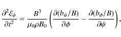
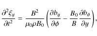
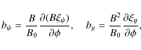
where

where
where
The system of Eqs. (10)-(12) with the boundary conditions (13) and (14) is used in what follows to study the fast kink oscillations of curved coronal loops.
3 Thin-tube approximation
Let L be the loop length and a be the characteristic size of loop
cross-sections. For typical coronal loops ![]() ,
which inspires us to
introduce
,
which inspires us to
introduce
![]() .
To have the same spatial scales of
perturbation variation with respect to all three variables,
.
To have the same spatial scales of
perturbation variation with respect to all three variables, ![]() ,
y and
,
y and ![]() ,
we introduce the new scaled variable
,
we introduce the new scaled variable
![]() .
Since
the characteristic period of kink oscillations is equal to the transverse
Alfvén time times L/a, we also introduce the scaled time
.
Since
the characteristic period of kink oscillations is equal to the transverse
Alfvén time times L/a, we also introduce the scaled time
![]() .
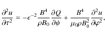
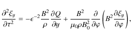
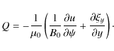
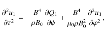
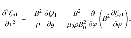
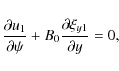
In new variables Eqs. (10)-(12) are rewritten as
.
In new variables Eqs. (10)-(12) are rewritten as
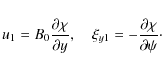
Now we look for solution to this system of equations in the form of expansions with respect to
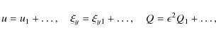
where the dots indicate terms of higher order with respect to
Substituting Eqs. (18) and (19) in Eqs. (15)-(17), and collecting terms of the lowest order with respect to
where B is calculated at
Substituting these expressions in Eqs. (20) and (21), and using cross-differentiation to eliminate Q1, we obtain the following equation for
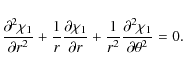
Let us introduce the polar coordinates in the
(recall that
where
In what follows we assume that the loop boundary is determined by the equation
r = a. In the first order approximation with respect to ![]() the
quantities
the
quantities ![]() and
and ![]() are related by
are related by
Hence, once again in the first order approximation with respect to
This is the equation of an ellipse with the half-axes equal to a and a(B0/B), where B is calculated at the loop axis. We see that, while the axis parallel to the y-direction is constant, the perpendicular axis, in general, varies along the loop.
In what follows we are looking for eigenmodes of the loop oscillations and take
perturbations of all quantities proportional to
![]() .
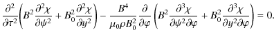
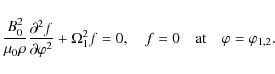
Then, in the new variables, Eq. (24) takes the form
.
Then, in the new variables, Eq. (24) takes the form
![\begin{displaymath}\frac{B^4}{\mu_0\rho B_0^2}\frac{\partial}{\partial\varphi}
...
...al\chi}{\partial\varphi}\right]
+ \Omega^2{\cal L}[\chi] = 0,
\end{displaymath}](/articles/aa/full_html/2009/41/aa12652-09/img86.png)
where
The expression for
Let us now rewrite the boundary conditions (13) in terms of ![]() .
To transform the first boundary condition we need to calculate the normal vector
to the loop boundary. Since r = a at the boundary, and the Cartesian
coordinates of a point are functions of
.
To transform the first boundary condition we need to calculate the normal vector
to the loop boundary. Since r = a at the boundary, and the Cartesian
coordinates of a point are functions of ![]() ,
y and
,
y and ![]() ,
the
equation of the boundary in Cartesian coordinates can be written as
,
the
equation of the boundary in Cartesian coordinates can be written as
![\begin{displaymath}\begin{array}{l}
x = x(\psi_0 + a\cos\theta,\varphi), \\ [2mm...
...heta, \\ [2mm]
z = z(\psi_0 + a\cos\theta,\varphi).
\end{array}\end{displaymath}](/articles/aa/full_html/2009/41/aa12652-09/img95.png)
Here we have taken into account that x and z are functions of
are tangential to the boundary. To evaluate these vectors we use the relations
We obtain with the aid of Eq. (1) that
Using this result, Eq. (30), and the relation between
The unit normal vector to the boundary is then given by

where
When deriving this expression we have used Eq. (4). The normal component of the displacement is given by
| |
= | ||
| = |  |
This expression is only valid in the lowest order approximation with respect to
To rewrite the second boundary condition in (13) in terms of
![\begin{displaymath}\left[\frac{B^4}{\mu_0 B_0^2}\frac{\partial}{\partial\varphi}...
...\Omega^2{\cal M}[\chi]\right] = 0 \quad \mbox{at} \quad r = a,
\end{displaymath}](/articles/aa/full_html/2009/41/aa12652-09/img112.png)
where
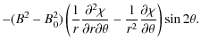
![\begin{displaymath}{\cal M}[\chi] = (B^2\cos^2\theta + B_0^2\sin^2\theta)
\frac...
... - B_0^2)}{2a}\frac{\partial\chi}{\partial\theta}\sin2\theta ,
\end{displaymath}](/articles/aa/full_html/2009/41/aa12652-09/img113.png)
and the expression for
Finally, it follows from (14) and (23) that ![]() is
constant at
is
constant at
![]() .
Since
.
Since ![]() is determined with the
accuracy up to an additive function of
is determined with the
accuracy up to an additive function of ![]() ,
we can take
,
we can take
4 Eigenmodes of weakly expanding loops
To make analytical progress we consider weakly expanding loops and assume that
the variation of the magnetic field magnitude along the loop is small. In
accordance with this assumption we take
![\begin{displaymath}B^2 = B_0^2[1 + \lambda q(\varphi)] ,
\end{displaymath}](/articles/aa/full_html/2009/41/aa12652-09/img118.png)
and assume that
4.1 First order approximation
In the first order approximation we substitute the expansions (36)
and (37) in Eq. (26), and boundary conditions
(32), (33) and (35). As a result we obtain
![\begin{displaymath}[\chi_1]= \left[\left(\frac{B_0^2}{\mu_0}\frac{\partial^2}
{...
...\chi_1}
{\partial r}\right] = 0 \quad \mbox{at} \quad r = a ,
\end{displaymath}](/articles/aa/full_html/2009/41/aa12652-09/img122.png)
If we denote the expression in the second brackets in Eq. (38) as f, then it follows from Eq. (40) that f = 0 at
Since
In what follows we only study the kink oscillations, so that we take
Substituting this expression in Eq. (42) we obtain
In addition, the functions
Substituting this solution in the second boundary condition in (39) yields
This equation coincides with the equation derived by Dymova & Ruderman (2005) for kink oscillations of a straight loop with the constant circular cross-section. This is not surprising at all because, in the first order approximation with respect to
Equation (46) and the boundary condition (47) constitute the Sturm-Liouville problem. This problem has a non-trivial solution only when
where
4.2 Second order approximation
In the second order approximation we collect terms proportional to ![]() in
Eq. (26), and boundary conditions (32),
(33) and (35). Then, using (43),
(45), (46) and (48), we obtain
in
Eq. (26), and boundary conditions (32),
(33) and (35). Then, using (43),
(45), (46) and (48), we obtain


![$\displaystyle \bigg[\bigg(\displaystyle\frac{B_0^2}{\mu_0}\frac{\partial^2}
{\partial\varphi^2} + \rho\Omega_1^2\bigg)
\frac{\partial\chi_2}{\partial r}\bigg]$](/articles/aa/full_html/2009/41/aa12652-09/img151.png)

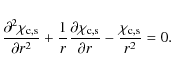
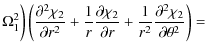
Equation (49) for
where
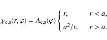
We look for the solution to Eq. (50) in the form
Substituting this expression in Eq. (50) we obtain
The general solution to this equation is given by
where
Substituting (55) in (51) and using (57) we obtain
It follows from (53) that
Now we substitute (54) and (59) in the boundary condition (52), and collect terms proportional to
![]() ,
,
![]() ,
and
,
and
![]() .
As a result we obtain
equations for
.
As a result we obtain
equations for
![]() ,
,
![]() ,
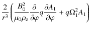
and A3. The equation for A3coincides with (58), and the equations for A2c and A2s are
,
and A3. The equation for A3coincides with (58), and the equations for A2c and A2s are

The homogeneous counterparts to Eqs. (60) and (61) coincide with Eq. (49), so that they have a non-trivial solution
![$\displaystyle \left.+ 3\rho_{\rm e})A_1^2 + \frac3{\Omega_1}
\left(\frac{{\rm d}A_1}{{\rm d}\varphi}\right)^2\right]~{\rm d}\varphi ,$](/articles/aa/full_html/2009/41/aa12652-09/img192.png)
![$\displaystyle \left. + 3\rho_{\rm e})A_1^2 + \frac1{\Omega_1}
\left(\frac{{\rm d}A_1}{{\rm d}\varphi}\right)^2\right]~{\rm d}\varphi .$](/articles/aa/full_html/2009/41/aa12652-09/img194.png)
In general,
This result implies that the case where
4.3 Equations in physical variables
In the first order approximation with respect to ![]() the eigenfrequencies
and eigenmodes of the loop kink oscillations are determined by Eq. (46) with the boundary conditions (47). The second order
corrections to the eigenfrequencies are given by Eqs. (62) and
(63). All these equations are written in variables that are
inconvenient for comparison with the results obtained in previous studies and
with observations. We now rewrite these equations in physical variables. We
start from introducing the length s along the loop axis. Since
the eigenfrequencies
and eigenmodes of the loop kink oscillations are determined by Eq. (46) with the boundary conditions (47). The second order
corrections to the eigenfrequencies are given by Eqs. (62) and
(63). All these equations are written in variables that are
inconvenient for comparison with the results obtained in previous studies and
with observations. We now rewrite these equations in physical variables. We
start from introducing the length s along the loop axis. Since
![]() ,
we obtain
,
we obtain
![]() ,
so that
,
so that
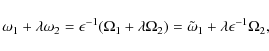
We also introduce
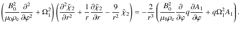
where L is the length of the loop given by
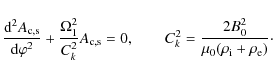
and either
where either
In the next order approximation we obtain
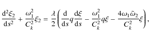
with
![\begin{displaymath}\tilde{\omega}_2\int_0^L \frac{\xi^2}{C_k^2}~{\rm d}\xi = -\f...
...s}\right)^2 +
\frac{\omega_1^2}{C_k^2}\xi^2\right]{\rm d}s .
\end{displaymath}](/articles/aa/full_html/2009/41/aa12652-09/img219.png)
Now we introduce
so that
where

![$\displaystyle \int_0^L\frac q8\left[\frac{\mu_0\omega_1}{B_0^2}
(3\rho_{\rm i} ...
...- \frac1{\omega_1}
\left(\frac{{\rm d}\xi}{{\rm d}s}\right)^2\right]~{\rm d}s ,$](/articles/aa/full_html/2009/41/aa12652-09/img229.png)

![$\displaystyle \int_0^L\frac q8\left[\frac{\mu_0\omega_1}{B_0^2}
(\rho_{\rm i} +...
...+ \frac1{\omega_1}
\left(\frac{{\rm d}\xi}{{\rm d}s}\right)^2\right]~{\rm d}s .$](/articles/aa/full_html/2009/41/aa12652-09/img231.png)
To verify the correctness of the obtained results we consider kink oscillations of a straight homogeneous magnetic tube with an elliptic cross-section. To do this we take q to be a non-zero constant. Then the half-axes of the elliptic cross-section are a and
Kink oscillations of a straight homogeneous magnetic tube with an elliptic cross-section were studied by Ruderman (2003). In particular, he obtained the expressions for the frequencies of two kink modes in the thin tube approximation (see his Eq. (60)). If we substitute
5 Exponentially decaying magnetic field in an isothermal atmosphere
To give an example of the obtained general results we consider the following
equilibrium state. The potential and flux function of the equilibrium magnetic
field are give by
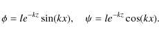
The picture of the field lines for this magnetic field is qualitatively the same as one shown in Fig. 1. The ratio of densities inside and outside the loop is constant,

where H is the atmospheric scale height. The loop footpoints are at z = 0,
Using (74) and (76) we can express z in terms of
It follows from (1) and (74) that
so that
This equation implies that
The function
It follows from the second equation in (81) that

in what follows. To satisfy the first Eq. in (81) we take
where
Now we can rewrite the equation of the loop axis (76) in an approximate form,
![\begin{displaymath}z = \frac12 x_0\sqrt{\lambda}\left[1 - \left(\frac x{x_0}\right)^2\right] \cdot
\end{displaymath}](/articles/aa/full_html/2009/41/aa12652-09/img260.png)
We see that the loop shape is approximately parabolic. The ratio of the loop height to the distance between the loop footpoints is
The loop cross-section is elliptic with the horizontal half-axis equal to a.
The vertical half-axis is equal to
![]() .
Hence, in accordance with (74) and (82)-(84),
it monotonically increases with the height from
.
Hence, in accordance with (74) and (82)-(84),
it monotonically increases with the height from
![]() at the
loop footpoints to
at the
loop footpoints to
![]() at the loop apex.
at the loop apex.
The distance along the loop is related to the magnetic field potential by
Eq. (65). Using (74), (79) and
(84) we obtain from this equation
![$\displaystyle \int_{-x_0[1 + (\alpha-1/6)\lambda]}^\phi\left[1
- \frac\lambda2\left(x_0^{-2}{\phi'}^2 + 2\alpha - 1\right)\right]{\rm d}\phi'$](/articles/aa/full_html/2009/41/aa12652-09/img266.png)
![$\displaystyle \phi + x_0 + \lambda\left[\left(\alpha-\frac16\right)x_0
- \frac{\phi^3 + x_0^3}{6x_0^2}
- \left(\alpha-\frac12\right)(\phi + x_0)\right] .$](/articles/aa/full_html/2009/41/aa12652-09/img267.png)
Substituting
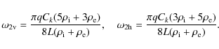
Now we assume that H and L are of the same order of magnitude. Since the loop height is of the order of
where
![\begin{displaymath}\omega_{2\rm v} = \frac{C_k[\pi^2(5\zeta+3)(6\alpha+1) - 6(7\zeta+5)]}
{24\pi^2 L(\zeta+1)} ,
\end{displaymath}](/articles/aa/full_html/2009/41/aa12652-09/img277.png)
![\begin{displaymath}\omega_{2\rm h} = \frac{C_k[\pi^2(3\zeta+5)(6\alpha+1) - 6(\zeta+3)]}
{24\pi^2 L(\zeta+1)} \cdot
\end{displaymath}](/articles/aa/full_html/2009/41/aa12652-09/img278.png)
When deriving these expressions we have taken
![$\displaystyle \frac{\lambda C_k[\pi^2(\zeta-1)(6\alpha+1) - 6(3\zeta+1)]}
{12\pi^2 L(\zeta+1)}\cdot$](/articles/aa/full_html/2009/41/aa12652-09/img282.png)
We see that, in general,
It is especially instructive to take
so that
6 Summary and conclusions
In this paper we have studied kink oscillations of curved coronal magnetic loops with the density varying along the loop. We have assumed that the loop is in a vertical plane, so that the loop torsion is zero. We have also assumed that the equilibrium magnetic field is potential. Using the magnetic field potential and flux function as curvilinear coordinates in the loop plane we derived the equation governing the loop motion in the thin tube approximation. Then we have considered a loop with the elliptic cross-section, and rewrote the governing equations and the boundary conditions at the loop boundary in terms of polar coordinates in the loop cross-section. An important property of this model is that the loop curvature causes the loop expansion. As a result the ratio of axis of the loop cross-section varies along the loop.
The governing equation for the loop motion is a partial differential equation
for one function that depends of the polar coordinates in the loop
cross-section, r and ![]() .
The coefficients of this equation depend both
on r and
.
The coefficients of this equation depend both
on r and ![]() .
We managed to find the solution to the governing equation
corresponding to kink oscillations inside the loop. However, it seems highly
improbable that a similar solution describing the motion outside the loop can be
found. To make analytical progress we assumed that the loop expansion is small
and introduced the small parameter,
.
We managed to find the solution to the governing equation
corresponding to kink oscillations inside the loop. However, it seems highly
improbable that a similar solution describing the motion outside the loop can be
found. To make analytical progress we assumed that the loop expansion is small
and introduced the small parameter, ![]() ,
characterising this expansion.
In this approximation the loop cross-section is almost circular. The ratio of
axes of the loop elliptic cross-section differs from unity by a quantity of the
order of
,
characterising this expansion.
In this approximation the loop cross-section is almost circular. The ratio of
axes of the loop elliptic cross-section differs from unity by a quantity of the
order of ![]() .
After that we have used the regular perturbation method
and looked for the solution to the problem in the form of power series
expansions with respect to
.
After that we have used the regular perturbation method
and looked for the solution to the problem in the form of power series
expansions with respect to ![]() .
.
In particular, we looked for the eigenmodes of kink oscillations in the form
![]() .
In the first order approximation we
found that
.
In the first order approximation we
found that ![]() is determined by the eigenvalue problem
(68). Equation (68) is exactly the same as one obtained by
Dymova & Ruderman (2005) for kink oscillations of a straight non-expanding loop with the
circular cross-section and the density varying along the loop. The eigenvalue
problem is degenerate in the sense that kink oscillations can be polarised in
any direction.
is determined by the eigenvalue problem
(68). Equation (68) is exactly the same as one obtained by
Dymova & Ruderman (2005) for kink oscillations of a straight non-expanding loop with the
circular cross-section and the density varying along the loop. The eigenvalue
problem is degenerate in the sense that kink oscillations can be polarised in
any direction.
In the next order approximation the kink eigenmodes of the loop oscillation can be polarised only either in the vertical or horizontal direction, so that the degeneration of the eigenvalue problem is removed. The corrections to the kink oscillation frequency are different for the vertical and horizontal oscillations. They are given by Eqs. (72) and (73) for the fundamental modes of the vertical and horizontal kink oscillations.
As an example we have considered a simple equilibrium with the magnetic field
magnitude exponentially decaying with the height. Neglecting the density
variation along the loop we reduced the eigenvalue problem (68) to
one describing kink oscillations of a straight thin homogeneous magnetic tube.
Then we easily calculated the corrections to the frequencies of the vertical and
horizontal oscillations,
![]() and
and
![]() (see Eqs. (88) and (89)). These corrections depend on the parameter
(see Eqs. (88) and (89)). These corrections depend on the parameter
![]() characterising the shape of the loop cross-section at the footpoints.
In general, this cross-section is an ellipse with the ration of the vertical and
horizontal axes equal to
characterising the shape of the loop cross-section at the footpoints.
In general, this cross-section is an ellipse with the ration of the vertical and
horizontal axes equal to
![]() .
When
.
When
![]() ,
which
corresponds to the circular footpoint cross-section,
,
which
corresponds to the circular footpoint cross-section,
![]() ,
i.e. the frequency of the vertical loop
oscillation is smaller than that of the horizontal oscillation.
,
i.e. the frequency of the vertical loop
oscillation is smaller than that of the horizontal oscillation.
The main conclusion of this work is that the frequencies of the vertical and
horizontal kink oscillations are, in general, different. The effect of loop
curvature on the frequencies of the vertical and horizontal kink oscillations
is not direct. Rather the curvature results in variation of the shape of the
loop cross-section along the loop, and it is this variation of the
cross-section shape that causes the difference in the frequencies. It is
instructive to compare the results of this work with those obtained by
Van Doorsselaere et al. (2004) and Terradas et al. (2006). These authors came to a conclusion that the
difference between the frequencies of the vertical and horizontal oscillations
of a curved loop is only of the order of
![]() ,
where
,
where ![]() is
the ration of the loop radius to its length, so that it can be neglect in the
thin tube approximation. Our study clearly shows that this result in related
to the model used by Van Doorsselaere et al. (2004) and Terradas et al. (2006). In this model a curved
loop has a circular cross-section with the constant radius.
is
the ration of the loop radius to its length, so that it can be neglect in the
thin tube approximation. Our study clearly shows that this result in related
to the model used by Van Doorsselaere et al. (2004) and Terradas et al. (2006). In this model a curved
loop has a circular cross-section with the constant radius.
The difference between the frequencies of the vertical and horizontal
oscillations is of the order of
![]() ,
i.e. it is small. This result
is directly related to our assumption that the loop expansion is small. For
loops with sufficiently large expansions this difference can be quite
substantial.
,
i.e. it is small. This result
is directly related to our assumption that the loop expansion is small. For
loops with sufficiently large expansions this difference can be quite
substantial.
Although, as we have already mentioned, the majority of observed kink oscillations of coronal loops are horizontally polarised, an arbitrary disturbance should cause both vertically and horizontally polarised oscillations. Since, in general, the frequencies of the vertical and horizontal oscillations are different, it would be interesting to look for signatures of two different frequencies in the observational data. If the ratio of two observed frequencies is sufficiently large (say, larger than 1.5), then they are usually attributed to the fundamental mode and first overtone of kink oscillations. However if two frequencies with a smaller ratio (say, 1.2 or 1.3) are found, then it is quite probable that they are the frequencies of the vertical and horizontal kink oscillations.
AcknowledgementsThe author acknowledges support by an STFC grant.
References
- Aschwanden, M. J., Fletcher, L., Schrijver, C. J., & Alexander, D. 1999, ApJ, 520, 880 [NASA ADS] [CrossRef]
- Dymova, M., & Ruderman, M. S. 2005, Sol. Phys., 229, 79 [NASA ADS] [CrossRef]
- Korn, G. A., & Korn, T. M. 1961, Mathematical handbook for scientists and engineers (New York: McGraw-Hill)
- Nakariakov, V. M., Ofman, L., DeLuca, E. E., Roberts, B., & Davila, J. M. 1999, Science, 285, 862 [NASA ADS] [CrossRef]
- Ruderman, M. S. 2003, A&A, 409, 287 [NASA ADS] [CrossRef] [EDP Sciences]
- Ruderman, M. S., & Erdélyi, R., Space. Sci. Rev., in press
- Terradas, J., Oliver, R., & Ballester, J. L. 2006, ApJ, 650, L91 [NASA ADS] [CrossRef]
- Van Doorsselaere, T., Debosscher, A., Andries, J., & Poedts, S. 2004, A&A, 424, 1065 [NASA ADS] [CrossRef] [EDP Sciences]
- Wang, T. J., & Solanki, S. K. 2004, A&A, 421, L33 [NASA ADS] [CrossRef] [EDP Sciences]
- Wang, T. J., Solanki, S. K., & Selwa, M. 2008, A&A, 489, 1307 [NASA ADS] [CrossRef] [EDP Sciences]
All Figures
| |
Figure 1: The sketch of the equilibrium state. The ends of the magnetic loop are assumed to be frozen in a dense photospheric plasma. The axis of the magnetic loop is shown by the thick line. A few cross-sections of the loop are shown by ellipses. |
| Open with DEXTER | |
| In the text | |
Copyright ESO 2009
Current usage metrics show cumulative count of Article Views (full-text article views including HTML views, PDF and ePub downloads, according to the available data) and Abstracts Views on Vision4Press platform.
Data correspond to usage on the plateform after 2015. The current usage metrics is available 48-96 hours after online publication and is updated daily on week days.
Initial download of the metrics may take a while.