| Issue |
A&A
Volume 506, Number 1, October IV 2009
The CoRoT space mission: early results
|
|
|---|---|---|
| Page(s) | 153 - 158 | |
| Section | Stellar structure and evolution | |
| DOI | https://doi.org/10.1051/0004-6361/200911893 | |
| Published online | 16 July 2009 | |
The CoRoT space mission: early results
Accuracy of stellar parameters of exoplanet-host stars determined from asteroseismology
C. Mulet-Marquis1 - I. Baraffe1 - S. Aigrain2 - F. Pont2
1 - C.R.A.L, CNRS, UMR5574
École normale supérieure, 46 allée d'Italie, 69007 Lyon, France
2 -
School of Physics, University of Exeter, Stocker Road, Exeter, EX4 4QL, UK
Received 20 February 2009 / Accepted 16 June 2009
Abstract
Context. In the context of the space-based mission CoRoT, devoted to asteroseismology and search for planet transits, we analyse the accuracy of fundamental stellar parameters (mass, radius, luminosity) that can be obtained from asteroseismological data.
Aims. Our work is motivated by the large uncertainties on planetary radius determination of transiting planets which are mainly due to uncertainties on the stellar parameters. Our goal is to analyse uncertainties of fundamental stellar parameters for a given accuracy of oscillation frequency determination.
Methods. We generate grids of equilibrium models of stars and compute their pulsation spectra based on a linear nonadiabatic stability analysis. Using differents methods of comparison of oscillation mode spectra, we derive uncertainties on fundamental stellar parameters and analyse the effect of varying the number of considered modes.
Results. The limits obtained depend strongly on the adapted method to compare spectra. We find a degeneracy in the stellar parameter solutions, up to a few % in mass (from less than 1% to more than 7% depending on the method used and the number of considered modes), luminosity (from 2% to more than 10%) or radius (from less than 1% to 3%), for a given pulsation spectrum.
Key words: stars: oscillations - stars: fundamental parameters
1 Introduction
The successful launching of CoRoT produces data for transiting exoplanets with unprecedented accuracy compared to ground-based observations, providing a measure of planetary mass and radius and thus information on the mean density and bulk composition of exoplanets. Unfortunately, a remaining source of uncertainty on the planetary parameters (mass and radius) is due to uncertainties on the stellar parameters.
The precise determination of gravity by spectroscopy is difficult, and particularly for F stars. The determination of the mass of the star is the main uncertainty on the planet's size. This uncertainty on the mass is generally about 10% (i.e. 3% on the radius and 10% on the density). This may be of importance to disantangle a massive planet from a brown dwarf, as in the case of the recently discovered ``super-Jupiter'' CoRoT-3b (Leconte et al. 2009). It may also prevent distinguishing an ocean planet from an earth-like planet (Grasset et al. 2009).
Our goal is to examine the accuracy on the latter parameters, namely mass, luminosity and radius, that could be obtained using asteroseismology with the expected accuracy on oscillation frequencies of CoRoT. We explore the space of stellar parameters, in terms of mass, effective temperature, luminosity, metallicity and mixing length parameter and we analyse the sensitivity of predicted spectrum of oscillation frequencies to these parameters. Adopting various levels of stellar noise and white noise, we analyse the frequency uncertainty for oscillation modes of a given amplitude and lifetime. This analysis is based on the performances of CoRoT in the Asteroseismology and Planet Finder channels described in Auvergne et al. (2009).
2 Method
2.1 Stars studied
Among all the transiting systems discovered so far, the large difference between the fundamental parameters of XO-3 given by Johns-Krull et al. (2008)
(
![]() ;
;
![]() )
and by Winn et al. (2008)
(
)
and by Winn et al. (2008)
(
![]() ;
;
![]() )
was a strong motivation to examine how accurately fundamental parameters of a star (mass, radius, luminosity) can be
constrained by asteroseismology.
In this preliminary study, we first analyse stars with characteristics close to the ones of XO-3 (
)
was a strong motivation to examine how accurately fundamental parameters of a star (mass, radius, luminosity) can be
constrained by asteroseismology.
In this preliminary study, we first analyse stars with characteristics close to the ones of XO-3 (
![]() ,
,
![]() ,
,
![]() K). We focus on modes with low order l (
K). We focus on modes with low order l (
![]() )
and radial order n between 5 and 20.
)
and radial order n between 5 and 20.
2.2 Frequency computation
The pulsation calculations are performed with a nonradial code originally developed by Lee (1985) and based on a linear non-adiabatic stability analysis.
The equations are linearised around hydrostatic equilibrium, and eigenfunctions are expressed with spherical harmonics
![]() .
The eigenfrequencies are defined by
.
The eigenfrequencies are defined by
| (1) |
with
2.3 Accuracy of frequency determination
The photometric performance of CoRoT, described in Auvergne et al. (2009), allows for the detection and characterisation of Sun-like oscillations of bright (6<V<9) stars in the asteroseismology (AS) channel, and larger amplitude red giant pulsations on fainter (V>11.5) stars in the planet finding (PF) channel.
The precision to which mode frequencies can be determined depends on
the mode lifetime ![]() ,
the duration T of the dataset, the mode
amplitude A and the background, power density B (including stellar
and white noise) at the frequency of the mode. In the case of both
Sun-like and red giant oscillations, mode lifetimes are of the order
of a few days (Fletcher et al. 2006), much shorter than a typical CoRoT run (21
or 150 days). We therefore use the formula given by Libbrecht (1992) for
the case where
,
the duration T of the dataset, the mode
amplitude A and the background, power density B (including stellar
and white noise) at the frequency of the mode. In the case of both
Sun-like and red giant oscillations, mode lifetimes are of the order
of a few days (Fletcher et al. 2006), much shorter than a typical CoRoT run (21
or 150 days). We therefore use the formula given by Libbrecht (1992) for
the case where
![]() to estimate the frequency uncertainty
to estimate the frequency uncertainty
![]() as:
as:

where
![\begin{displaymath}f(\beta) = \left( 1 + \beta \right)^{1/2}
\left[ \left(1 + \beta \right)^{1/2} + \beta^{1/2} \right]^3.
\end{displaymath}](/articles/aa/full_html/2009/40/aa11893-09/img31.png)
As is common practice in asteroseismology (see e.g. Kallinger et al. 2009, and references therein), we model B as a sum of broken power-laws of the form
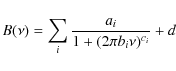
where each term in the sum corresponds to the stellar variability associated with a particular type of surface structure (typically active regions and granulation, with in some cases a super-granulation component), ai is the amplitude, bi the characteristic time-scale, and ci the slope of term i, and d represents the white noise.
Table 1:
Parameters of the background models used. The photon noise level d is given in ppm
![]() ,
while the background amplitudes ai are given in ppm
,
while the background amplitudes ai are given in ppm![]() Hz, and the time-scales bi in 106 s. Three components were used for the Sun-like cases but 2 only for the red giant case.
Hz, and the time-scales bi in 106 s. Three components were used for the Sun-like cases but 2 only for the red giant case.
As a proxy for the background signal produced by a typical star in which one might search for Sun-like oscillations, we fit a 3-component background (following Eq. (3)) to total solar irradiance data obtained by the VIRGO/PMO6 radiometer on the SoHO satellite during a 5-month period close to the last solar activity cycle maximum (for details see Aigrain et al. 2004). We then added white noise at the level expected for a bright (V=6) star in the CoRoT asteroseismology (AS) channel (all white noise values from Auvergne et al. 2009). The resulting background power density spectrum is shown as the thick solid line in the top panel of Fig. 1, over the frequency range where oscillations are expected. We also constructed a less favourable case by scaling up the solar background by a factor of 10 (this is not unreasonable, as the Sun is generally thought to be a relatively quiet star) and adding white noise corresponding to a V=8 star observed by CoRoT (thick dashed line in Fig. 1). Finally we also constructed a red-giant case by visually estimating the power density spectrum parameters for such an object from Fig. 1 of Kallinger et al. (2009) and adding white noise corresponding to a V=12 star observed by CoRoT (thick dash-dot line in Fig. 1). The adopted background power density parameters are summarised in Table 1.
We then computed frequency uncertainties as a function of mode
frequency, using Eq. (2), for mode amplitudes of
A=10 ppm (sun-like oscillation in AS channel) or A=1000 ppm (red
giant oscillations in PF channel). The results are shown in the bottom
panel of Fig. 1. In both cases, we assumed a mode
lifetime of ![]() days and a run duration of T=150 days
(CoRoT long run).
days and a run duration of T=150 days
(CoRoT long run).
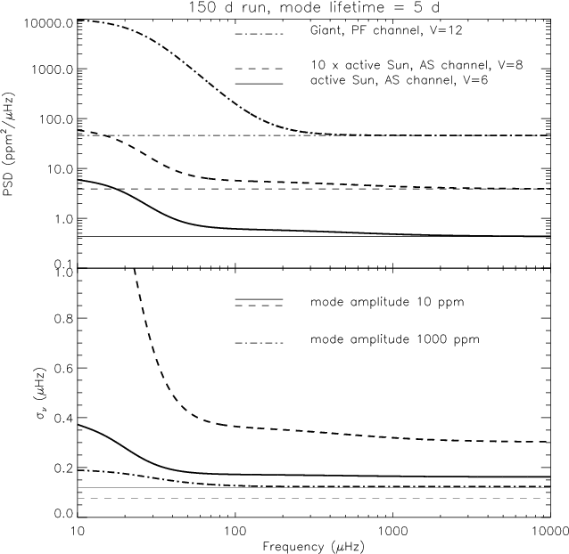 |
Figure 1:
Top panel: typical background power spectrum density
|
| Open with DEXTER | |
3 Analysis of theoretical oscillation spectra
We first generate a coarse grid of equilibrium stellar models with various values of mass (
![]() ,
,
![]() ), luminosity (
), luminosity (
![]() ,
,
![]() )
and effective temperature (
)
and effective temperature (
![]() ,
,
![]() ).
A refined grid is then generated around the stellar parameters which predict
close pulsation spectra, according to the results obtained from the coarse grid.
On this refined grid (
).
A refined grid is then generated around the stellar parameters which predict
close pulsation spectra, according to the results obtained from the coarse grid.
On this refined grid (
![]() ,
,
![]() ,
but constant mass because of time computation), we also vary the mixing-length parameter (
,
but constant mass because of time computation), we also vary the mixing-length parameter (
![]() ,
,
![]() ), the metallicity and helium content
), the metallicity and helium content
![]() (
(
![]() ,
,
![]() )
of the equilibrium model. For this preliminary study, the metallicity Z is varied between
)
of the equilibrium model. For this preliminary study, the metallicity Z is varied between
![]() and Z=0.02. In a forthcoming study,
we plan to include a finer grid for the stellar mass and models with over-solar metallicities.
and Z=0.02. In a forthcoming study,
we plan to include a finer grid for the stellar mass and models with over-solar metallicities.
We use two methods for the comparison between pulsation spectra computed from two different sets of stellar parameters:
- the maximum difference of the frequencies
 of the spectra for given values of the radial order n and of the degree l of the mode;
- the maximum difference of the large separation
 or small separation
 (Kjeldsen et al. 2008).
3.1 Effect of the mixing length parameter
 and of the metallicity Z
We examine the effect of the mixing length parameter
![]() on the spectra in the following way: we fix M, L,
on the spectra in the following way: we fix M, L,
![]() ,
,
![]() and Z and compute, for a given mode (n,l), the difference d
and Z and compute, for a given mode (n,l), the difference d![]() between the frequency for a value of
between the frequency for a value of
![]() and the frequency for a reference value of
and the frequency for a reference value of
![]() (in this case
(in this case
![]() ). The results are shown in Fig. 2.
We performed a similar exercise to estimate the effect of the metallicity Z. The results are displayed in Fig. 3 using a reference value for the metallicity
). The results are shown in Fig. 2.
We performed a similar exercise to estimate the effect of the metallicity Z. The results are displayed in Fig. 3 using a reference value for the metallicity
![]() .
Our preliminary tests show that a variation of
.
Our preliminary tests show that a variation of
![]() or of Z, within reasonable values, can yield a variation of the frequency of a given mode of several
or of Z, within reasonable values, can yield a variation of the frequency of a given mode of several ![]() Hz. These effects need to be investigated in a more systematic study, which we plan for a forthcoming work.
Hz. These effects need to be investigated in a more systematic study, which we plan for a forthcoming work.
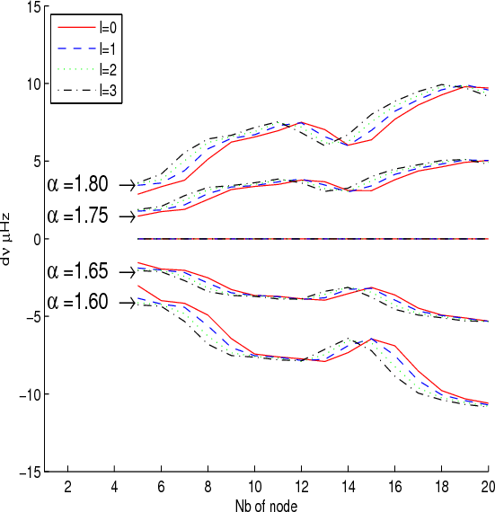 |
Figure 2:
Frequency difference d |
| Open with DEXTER | |
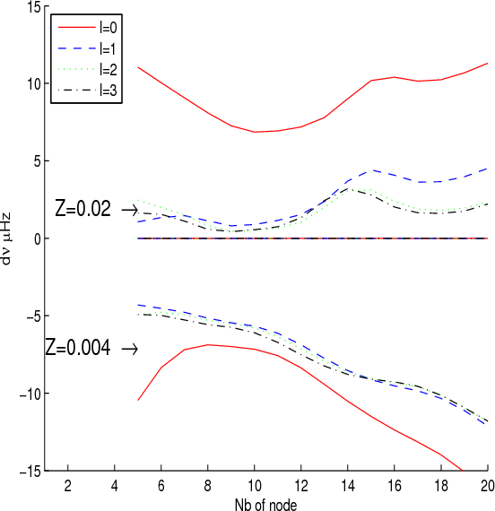 |
Figure 3:
Frequency difference d |
| Open with DEXTER | |
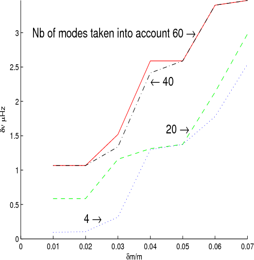 |
Figure 4:
Spectra difference
|
| Open with DEXTER | |
3.2 Comparison between abolute values of frequencies
For a given relative mass difference
![]() ,
the minimum value
,
the minimum value
![]() of
of
![]() is determined in the coarse grid. The value of
is determined in the coarse grid. The value of
![]() depends on the number of considered modes.
We vary this number from 4 (one mode for each value of
depends on the number of considered modes.
We vary this number from 4 (one mode for each value of
![]() )
to 60
(15 modes for each value of
)
to 60
(15 modes for each value of
![]() ). The variation of
). The variation of
![]() with
with
![]() ,
for different numbers of considered modes,
is shown in Fig. 4.
The same procedure is applied for a given luminosity difference
,
for different numbers of considered modes,
is shown in Fig. 4.
The same procedure is applied for a given luminosity difference
![]() or a given radius difference
or a given radius difference
![]() .
The results are shown in
Figs. 5 and 6 respectively.
.
The results are shown in
Figs. 5 and 6 respectively.
As expected, the larger the mass/luminosity/radius difference, the larger the spectra difference.
Similarly, the larger the number of considered modes,
the larger the spectra difference. These trends are the same on the refined grid, but the values for
![]() are much smaller. If we focus on the mass difference, for instance for 40 modes, and
are much smaller. If we focus on the mass difference, for instance for 40 modes, and
![]() ,
,
![]() decreases from 3.4
decreases from 3.4 ![]() Hz on the coarse grid to 0.6
Hz on the coarse grid to 0.6 ![]() Hz on the fine grid, as illustrated in Fig. 7. The effect is similar for the luminosity difference (for 40 modes, and
Hz on the fine grid, as illustrated in Fig. 7. The effect is similar for the luminosity difference (for 40 modes, and
![]() ,
,
![]() decreases from 2.4
decreases from 2.4 ![]() Hz on the coarse grid to 0.5
Hz on the coarse grid to 0.5 ![]() Hz on the fine grid) or the radius difference (for 40 modes, and
Hz on the fine grid) or the radius difference (for 40 modes, and
![]() ,
,
![]() decreases from 6.4
decreases from 6.4 ![]() Hz on the coarse grid to 1.0
Hz on the coarse grid to 1.0 ![]() Hz on the fine grid).
Since we cannot freely refine the grid because of computing time, the values obtained for
Hz on the fine grid).
Since we cannot freely refine the grid because of computing time, the values obtained for
![]() on the refined grid may be overestimated : we cannot exclude that a finer grid gives smaller values of
on the refined grid may be overestimated : we cannot exclude that a finer grid gives smaller values of
![]() .
.
 |
Figure 5:
Spectra difference
|
| Open with DEXTER | |
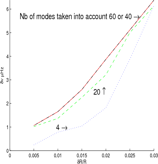 |
Figure 6:
Spectra difference
|
| Open with DEXTER | |
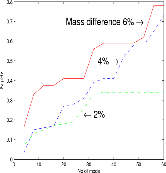 |
Figure 7:
Spectra difference
|
| Open with DEXTER | |
3.3 Large and small separation
Many asteroseismological studies do not directly compare the pulsation frequencies of two stars but rather compare the large and small separations. For this second method, we define the difference
![]() between two spectra as the maximum value of the large separation or of the small separation (the highest value is retained).
The results for the coarse grid, for the mass difference
between two spectra as the maximum value of the large separation or of the small separation (the highest value is retained).
The results for the coarse grid, for the mass difference
![]() with 60 considered modes,
are shown in Fig. 8.
with 60 considered modes,
are shown in Fig. 8.
![]() is about a factor of two lower than
is about a factor of two lower than
![]() .
For the luminosity difference,
.
For the luminosity difference,
![]() is also about a factor of two smaller than
is also about a factor of two smaller than
![]() .
For the radius difference,
.
For the radius difference,
![]() is about a factor of three lower than
is about a factor of three lower than
![]() .
.
As in paragraph 3.2, the same behaviour is found when using the fine grid for a given
![]() ,
,
![]() or
or
![]() .
The results corresponding to a given
.
The results corresponding to a given
![]() are shown in Fig. 9.
are shown in Fig. 9.
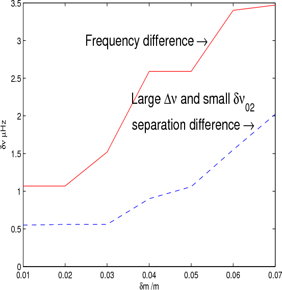 |
Figure 8: Comparison between two methods measuring spectra differences for the coarse grid of models and with 60 considered modes. Red/solid line: frequency difference (Sect. 3.2), blue/dashed line: large or small separation difference (Sect. 3.3). |
| Open with DEXTER | |
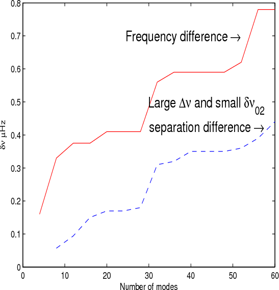 |
Figure 9:
Comparison between two methods measuring spectra differences
for the fine grid of models and for
|
| Open with DEXTER | |
We also examined a third method, where the difference
![]() between two spectra is defined as the difference between the mean large separation or the mean small separation (the highest value is retained). We did not find this method
relevant in the present context (
between two spectra is defined as the difference between the mean large separation or the mean small separation (the highest value is retained). We did not find this method
relevant in the present context (
![]() is found to be negligible for small values of
is found to be negligible for small values of
![]() ,
,
![]() or
or
![]() in the grids studied).
in the grids studied).
4 Discussion and conclusion
The results obtained in Sect. 3 enable us to derive the accuracy of the stellar parameters mass M, luminosity L and radius R determined from asteroseismological data. The accuracy for one parameter is obtained letting all the other parameters remain free. According to Sect. 2.3, we adopt the values of 0.2 ![]() Hz and 0.3
Hz and 0.3 ![]() Hz
respectively for the precision of frequency determination based on the CoRoT performances. The smaller value is for a red giant in the PF channel and the larger value corresponds to the accuracy obtained for a Sun-like star in the AS channel
(see Fig. 1).
Hz
respectively for the precision of frequency determination based on the CoRoT performances. The smaller value is for a red giant in the PF channel and the larger value corresponds to the accuracy obtained for a Sun-like star in the AS channel
(see Fig. 1).
The results are given in Tables 2-4 for an accuracy of the frequency determination of 0.2 ![]() Hz, and in Tables 5-7 for an accuracy of the frequency determination of 0.3
Hz, and in Tables 5-7 for an accuracy of the frequency determination of 0.3 ![]() Hz.
The most stringent constraint is provided by the method using
Hz.
The most stringent constraint is provided by the method using
![]() .
For Sun-like stars as observed in the AS channel, our analysis suggests for instance
an uncertainty for the mass as large as 5% if only 20 modes are
considered
(for the closest models, effective temperatures are compatible within 60K, and radii and luminosities differ by
.
For Sun-like stars as observed in the AS channel, our analysis suggests for instance
an uncertainty for the mass as large as 5% if only 20 modes are
considered
(for the closest models, effective temperatures are compatible within 60K, and radii and luminosities differ by ![]() 2%).
With the method based on
2%).
With the method based on
![]() ,
an uncertainty of 5% for the mass remains for up to 50 considered modes
(for the closest models, effective temperatures are compatible within 60 K, radii differ
by 3% and luminosities are equal).
,
an uncertainty of 5% for the mass remains for up to 50 considered modes
(for the closest models, effective temperatures are compatible within 60 K, radii differ
by 3% and luminosities are equal).
Table 2:
Accuracy
![]() on mass determination, for a frequency accuracy of 0.2
on mass determination, for a frequency accuracy of 0.2 ![]() Hz, obtained from different methods of evaluating spectra difference and for different values of considered modes.
Hz, obtained from different methods of evaluating spectra difference and for different values of considered modes.
Table 3:
Accuracy
![]() on luminosity determination, for a frequency accuracy of 0.2
on luminosity determination, for a frequency accuracy of 0.2 ![]() Hz, obtained from different methods of evaluating spectra difference and for different values of considered modes.
Hz, obtained from different methods of evaluating spectra difference and for different values of considered modes.
Table 4:
Accuracy
![]() on radius determination, for a frequency accuracy of 0.2
on radius determination, for a frequency accuracy of 0.2 ![]() Hz, obtained from different methods of evaluating spectra difference and for different values of considered modes.
Hz, obtained from different methods of evaluating spectra difference and for different values of considered modes.
Table 5:
Same as Table 2 for a frequency accuracy of 0.3 ![]() Hz.
Hz.
Table 6:
Same as Table 3 for a frequency accuracy of 0.3 ![]() Hz.
Hz.
Table 7:
Same as Table 4 for a frequency accuracy of
0.3
Our work is a first step toward a more systematic study, as
it only takes into account variations in
the basic input physics of stellar models such as the mixing length
parameter, the helium abundance and to a certain extent the metallicity.
A more systematic analysis should also explore the
effects of different convection models, of core
overshooting and of rotation. These uncertainties in current stellar evolution
theory will certainly
increase the degeneracy of the pulsation spectra (i.e. the limit on the mass, luminosity or radius
mentioned above may be significantly larger).
Moreover, we have not explored the effect of uncertainties in the stability
analysis calculation, such as the sensitivity to boundary conditions.
The large and small separationsare expected to be less sensitive than absolute frequencies to boundary conditions used in the computation.
Obviously, much additional works need to be done.
Our work, however, provides an idea of the level of accuracy
required by asteroseismological studies in order to improve
exoplanet-host star
parameters, crucial information for future projects such as PLATO.
![]() Hz.
Hz.
C.M.-M. and I.B. acknowledge support from Agence Nationale de la Recherche
under the ANR project number NT05-3 42319.
References
All Tables
Table 1:
Parameters of the background models used. The photon noise level d is given in ppm
![]() ,
while the background amplitudes ai are given in ppm
,
while the background amplitudes ai are given in ppm![]() Hz, and the time-scales bi in 106 s. Three components were used for the Sun-like cases but 2 only for the red giant case.
Hz, and the time-scales bi in 106 s. Three components were used for the Sun-like cases but 2 only for the red giant case.
Table 2:
Accuracy
![]() on mass determination, for a frequency accuracy of 0.2
on mass determination, for a frequency accuracy of 0.2 ![]() Hz, obtained from different methods of evaluating spectra difference and for different values of considered modes.
Hz, obtained from different methods of evaluating spectra difference and for different values of considered modes.
Table 3:
Accuracy
![]() on luminosity determination, for a frequency accuracy of 0.2
on luminosity determination, for a frequency accuracy of 0.2 ![]() Hz, obtained from different methods of evaluating spectra difference and for different values of considered modes.
Hz, obtained from different methods of evaluating spectra difference and for different values of considered modes.
Table 4:
Accuracy
![]() on radius determination, for a frequency accuracy of 0.2
on radius determination, for a frequency accuracy of 0.2 ![]() Hz, obtained from different methods of evaluating spectra difference and for different values of considered modes.
Hz, obtained from different methods of evaluating spectra difference and for different values of considered modes.
Table 5:
Same as Table 2 for a frequency accuracy of 0.3 ![]() Hz.
Hz.
Table 6:
Same as Table 3 for a frequency accuracy of 0.3 ![]() Hz.
Hz.
Table 7:
Same as Table 4 for a frequency accuracy of
0.3 ![]() Hz.
Hz.
All Figures
| |
Figure 1:
Top panel: typical background power spectrum density
|
| Open with DEXTER | |
| In the text | |
| |
Figure 2:
Frequency difference d |
| Open with DEXTER | |
| In the text | |
| |
Figure 3:
Frequency difference d |
| Open with DEXTER | |
| In the text | |
| |
Figure 4:
Spectra difference
|
| Open with DEXTER | |
| In the text | |
| |
Figure 5:
Spectra difference
|
| Open with DEXTER | |
| In the text | |
| |
Figure 6:
Spectra difference
|
| Open with DEXTER | |
| In the text | |
| |
Figure 7:
Spectra difference
|
| Open with DEXTER | |
| In the text | |
| |
Figure 8: Comparison between two methods measuring spectra differences for the coarse grid of models and with 60 considered modes. Red/solid line: frequency difference (Sect. 3.2), blue/dashed line: large or small separation difference (Sect. 3.3). |
| Open with DEXTER | |
| In the text | |
| |
Figure 9:
Comparison between two methods measuring spectra differences
for the fine grid of models and for
|
| Open with DEXTER | |
| In the text | |
Copyright ESO 2009
Current usage metrics show cumulative count of Article Views (full-text article views including HTML views, PDF and ePub downloads, according to the available data) and Abstracts Views on Vision4Press platform.
Data correspond to usage on the plateform after 2015. The current usage metrics is available 48-96 hours after online publication and is updated daily on week days.
Initial download of the metrics may take a while.