| Issue |
A&A
Volume 506, Number 1, October IV 2009
The CoRoT space mission: early results
|
|
|---|---|---|
| Page(s) | 15 - 32 | |
| Section | Stellar structure and evolution | |
| DOI | https://doi.org/10.1051/0004-6361/200911657 | |
| Published online | 03 September 2009 | |
The CoRoT space mission: early results
The solar-like oscillations of HD 49933: a Bayesian approach![[*]](/icons/foot_motif.png) ,
,
O. Benomar - T. Appourchaux - F. Baudin
Institut d'Astrophysique Spatiale, CNRS/Université Paris XI, Bâtiment 121, 91405 Orsay Cedex, France
Received 13 January 2009 / Accepted 27 August 2009
Abstract
Context. Asteroseismology has entered a new era with the availability of continuous observations from space-borne missions such as MOST, CoRoT and Kepler. However, the low amplitude and the complexity of the observed spectrum make the exploitation of these data sets difficult.
Aims. The use of robust methods to estimate the parameters of stellar oscillation eigenmodes is necessary to fully exploit these new data sets. These parameters include in particular the frequency, the width and the energy of the eigenmodes, all being required for a seismic interpretation of the stellar internal structure or excitation of the eigenmodes.
Methods. A Bayesian approach, coupled with a Markov chain Monte Carlo (MCMC) algorithm, is presented. Such a method allows the use of a priori knowledge to improve the parameter estimation. It also provides complete information on the probability distribution of the fitted parameters. The method is tested on simulated time series and then applied to CoRoT observations of HD 49933.
Results. The simulated time series allow the validation of the method for conditions similar to those of the observations in terms of spectral complexity and signal-to-noise ratio. However, a very important problem in the analysis of the HD 49933 mode spectrum is the l degree identification of the modes. The degree identification has little impact on the large frequency separation, rotational splitting, energy and width estimation, whereas individual frequencies and the star inclination angle evaluation are strongly affected. From a statistical point of view, we provide a quantitative ranking of the four models considered. The most probable model includes only modes of degree 0 and 1. Two other models include modes with degree up to 2 and have a non negligible level of significance. The last model includes modes of degree 0 and 1 but has an alternate degree identification and can be definitively rejected. In conclusion, the significance of the resulting probabilities is not sufficient to draw a definite conclusion.
Key words: methods: statistical - methods: observational - stars: oscillations
1 Introduction
The advent of space-borne instruments promises a great harvest of seismic data from stars, with the launch of MOST (2003), CoRoT (2006) and Kepler (2009). Our knowledge of internal stellar structure will certainly be revised and extended in the coming years.
Asteroseismology is based essentially on the analysis of the oscillatory variation of an observable (intensity or surface velocity) of the star. Resonant modes appear as peaks in the Fourier spectrum of this observable, characterized by their frequency, height and width, on which further seismic interpretation is based. For stochastically excited oscillations (also called solar-like oscillations), the mode parameters are determined by maximizing the likelihood of a model spectrum with respect to the observed power spectrum (Toutain & Fröhlich 1992; Appourchaux et al. 1998; Anderson et al. 1990). This is a complex and sensitive process, subject to spurious estimates if, for example, the signal-to-noise ratio is low, which could introduce local maxima of the likelihood leading to wrong estimates. If one aims at an automatic analysis of a large quantity of data, expected for present and future space missions, more robust methods are necessary.
A promising way to accomplish this is to use a Bayesian analysis. The Bayesian approach is well suited to extract as much information as possible from a given data set by including a priori knowledge from other data sets or theoretical assumptions. This approach determines the so-called a posteriori probability distribution of a given parameter from a combination of the likelihood of a model with respect to the observation with an a priori probability distribution for this parameter, which reflects some supposed knowledge of this parameter. Moreover, based on these posterior probabilities, the Bayesian analysis allows the comparison of different models to be fitted to the data and provides a quantitative means to decide which model is the most probable. Recently, more and more astronomers have begun to use this approach in different domains (e.g. Gregory 2005a; Parkinson et al. 2006; Brewer et al. 2007; Carrier et al. 2007).
The efficiency of this approach is enhanced if it utilizes all of the information contained in the posterior probability distribution function (pdf), and not only on the determination of its maximum. In some cases, the probability distribution of a parameter will not be as simple as a Gaussian or any other mono-modal function but may consist of multi-modal functions. When dealing with a small number of parameters (of the order of a dozen), analytical or numerical approximations are well suited and allow the construction of the probability distribution of the parameters. This becomes problematic when the number of parameters is large (several tens). In this case, it is preferable to use stochastic simulations and especially Markov chains based on Monte Carlo simulations (hereafter MCMC) which provide a solution to the difficult problem of the sampling of a space with a large number of dimensions. An MCMC can be considered as a chain of random walks in the parameter space in which each step depends only on the immediate previous position: this is a weak memory process. An MCMC is able to sample, for example, a probability density function (pdf) whatever the complexity of its analytical expression. Moreover, compared to most analytical or numerical strategies (such as gradient methods used to find the maximum of a function), they are insensitive to the initial starting point in the parameter space. An MCMC is able to explore and sample all of the regions of the parameter space where the pdf is significant. Consequently, if multiple maxima exist, an MCMC based algorithm will sample all of them and not only one or a few of them. More technical details about MCMC are given in the Appendix.
In Sect. 2, we consider the issues related to solar-like stars and the analysis of their power spectra. In Sect. 3, we present technical aspects regarding the Bayesian mathematics. Section 4 presents our results with simulated data illustrating the efficiency of the Bayesian approach coupled to the MCMC sampling technique. Section 5 presents our results on a star observed by CoRoT (HD 49933). This is a difficult case, and we discuss our results and earlier ones. Section 6 summarizes the results and perspectives.
2 Solar-like physical considerations
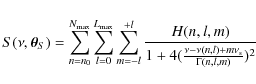
A star acts as a resonant cavity and different modes can be excited. These resonances appear as peaks in the Fourier spectrum of, for example, stellar photometric variations. We deal here with solar-like pulsators, or stars showing many acoustic modes (p modes) that are stochastically excited. In the solar case, the source of excitation is the convection of the upper layers of the star. To a first approximation, each mode can be characterized by a lifetime, a frequency and an energy, and described as a Lorentzian profile in the power spectrum. Hence, the stellar oscillation spectrum can be expressed as:
 |
(1) |
where
with
The stellar signal also includes a background component. In the solar case, this background can be described by a sum of Lorentzian-like profiles, first introduced by Harvey (1985),
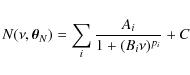
where
Finally, writing the entire parameter set
![]() ,
a representative model of the solar-like stellar spectrum is:
,
a representative model of the solar-like stellar spectrum is:
| (4) |
3 Bayesian approach
3.1 Bayesian formalism
In the case of photometric measurements, the noise affecting the stellar intensity variations obeys Gaussian statistics (Appourchaux et al. 1998). Hence, the imaginary and real part of the Fourier spectrum are also Gaussian. Thus, the noise power spectrum follows a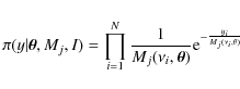
where N is the number of frequency samples
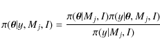
From Bayes theorem, we can define the posterior pdf:
 |
(6) |
where
 |
(7) |
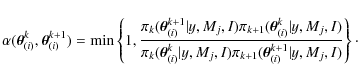
3.2 Model comparison
In the Bayesian formalism, it is also possible to compare different models by using Bayes' rule to define the posterior probability
P(Mj|y,I) of a model Mj being consistent with the data y,
P(y|Mj,I) represents the global likelihood, P(Mj|I) the prior of the model and P(y|I) a normalization constant for the whole model space. In the present comparisons, we attribute the same prior probability to each model. Thus, comparing models Mj and Mk in a Bayesian approach relies on the ratio of the global likelihoods only. OMj,Mk is called the odds ratio,
This is different from the MLE approach where we compare maximum likelihoods. The model Mj is more favored by the data than Mk if OMj,Mk>1. In practice, when 1<OMj,Mk<3, Mj is barely supported but this support becomes substantial for OMj,Mk>3. OMj,Mk=3 corresponds to 75% probability. We can also calculate the relative probability of a model Mj over the discrete explored model space of size
The calculation of the global likelihood requires a process known as marginalization. It consists of removing the parameter dependence by integration over all of the variable parameters of the conditional likelihood weighted by the prior pdf of the considered model,
Marginalization is difficult to achieve analytically in most cases because of the complexity of the function to be integrated. With the expression of the likelihood of Eq. (5), it is not possible and only a numerical evaluation is feasible. If the size of the parameter space is small, we can evaluate the integral by a simple Monte-Carlo approach, but this becomes very difficult for a large (several tens) number of parameters. An alternative approach consists of sampling the parameter space by using a MCMC algorithm. MCMC simulations have the advantage of providing an integral evaluation and thus marginalization capabilities from the sampling of the function to be integrated. This makes the global likelihood computation easy, even for complex expressions such as
3.3 Bayesian priors for solar-like pulsators
We can now apply the Bayesian approach using our knowledge of solar-like stars. We will restrict ourselves to spatially unresolved photometric stellar observations: in the best case, the mode visibility is too low to distinguish modes with a degree l higher than 3 in the power spectrum.
Referring to Eq. (2) we see that the frequency of the l=2 and l=3 modes can be written relative to the l=0 and l=1 modes, respectively:
These differences are called the small separations. Each l=0 mode has an l=2 companion. Similarly, each l=1 mode has an l=3 neighbor. In the present case, as was already noted by Appourchaux et al. (2008), Benomar (2008) and Gruberbauer et al. (2009), it is clear that the signal-to-noise ratio is low, even for the l=0 and l=1 modes. These modes are supposed to have the highest signal-to-noise ratio and the l=3 mode is known to have a very low relative height (
In an observed power spectrum, we can have two different l degree identifications (hereafter, models ![]() and
and ![]() )
for a given peak in the spectrum: one can choose
to consider that this peak is made of a pair of l=0,2 modes or just made of an l=1 mode, as these two structures alternate in the spectrum.
If the l=2 modes appear clearly in the spectrum, there is no doubt about the identification as it makes the peak wider. But if this is not the case (e.g. low signal-to-noise condition, say H/N < 10 for the l=0 modes, or l=0 and l=2 mode overlap), the identification becomes difficult. In the Bayesian context, the mode identification can be achieved using the odds ratio (Eq. (10)). In this case, the equation can be rewritten as
)
for a given peak in the spectrum: one can choose
to consider that this peak is made of a pair of l=0,2 modes or just made of an l=1 mode, as these two structures alternate in the spectrum.
If the l=2 modes appear clearly in the spectrum, there is no doubt about the identification as it makes the peak wider. But if this is not the case (e.g. low signal-to-noise condition, say H/N < 10 for the l=0 modes, or l=0 and l=2 mode overlap), the identification becomes difficult. In the Bayesian context, the mode identification can be achieved using the odds ratio (Eq. (10)). In this case, the equation can be rewritten as
 |
(13) |
By convention, we will denote by
To evaluate the two hypotheses, we propose to use a prior for the frequencies of the l=0 and l=1 modes of order n between
![]() and
and
![]() :
:
![$\displaystyle \times\sum_{n=n_{\rm min}}^{n_{\rm max}}{\left[ {\rm e}^{-\frac{(\nu-\nu(n,0))^2}{2\sigma^2}}+{\rm e}^{-\frac{(\nu-\nu(n,1))^2}{2\sigma^2}}\right]}$](/articles/aa/full_html/2009/40/aa11657-09/img48.png)
where
The priors for l=2 mode frequencies are described by a Gaussian prior to the small separation,
where
Here, we define and use as a parameter the mode height of a mode relative to the height of the radial mode l=0:
Vl=1=Hl=1/Hl=0 and
Vl=2=Hl=2/Hl=0. In the case of long duration observations, the mode height ratios are essentially constrained by a geometrical visibility factor (Toutain & Gouttebroze 1993) and are thus independent of ![]() .
For the inputs to our simulations (Sect. 4), we used the solar relative height ratio for unresolved photometric observations:
Vl=1=1.5 and
Vl=2=0.5. However, for the analysis, the relative heights are not fixed, unlike previous approaches (Benomar 2008; Appourchaux et al. 2008).
.
For the inputs to our simulations (Sect. 4), we used the solar relative height ratio for unresolved photometric observations:
Vl=1=1.5 and
Vl=2=0.5. However, for the analysis, the relative heights are not fixed, unlike previous approaches (Benomar 2008; Appourchaux et al. 2008).
The Jeffrey prior (
![]() )
can be appropriate in the case of
scale parameters (e.g. parameter such as f(x)=ax, where a is a ``scale'' factor), which is the case of
the height and the width of the modes. Such a prior is non-informative and uniform in the logarithmic domain. Jeffrey (1961) justified the choice of this kind of prior as they are invariant under parameter transformation. However, this prior is improper (integration over x yielding an undefined result) and it is common to use a truncated version of this prior:
)
can be appropriate in the case of
scale parameters (e.g. parameter such as f(x)=ax, where a is a ``scale'' factor), which is the case of
the height and the width of the modes. Such a prior is non-informative and uniform in the logarithmic domain. Jeffrey (1961) justified the choice of this kind of prior as they are invariant under parameter transformation. However, this prior is improper (integration over x yielding an undefined result) and it is common to use a truncated version of this prior:
![]() where
where
![]() is the normalization constant.
is the normalization constant.
![]() and
and
![]() are upper and lower bounds such that if
are upper and lower bounds such that if
![]() or
or
![]() then
then
![]() .
Thus, the probability density is proper (integral over x is finite). Unfortunately the truncation, although it renders the probability density proper, may not follow the prescription of Jeffrey (1961) of invariance. This should be borne in mind.
.
Thus, the probability density is proper (integral over x is finite). Unfortunately the truncation, although it renders the probability density proper, may not follow the prescription of Jeffrey (1961) of invariance. This should be borne in mind.
Another non-informative prior is the uniform prior (
![]() if
if
![]() ,
else
,
else
![]() ). It is recommended by Jeffrey when dealing with ``location'' parameters (parameters such as f(x)=x+a), which is the case of the mode frequencies.
We compared the effect of these two priors applied to the height and width on the model probability in the case of scenario 4 and 5 (see the next section for more information about the explored
scenarios). In these scenarios, we compare two models
). It is recommended by Jeffrey when dealing with ``location'' parameters (parameters such as f(x)=x+a), which is the case of the mode frequencies.
We compared the effect of these two priors applied to the height and width on the model probability in the case of scenario 4 and 5 (see the next section for more information about the explored
scenarios). In these scenarios, we compare two models
![]() and
and
![]() .
We note that using a Jeffrey prior for the scale parameters leads to an increase in the contrast of the relative model probability (about 0.2-0.4 dex or 10%-20% in probability).
However, this variation can also be attributed to the probability estimation method itself (i.e. numerical calculation in Sect. A.3). The estimate of the uncertainty of the probability calculated by MCMC is still an open issue: for the conditions described throughout this article, two successive and independent algorithm executions on the same data set provide probability results with a log probability difference of the order of 0.2 dex.
.
We note that using a Jeffrey prior for the scale parameters leads to an increase in the contrast of the relative model probability (about 0.2-0.4 dex or 10%-20% in probability).
However, this variation can also be attributed to the probability estimation method itself (i.e. numerical calculation in Sect. A.3). The estimate of the uncertainty of the probability calculated by MCMC is still an open issue: for the conditions described throughout this article, two successive and independent algorithm executions on the same data set provide probability results with a log probability difference of the order of 0.2 dex.
The relative heights H(n,l,m) of the split components of nonradial modes depend on the angle between the line of sight of the observer and the rotation axis of the star (see for ex. Gizon & Solanki 2003). Knowing that, we can define the heights of these components as a function of the angle. Depending on the available information, an angle prior can be set or not; here, in the case of the analysis of the simulated spectra (Sect. 4) or the real data (Sect. 5), a uniform prior over the range 0
![]() is set.
is set.
Regarding the background, we adopted a two-step strategy:
- 1.
- we fit the power spectrum over a large frequency range (in the case of HD 49933, 0-5000
 after removing the spacecraft orbital peaks) with 3 Lorentzian shaped components and a white noise (Eq. (3)) plus a Gaussian profile (characterized by its height A0, its central frequency
 ,
and its width
,
and its width
 )
to globally describe the modes. The slope of the Lorentzian profiles are assumed to be equal (
p1=p2=p3=p). At this point we have 11 free parameters;
)
to globally describe the modes. The slope of the Lorentzian profiles are assumed to be equal (
p1=p2=p3=p). At this point we have 11 free parameters;
- 2.
- we verify that the Lorentzian describing the granulation background is effectively the dominant one in the p mode frequency range. Then, we neglect the two other components and we use the posterior results to constrain the background in the mode range (1210-4000
 )
with Gaussian priors.
)
with Gaussian priors.
4 Illustrative simulations
4.1 Simulation conditions
![\begin{figure}
\par\includegraphics[angle=90,width=7cm,clip]{11657_E.ps}\par\vspace*{2mm}
\includegraphics[angle=90,width=7cm,clip]{11657_F.ps}
\end{figure}](/articles/aa/full_html/2009/40/aa11657-09/img69.png) |
Figure 1: a) Smoothed power spectrum of HD 49933, showing activity (dot-dashed line) and granulation (solid line) backgrounds and stellar modes.The modes are first modeled by a Gaussian (solid blue curve). b) Mode frequency range with frequency priors (l=0: red dash line; l=1: green dot line) for the mode identification A. |
| Open with DEXTER | |
In order to check the reliability (in particular for the mode identification) of the method presented here, simulated spectra were simulated with different inputs in terms of noise level and stellar parameters, yielding an ensemble of six test scenarios. All of them correspond to the mode identification A used for the analysis of HD 49933 (see Sect. 5).
Most of the synthetic spectra (scenarios 1 to 5) contain the 3 first degrees (l=0 to l=2) for 8 radial orders. The relative heights Vl=1 and Vl=2 are fixed at the solar values. The background is composed of a Lorentzian profile plus white noise. The frequency resolution is set to 0.2
![]() which corresponds to an observation duration of about 58 days. Different scenarios were tested by changing the height, the width, the rotational splitting and the small separation
which corresponds to an observation duration of about 58 days. Different scenarios were tested by changing the height, the width, the rotational splitting and the small separation
![]() .
The frequencies follow an asymptotic law, with
.
The frequencies follow an asymptotic law, with
![]() Hz. The inclination angle is set to 40
Hz. The inclination angle is set to 40![]() .
Scenario 6 considers the case of a power spectrum with only 2 degrees (l=0 and l=1). For a summary of the input spectrum parameters, see Table 1.
.
Scenario 6 considers the case of a power spectrum with only 2 degrees (l=0 and l=1). For a summary of the input spectrum parameters, see Table 1.
We explored four kinds of scenarios:
- 1.
- relatively high H/N ratio (>30), distant neighboring l=2 and l=0 modes and small rotational splitting (
 ). These conditions reduce the mode multiplet superposition (scenario 1);
- 2.
- identical to the previous scenario but for a relatively low H/N ratio, around 4 (scenario 2);
- 3.
- intermediate H/N ratio (around 3 to 12) with a
 ,
leading to a superposition of the split components of the l=2 and the l=0 modes. The widths are chosen particularly large to increase the difficulty of separating the neighboring modes (scenario 3 to 5);
,
leading to a superposition of the split components of the l=2 and the l=0 modes. The widths are chosen particularly large to increase the difficulty of separating the neighboring modes (scenario 3 to 5);
- 4.
- scenario 6 is designed to test the algorithm in the case of an overinterpretation of the spectrum: only l=0 and l=1 modes are included in the simulated spectrum but mode indentifications including l=2 modes are tested (thus, four models are tested: the two possible mode identifications A and B, with and without l=2).
Table 1: Input parameters used for the simulated spectra.
Table 2:
Priors used for the analysis of the simulated spectra for the inclination angle i, the rotational splitting
![]() ,
the large separation
,
the large separation ![]() (Eq. (2)) and the small separation
(Eq. (2)) and the small separation
![]() (Eq. (15)).
(Eq. (15)).
4.2 Simulation results
Table 3:
Top: model odds ratio
![]() for scenario 1 to 5 (which include l=2 modes). Bottom: odds ratio for scenario 6, comparing 4 models (identifications A and B, with or without l=2).
for scenario 1 to 5 (which include l=2 modes). Bottom: odds ratio for scenario 6, comparing 4 models (identifications A and B, with or without l=2).
For each scenario, we acquire 1 000 000 samples after a burn-in phase, during which the MCMC algorithm progresses towards the values of interest (i.e. with significant probabilities) while the acceptance rate is adjusted.
For scenarios 1 to 3, the mode identification is correct with a confidence of more than 99.99%. The odds ratio is systematically in favor of the correct identification even for low signal-to-noise conditions. We remark that the l=0-2 modes overlap and the large width ![]() strongly decrease the odds ratio (see Table 3). For very large width, the odds ratio becomes ambiguous (scenario 5) and we are not able to decide which model is the most realistic. In scenario 6, the priors on the small separation
strongly decrease the odds ratio (see Table 3). For very large width, the odds ratio becomes ambiguous (scenario 5) and we are not able to decide which model is the most realistic. In scenario 6, the priors on the small separation
![]() act as expected by penalizing the more complex models. The most probable model is the correct one but with a confidence of only about
act as expected by penalizing the more complex models. The most probable model is the correct one but with a confidence of only about ![]() .
.
| |
Figure 2:
l=2 mode relative height from simulation (scenario 3) for the correct identification a) and for the wrong identification b). In the correct identification, due to the l=0 and l=2 mode superposition, the relative height H2/H0 is underestimated by 30%. In the wrong identification, the distribution of the height follows the |
| Open with DEXTER | |
The observation of the frequency posterior distributions shows that an error on the model choice easily leads to multimodal pdf. The relative height Vl=2 is also strongly affected as it follows a ![]() distribution with a 2 d.o.f. statistics in the wrong identification case, similarly to the noise distribution. In scenario 3, the retrieved mean median value of the small separation
distribution with a 2 d.o.f. statistics in the wrong identification case, similarly to the noise distribution. In scenario 3, the retrieved mean median value of the small separation
![]() is
is
![]() Hz, to be compared to the input value of
Hz, to be compared to the input value of ![]() Hz. The prior and/or the l=0, l=2 mode overlap seems to shift the estimation by about 1
Hz. The prior and/or the l=0, l=2 mode overlap seems to shift the estimation by about 1
![]() .
However, this offset remains smaller than the 2
.
However, this offset remains smaller than the 2![]() interval.
interval.
![\begin{figure}
{\vbox{
\hbox{
\epsfig{figure=11657_I.ps,width=4.0cm,angle=90}\ep...
...ps,width=4.0cm,angle=90}\hfill
\hspace{3mm}
\parbox[b]{50mm}{
}
}}}
\end{figure}](/articles/aa/full_html/2009/40/aa11657-09/img100.png) |
Figure 3:
HD 49933 typical frequency, height, width and amplitude pdf (here for model
|
| Open with DEXTER | |
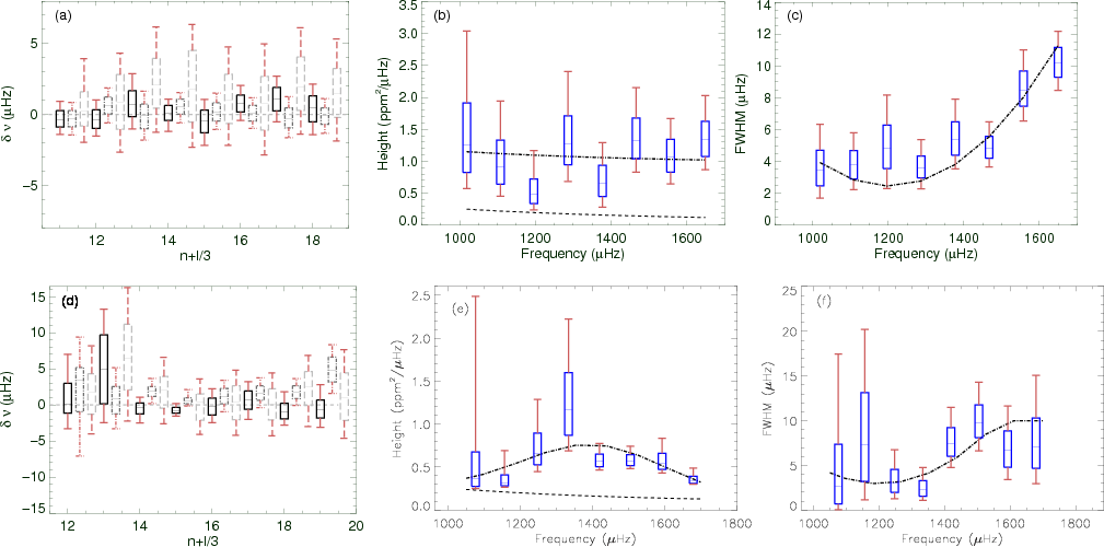 |
Figure 4:
Comparison of the output and input values for simulated spectra, for scenario 3 ( a), b), c)) and for scenario 4 ( d), e), f)). The box represent the 68.3% confidence interval (1 |
| Open with DEXTER | |
The non-Gaussian shape of the pdf obtained in some cases (especially for heights and widths), and the multi-modal shape of the pdf, raise the problem of the estimator choice and of the error bar definition. In statistical terms and in terms of parameter estimation, it is interesting to refer to the median which is considered to be a good alternative to the Maximum a posteriori (MAP) inference (Gregory 2005b). The maximum of a pdf is a poor estimator as it does not provide global information about the pdf. It is also very difficult to evaluate the maximum of a pdf as the sampling may not be sufficient. To illustrate the inadequacy of the pdf maximum as a good estimator, we can consider the example of the ![]() noise pdf. It is a decreasing exponential and the maximum will give a zero value whatever the noise level. Moreover, the width and mode height are known to not be distributed as a Gaussian.
noise pdf. It is a decreasing exponential and the maximum will give a zero value whatever the noise level. Moreover, the width and mode height are known to not be distributed as a Gaussian.
Generally, the mode parameter pdfs are supposed has being Gaussian and as a consequence, the error bars are symmetrical and given at ![]() 1
1![]() which corresponds to a 68.3% confidence interval. As we often deal with more complex pdfs, we must provide either the pdf or multiple confidence indicators to summarize the function and describe how spread it is. To fully describe the variety of the pdfs, we decided to provide the confidence intervals at 68.3% and 95.5%, (corresponding to 1 and 2
which corresponds to a 68.3% confidence interval. As we often deal with more complex pdfs, we must provide either the pdf or multiple confidence indicators to summarize the function and describe how spread it is. To fully describe the variety of the pdfs, we decided to provide the confidence intervals at 68.3% and 95.5%, (corresponding to 1 and 2![]() ,
respectively, for a Gaussian distribution) centred on the median. The confidence interval determination involves a cumulative probability function calculation. Thus, the tables of results contain 5 values per parameter: the median and asymmetrical
,
respectively, for a Gaussian distribution) centred on the median. The confidence interval determination involves a cumulative probability function calculation. Thus, the tables of results contain 5 values per parameter: the median and asymmetrical ![]() and
and ![]() equivalent confidence ranges.
equivalent confidence ranges.
Following these definitions, most of the inputs used to build the different synthetic spectra are within a 95.5% confidence interval of the estimated values resulting from the analysis of these spectra. All of them exceed 99.7% (3![]() equivalent) confidence. The estimates of height and width are poor even in good signal-to-noise cases (see Fig. 4), whereas frequencies are very well determined, with a typical error tending to the spectrum resolution in the most favorable cases (scenario 1). A systematic underestimation (
equivalent) confidence. The estimates of height and width are poor even in good signal-to-noise cases (see Fig. 4), whereas frequencies are very well determined, with a typical error tending to the spectrum resolution in the most favorable cases (scenario 1). A systematic underestimation (![]()
![]() )
of the relative height H2/H0 occurs in the case of l=0 and l=2 mode superposition.
)
of the relative height H2/H0 occurs in the case of l=0 and l=2 mode superposition.
5 The Bayesian analysis of HD 49933
The analysis of HD 49933 (a main sequence F5V star) was carried out using a 60-day time series of CoRoT observations (IRa01). This star has been observed previously from the ground (Mosser et al. 2005) and from space by CoRoT. A first analysis of the latter data has been carried out by Appourchaux et al. (2008) using a simple likelihood maximization (MLE) approach. These data were also studied by Benomar (2008) and Gruberbauer et al. (2009), using a Bayesian approach.
The main characteristics of this star can be summarized as follows: an estimated mass of ![]()
![]() (Mosser et al. 2005), radius
(Mosser et al. 2005), radius
![]() of
of
![]() (Thévenin et al. 2006);
(Thévenin et al. 2006); ![]() estimates by different sources lead to values from
estimates by different sources lead to values from
![]() km s-1 (Mosser et al. 2005) to 10.9 km s-1 (Solano et al. 2005). As reported by Appourchaux et al. (2008), the low frequency power spectrum shows a strong peak at 3.4
km s-1 (Mosser et al. 2005) to 10.9 km s-1 (Solano et al. 2005). As reported by Appourchaux et al. (2008), the low frequency power spectrum shows a strong peak at 3.4
![]() understood as the signature of the rotation period, caused by the
transit of active regions across the surface of HD 49933. Then, from radius and
understood as the signature of the rotation period, caused by the
transit of active regions across the surface of HD 49933. Then, from radius and ![]() estimates, the angle i between the line of sight and the stellar rotation axis appears to be between 22 and 30
estimates, the angle i between the line of sight and the stellar rotation axis appears to be between 22 and 30![]() while the asteroseismic study of Appourchaux et al. (2008) leads to an angle value between 50 and 62
while the asteroseismic study of Appourchaux et al. (2008) leads to an angle value between 50 and 62![]() (for these authors, a possible reason for this discrepancy is the probable superposition of the l=2 and l=0 modes).
(for these authors, a possible reason for this discrepancy is the probable superposition of the l=2 and l=0 modes).
Table 4:
Priors used for HD 49933 data analysis.
![]() is the rotational splitting, i the star inclination angle,
is the rotational splitting, i the star inclination angle,
![]() the small frequency separation,
the small frequency separation, ![]() the large separation. The value of
the large separation. The value of ![]() and D0 depend on the model and set the position of the first prior frequency (see Eq. (2)).
and D0 depend on the model and set the position of the first prior frequency (see Eq. (2)).
Table 5: Model odds ratio and estimated probability for HD 49933 spectrum analysis. The value of the matrix represents the odds ratio.
This information can be used to set some priors. The splitting prior is set by supposing that the rotation signature at 3.4
![]() is representative of the internal stellar rotation. As in the simulation, the standard deviation is fixed at 10% of the expected value. Because of the inconsistency previously described for the angle i, we prefer not to impose a prior on i: we use a uniform prior between 0
is representative of the internal stellar rotation. As in the simulation, the standard deviation is fixed at 10% of the expected value. Because of the inconsistency previously described for the angle i, we prefer not to impose a prior on i: we use a uniform prior between 0![]() and 90
and 90![]() .
As in Benomar (2008), the large separation prior is set to
.
As in Benomar (2008), the large separation prior is set to
![]()
![]() and the small separation
and the small separation
![]() at
at ![]()
![]() using stellar model information. Priors on mode frequencies are Gaussian with a width of 8
using stellar model information. Priors on mode frequencies are Gaussian with a width of 8 ![]() Hz. All of the priors are described in Sect. 3.3 and summarized in Table 4.
Hz. All of the priors are described in Sect. 3.3 and summarized in Table 4.
The power spectrum of the time series is computed once a second order polynomial has been removed from the original time series. This spectrum is normalized such that the total power integrated from zero to twice the Nyquist frequency equals the lightcurve variance. 15 mode profiles were fitted to this spectrum in a frequency interval from 1210 to 4000
![]() .
The pdf estimations are based on 2 000 000 samples (for each Markov chain).
.
The pdf estimations are based on 2 000 000 samples (for each Markov chain).
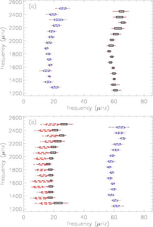 |
Figure 5:
HD 49933 echelle diagram for the model
|
| Open with DEXTER | |
The present work differs from that of Gruberbauer et al. (2009) as they did not take into account the rotational splitting and the inclination angle and assumed a constant mode width whereas we have considered this hypothesis too strong and have included rotation and variable mode widths in our description. As already mentioned, Appourchaux et al. (2008) used a MLE approach. Benomar (2008) used a Bayesian approach but in a less sophisticated manner: for example, the question of the presence of l=2 modes was not tested in the process of mode identification.
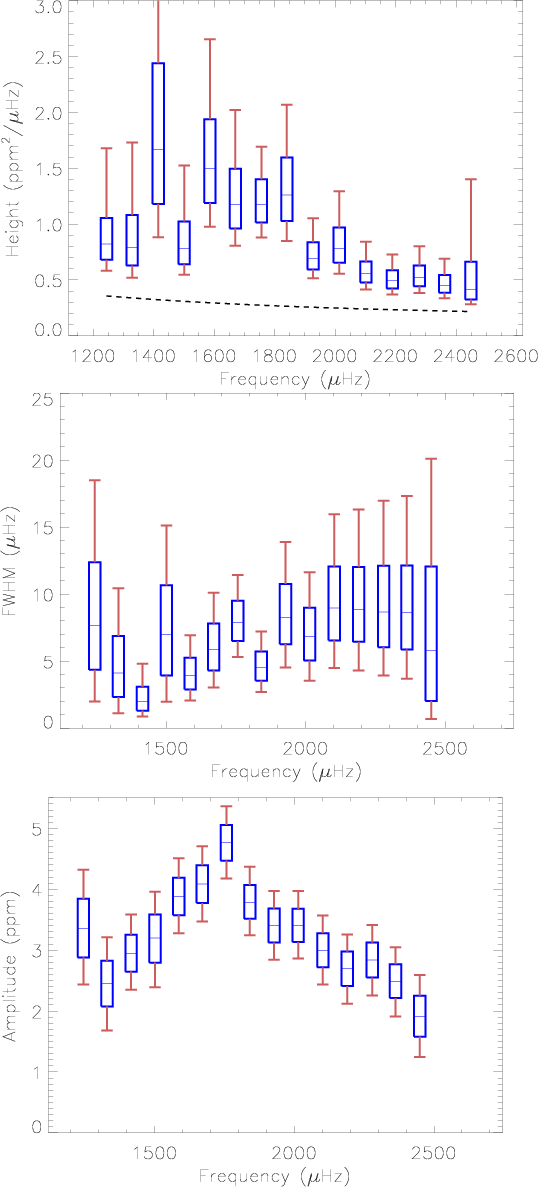 |
Figure 6:
Estimated heights, width and amplitude for model
|
| Open with DEXTER | |
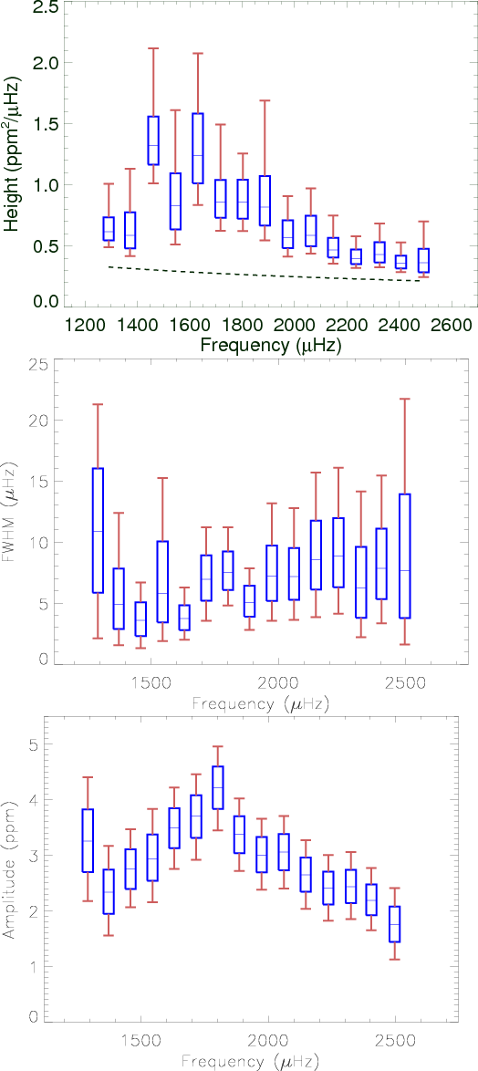 |
Figure 7:
Estimated heights, width and amplitude for model
|
| Open with DEXTER | |
Here, we compared 4 models using Eqs. (9) and (10): the two possible mode identifications and the presence or absence of the l=2 modes. The probabilities obtained are summarized in Table 5. The most probable model (
![]() )
corresponds to the same mode identification as offered by Appourchaux et al. (2008) but it does not include the l=2 modes. While the criteria used by Appourchaux et al. (2008) are based on the comparison of the maximum likelihoods, here we estimate the global probability which we consider more reliable and more conservative. Moreover Appourchaux et al. (2008) did not explore the possibility of the absence of the l=2 modes. Here, the most probable model (
)
corresponds to the same mode identification as offered by Appourchaux et al. (2008) but it does not include the l=2 modes. While the criteria used by Appourchaux et al. (2008) are based on the comparison of the maximum likelihoods, here we estimate the global probability which we consider more reliable and more conservative. Moreover Appourchaux et al. (2008) did not explore the possibility of the absence of the l=2 modes. Here, the most probable model (
![]() )
contains only the l=0 and l=1 modes. Occam's principle, naturally implemented in the Bayesian approach, penalizes the more complex model and thus favors models without l=2 modes. However, adding the l=2 modes to the identification B (comparison between
)
contains only the l=0 and l=1 modes. Occam's principle, naturally implemented in the Bayesian approach, penalizes the more complex model and thus favors models without l=2 modes. However, adding the l=2 modes to the identification B (comparison between
![]() and
and
![]() )
strongly reinforces its credibility, but not sufficiently so to definitely overrule the A identification.
)
strongly reinforces its credibility, but not sufficiently so to definitely overrule the A identification.
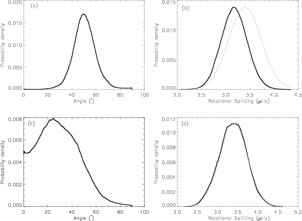 |
Figure 8:
Posterior probability density function for the rotational splitting and the inclination angle of HD 49933 for each possible mode identification including l=2 for model
|
| Open with DEXTER | |
Table 6:
HD 49933 frequencies and height-to-noise posterior estimates for l=0 and l=1 modes for the
![]() model.
model.
A complementary explanation of the difficulty of retrieving the l=2 could be that the background model may not be representative of the real nature of the granulation background. At the current signal-to-noise ratio, a good prior knowledge is critical for mode parameter estimation. The estimated model probability might also be strongly affected by the chosen background model, as this latter can bias the observed heights of the modes. Nevertheless, it is clear that a low value of the small separation combined with large linewidth and splitting introduces crosstalk between the l=0 and l=2 modes, especially for the frequency and height estimation, and renders the l=2 extraction difficult, if not impossible.
Nevertheless, notice that the odds ratio between the two most probable models is lower than 3 (cf. Table 5). Despite having the highest level of confidence, the
![]() model is not strongly supported by the data. We also notice that the inclination angle for the identification B is much closer to the expected value from non seismic observations. It is likely that if we had imposed a prior on this parameter using
model is not strongly supported by the data. We also notice that the inclination angle for the identification B is much closer to the expected value from non seismic observations. It is likely that if we had imposed a prior on this parameter using ![]() and the estimate radius, we would have obtained a stronger probability for the identification B. The only model that can be reasonnably excluded is
and the estimate radius, we would have obtained a stronger probability for the identification B. The only model that can be reasonnably excluded is
![]() .
.
The model choice does not significantly affect the estimation of the mean large separation. Its value is compatible at the ![]() level with Appourchaux et al. (2008) (
level with Appourchaux et al. (2008) (
![]() )
whichever the model chosen here (see Table 9).
)
whichever the model chosen here (see Table 9).
The estimated rotational splitting for the model
![]() is slightly lower than for the model
is slightly lower than for the model
![]() but both are compatible with the results of MLE (Appourchaux et al. 2008). The posterior pdf of the rotational splitting for this latter model is probably dominated by its prior rather than its likelihood (see Fig. 8). This is not surprising, as a low stellar inclination leads to a very low height of the split component of all degrees l except for the m=0 component, making the splitting weakly constraining.
but both are compatible with the results of MLE (Appourchaux et al. 2008). The posterior pdf of the rotational splitting for this latter model is probably dominated by its prior rather than its likelihood (see Fig. 8). This is not surprising, as a low stellar inclination leads to a very low height of the split component of all degrees l except for the m=0 component, making the splitting weakly constraining.
We have also expressed the mode energy pdf by the product
![]() which we summarize in Table 8. Energies are relatively well constrained in comparison with heights and widths. Models without l=2 have slightly higher l=0 mode energy than the models with l=2 as the total observed energy remains constant.
Figures 6 and 7 show the variations versus frequency of the heights, widths and energies for the models
which we summarize in Table 8. Energies are relatively well constrained in comparison with heights and widths. Models without l=2 have slightly higher l=0 mode energy than the models with l=2 as the total observed energy remains constant.
Figures 6 and 7 show the variations versus frequency of the heights, widths and energies for the models
![]() and
and
![]() .
We notice through the error bars that the pdf dispersion is higher than in our simulations for a comparable height-to-noise ratio, especially for the widths. Multiple factors can be the source of these differences. First, our simulations are certainly simpler than reality. Moreover the p mode model and the stellar noise model may
be inappropriate. It is possible for example that the mode widths are poorly determined because of a strong asymmetry of the split components and of their profiles.
Compared to Appourchaux et al. (2008), some differences can be noticed at high frequency for the width. In particular, we find again the plateau beyond 1700
.
We notice through the error bars that the pdf dispersion is higher than in our simulations for a comparable height-to-noise ratio, especially for the widths. Multiple factors can be the source of these differences. First, our simulations are certainly simpler than reality. Moreover the p mode model and the stellar noise model may
be inappropriate. It is possible for example that the mode widths are poorly determined because of a strong asymmetry of the split components and of their profiles.
Compared to Appourchaux et al. (2008), some differences can be noticed at high frequency for the width. In particular, we find again the plateau beyond 1700
![]() for the width but with larger error bars.
for the width but with larger error bars.
To summarize, in most cases when the comparison is possible, the parameter estimates are within ![]() error bars of those of Appourchaux et al. (2008) and Gruberbauer et al. (2009). However, here, the
mode indentification is highly ambiguous and prevents a precise interpretation of
individual mode frequencies.
Nevertheless, some parameters do not show large differences from one identification to another, for example the mode width or the mode energy.
error bars of those of Appourchaux et al. (2008) and Gruberbauer et al. (2009). However, here, the
mode indentification is highly ambiguous and prevents a precise interpretation of
individual mode frequencies.
Nevertheless, some parameters do not show large differences from one identification to another, for example the mode width or the mode energy.
Table 7: Height and width posterior estimates for HD 49933 for the most probable model. n is given for the l=0 modes.
Table 8: Energy posterior estimates for HD 49933. n is given for the l=0 modes.
Table 9:
Global parameter posterior estimates for HD 49933. i represents the inclination angle of the star.
![]() is the rotational splitting, Vl=1 and Vl=2 the relative height of l=1 and l=2 modes, respectively.
is the rotational splitting, Vl=1 and Vl=2 the relative height of l=1 and l=2 modes, respectively. ![]() represent the large separation.
represent the large separation.
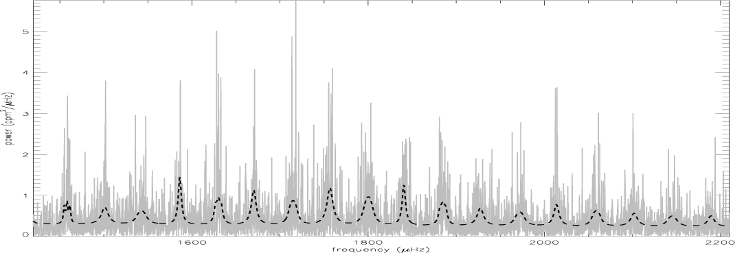 |
Figure 9:
HD 49933 power spectrum with
|
| Open with DEXTER | |
6 Conclusions and perspectives
We have presented a Bayesian analysis using an MCMC technique to infer mode parameters of solar-like oscillators, and applied it to the case of HD 49933. A global fitting strategy was adopted, taking into account the mode visibility dependence upon stellar inclination and the rotational mode splitting. The approach used here allows a global perspective of the fitted parameters thanks to the sampling of the probability density functions of these parameters and to the full implementation of our a priori physical knowledge of the object as a solar-type star.
The simulations show that this approach provides reliable parameter estimations
with a high robustness at low signal-to-noise ratio. Indeed, the systematic exploration of parameter space allows the method to avoid the local maxima encountered in MLE or MAP and permits us to obtain global information about the pdf of the parameters for the spectrum model tested.
One of the greatest difficulties encountered is the identification of the observed peaks in the Fourier spectrum with modes of given degree l.
The pdf sampling using parallel tempering gives the most probable model
thanks to the global likelihood calculation. As explained in Sect. 5, the estimated probability for each possible mode identification is more ambiguous than was shown by Appourchaux et al. (2008). In a statistical view, the best model is the mode identification A with only the l=0 and l=1 modes (
![]() ,
cf. Table 5). Gruberbauer et al. (2009)
also favor a model with these modes, but using a more heuristic approach, without taking into account the effects of rotation on the spectrum (and thus the effect of a star's inclination angle on the mode components relative heights).
However, the two models with modes of degree up to 2 (
,
cf. Table 5). Gruberbauer et al. (2009)
also favor a model with these modes, but using a more heuristic approach, without taking into account the effects of rotation on the spectrum (and thus the effect of a star's inclination angle on the mode components relative heights).
However, the two models with modes of degree up to 2 (
![]() and
and
![]() )
have comparable probabilities. The identification B, with only l=0 and l=1 modes (
)
have comparable probabilities. The identification B, with only l=0 and l=1 modes (
![]() ), is highly improbable. The low probability differences between the 3 most probable models prevents any definitive conclusion on the mode identification. The model
), is highly improbable. The low probability differences between the 3 most probable models prevents any definitive conclusion on the mode identification. The model
![]() is respectively only 2.7 and 4.5 times more probable than
is respectively only 2.7 and 4.5 times more probable than
![]() and
and
![]() .
We consider these factors not large enough to reject these models including l=2 modes. The model
.
We consider these factors not large enough to reject these models including l=2 modes. The model
![]() being 110 times less probable than
being 110 times less probable than
![]() ,
it can be definitely rejected. We have to emphasize that even if statistically speaking the most probable model does not include l=2 modes, it is unlikely in a physical view to not have l=2 modes excited (while l=1 are) for a solar like star in the main sequence. It would have been possible to take this hypothesis into account in the priors, but here, we have prefered to consider all the models as equally probable.
,
it can be definitely rejected. We have to emphasize that even if statistically speaking the most probable model does not include l=2 modes, it is unlikely in a physical view to not have l=2 modes excited (while l=1 are) for a solar like star in the main sequence. It would have been possible to take this hypothesis into account in the priors, but here, we have prefered to consider all the models as equally probable.
 |
Figure 10:
HD 49933 power spectrum and echelle diagram for
|
| Open with DEXTER | |
For example, these probabilities result from no informative a priori on the star inclination angle and on the relatives heights of the modes. However, one should note that identification B leads to a star inclination angle coherent with independent determinations of this angle (see Sect. 5) and also to relative heights more compatible with the expected values from solar observations. We have to stress that if we had applied an informative prior on the angle and/or on the relative heights, then it is possible that the model
![]() would have overruled the model
would have overruled the model
![]() .
Moreover we remind the reader that the estimated error on the determination of the probability is of
.
Moreover we remind the reader that the estimated error on the determination of the probability is of
![]() .
.
The present analysis could certainly be extended, for example by quantitatively evaluating the impact of the background model choice on the identification. The probabilistic Bayesian approach used here could be used to evaluate the relevance of the background description.
However, we think that, at the present stage, MCMC sampling is mainly useful in low signal-to-noise conditions to bring more information than classical approaches like MLE or MAP techniques do.
Acknowledgements
O.B. thanks Marie-Jo Goupil and Marc-Antoine Dupret for discussions about stellar theoretical modeling, and Reza Samadi for helpful discussions. Many thanks from all of us to John Leibacher for very instructive comments and Lucinda Croft for her help.
Appendix A: Technical aspects
A.1 Basic algorithm description
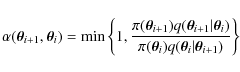
The Metropolis-Hasting (MH) algorithm (Hastings 1970; Metropolis et al. 1953) is the most commonly used MCMC algorithm because of its ease of implementation. We have already described the main advantages of the MCMC algorithm for the sampling of the space of the fitted parameters. Here we address its inherent difficulties and the solutions to manage these difficulties.
Considering
![]() ,
the distribution we want to sample (also called ``distribution of interest''), we define a probability transition function
,
the distribution we want to sample (also called ``distribution of interest''), we define a probability transition function
![]() from an initial parameter set
from an initial parameter set
![]() to a new proposed set
to a new proposed set
![]() ,
in order to sample the space of parameters
,
in order to sample the space of parameters
 |
(A.1) |
where
A.2 Gaussian proposal covariance matrix adjustment
In the present analysis, we used a Gaussian proposal distribution
![]() :
the trial set of parameter
:
the trial set of parameter ![]() is created by the scheme
is created by the scheme
![]() .
Then, an important task for a correct sampling consists of adjusting the covariance matrix
.
Then, an important task for a correct sampling consists of adjusting the covariance matrix
![]() of this multidimensional Gaussian function (if all parameters were independent, only the diagonal terms would be non-zero). Indeed, the acceptance rate depends directly on
of this multidimensional Gaussian function (if all parameters were independent, only the diagonal terms would be non-zero). Indeed, the acceptance rate depends directly on
![]() .
If
.
If
![]() is too low then few samples are accepted and the typical computing time to sample the distribution of interest will be large. Conversely, a high
is too low then few samples are accepted and the typical computing time to sample the distribution of interest will be large. Conversely, a high
![]() introduces a high correlation between two successive samples and the sampling process can be easily trapped in local maxima of the distribution of interest. Roberts et al. (1997) empirically show for high dimensional models that the best sampling is obtained for an acceptance rate of around 25%. Many authors recommend a rate between 20% and 50%.
introduces a high correlation between two successive samples and the sampling process can be easily trapped in local maxima of the distribution of interest. Roberts et al. (1997) empirically show for high dimensional models that the best sampling is obtained for an acceptance rate of around 25%. Many authors recommend a rate between 20% and 50%.
The manual adjustment of such a matrix is easy if we deal with a few parameters but becomes difficult to manage in high dimensional cases. A way to automate the matrix determination process is to use Adaptive MCMC. Adaptive MCMC runs a second process, in parallel to the sampling process, that adapts the covariance matrix continuously. Many Adaptive MCMCs have been proposed. The one used in this paper was inspired by the work of Atchadé (2006). It uses a Robbins-Monro type algorithm, widely used to calculate numerical solutions of differential equations (Robbins & Monro 1951).
Initially,
![]() is defined as diagonal with coefficient
is defined as diagonal with coefficient
![]() where
where
![]() the Kronecker symbol and
the Kronecker symbol and
![]() the initial variance for the ith element of the parameter vector.
The initial parameter values are set at the center of the prior range and
the initial variance for the ith element of the parameter vector.
The initial parameter values are set at the center of the prior range and ![]() at 10% of their values. During the acceptance-rate adapting phase (or learning phase), even the non-diagonal terms are adjusted, taking into account a hypothetical correlation between parameters to enhance the sampling.
Despite its name, an Adaptive MCMC is not a Markovian process as the i+1 state depends not only on the previous one i, but also on all previous states
i-1,i-2,.... There is no guarantee that the sampling will be done according to the distribution of interest. To avoid this problem, we simply stop the learning process when the acceptance rate is reasonable, i.e. is within 20% of the optimal acceptance rate.
at 10% of their values. During the acceptance-rate adapting phase (or learning phase), even the non-diagonal terms are adjusted, taking into account a hypothetical correlation between parameters to enhance the sampling.
Despite its name, an Adaptive MCMC is not a Markovian process as the i+1 state depends not only on the previous one i, but also on all previous states
i-1,i-2,.... There is no guarantee that the sampling will be done according to the distribution of interest. To avoid this problem, we simply stop the learning process when the acceptance rate is reasonable, i.e. is within 20% of the optimal acceptance rate.
A.3 Parallel tempering
The MH algorithm can encounter difficulties for multimodal distributions, in particular if the maxima are far from one other. In order to efficiently sample the entire parameter space, a solution was proposed by Jennison (1993). It consists of the launching of multiple parallel MCMC processes. Each process has a different distribution according to a power law
![]() where Tk is called the temperature of the chain k.
The higher the temperature, the flatter is the distribution. In a flat distribution, the potential barrier between distant maxima is lowered and the transitions in the parameter space are easier.
where Tk is called the temperature of the chain k.
The higher the temperature, the flatter is the distribution. In a flat distribution, the potential barrier between distant maxima is lowered and the transitions in the parameter space are easier.
At each iteration i, a random mix is made among neighboring chains: two chains k and k+1 are mixed with the probability
 |
(A.2) |
The temperatures follow a geometric law:
Thanks to this numerical method, MCMC simulations can be used to evaluate the odds ratio (Eq. (9)) through the calculation of Eq. (11). As shown by Gregory (2005b),
![\begin{displaymath}\ln[P(y\vert M_j,I)]=\int_0^1 \langle \ln[\pi(y\vert M_j,\vec{\theta},I)]\rangle_{\beta}{\rm d}\beta
\end{displaymath}](/articles/aa/full_html/2009/40/aa11657-09/img202.png) |
(A.3) |
where
When
![]() ,
the likelihood distribution is flat and the target distribution
,
the likelihood distribution is flat and the target distribution
![]() is dominated by the priors. Conversely, Tk=1 corresponds to the distribution of interest.
is dominated by the priors. Conversely, Tk=1 corresponds to the distribution of interest.
To summarize, we proceed as follows: for each chain at temperature
![]() ,
we calculate the mean value of the conditional likelihood and then we evaluate the log probability
,
we calculate the mean value of the conditional likelihood and then we evaluate the log probability
![]() by generating and integrating an interpolated function of
by generating and integrating an interpolated function of
![]() .
.
A.4 Possible improvements
From a technical point of view, improvements can be made. The probability calculation is a crucial aspect which has only been sketched. Indeed we use a random walk algorithm and the probability is subject to fluctuations as a function of the number of samples, the number of parallel chains and of their distribution (depending on the chosen temperature set). It is necessary to investigate these three points to make sure of the robustness of the probability calculation.
Concerning the execution speed, the Bayesian analysis coupled with a MCMC sampling for large data sets and a large number of parameters is costly in terms of computation time. In the present analysis of HD 49933, the computation time is of the order of a week per model (on a personal computer). This heavy computation limits the degree of complexity possible of the models investigated to describe the observed spectrum.
References
- Aigrain, S., Favata, F., & Gilmore, G. 2004, A&A, 414, 1139 [NASA ADS] [CrossRef] [EDP Sciences] (In the text)
- Anderson, E. R., Duvall, T. L., & Jefferies, S. M. 1990, ApJ, 364, 699 [NASA ADS] [CrossRef]
- Appourchaux, T., Gizon, L., & Rabello-Soares, M.-C. 1998, A&AS, 132, 107 [NASA ADS] [CrossRef] [EDP Sciences]
- Appourchaux, T., Michel, E., Auvergne, M., et al. 2008, A&A, 488, 705 [NASA ADS] [CrossRef] [EDP Sciences] (In the text)
- Atchadé, Y. F. 2006, Meth. Comp. In Applied Probab., 8, 235 [CrossRef] (In the text)
- Benomar, O. 2008, CoAst, 157 (In the text)
- Brewer, B. J., Bedding, T. R., Kjeldsen, H., & Stello, D. 2007, ApJ, 654, 551 [NASA ADS] [CrossRef] (In the text)
- Carrier, F., Kjeldsen, H., Bedding, T. R., et al. 2007, A&A, 470, 1059 [NASA ADS] [CrossRef] [EDP Sciences] (In the text)
- Duvall, T., & Harvey, J. 1986, NATO ASI Series C: Math. Phys. Sci., 169, 105 (In the text)
- Gizon, L., & Solanki, S. K. 2003, ApJ, 589, 1009 [NASA ADS] [CrossRef] (In the text)
- Gregory, P. C. 2005a, ApJ, 631, 1198 [NASA ADS] [CrossRef] (In the text)
- Gregory, P. C. 2005b, Bayesian Logical Data Analysis for the Physical Sciences: A Comparative Approach with Mathematica Support (Cambridge University Press) (In the text)
- Gruberbauer, M., Kallinger, T., & Weiss, W. W., et al. 2009, A&A, accepted (In the text)
- Harvey, J. 1985, ESA SP, 235, 199 [NASA ADS] (In the text)
- Hastings, W. 1970, Biometrika, 57, 97 [CrossRef]
- Jeffrey, A. 1961, (Cambridge University Press) (In the text)
- Jennison, C. 1993, J. Roy. Statist. Soc. Series B, 55, 54 (In the text)
- Metropolis, N., Rosenbluth, A., & Rosenbluth, M. 1953, J. Chem. Phys., 21, 188 [CrossRef]
- Mosser, B., Bouchy, F., Catala, C., et al. 2005, A&A, 431, L13 [NASA ADS] [CrossRef] [EDP Sciences] (In the text)
- Parkinson, D., Mukherjee, P., & Liddle, A. R. 2006, Phys. Rev. D, 73, 123523 [NASA ADS] [CrossRef] (In the text)
- Robbins, H., & Monro, S. 1951, Ann. Math. Stat., 22, 400 [CrossRef] (In the text)
- Roberts, G. O., Gelman, A., & Gilks, W. R. 1997, Ann. Appl. Prob., 7, 110 [CrossRef] (In the text)
- Solano, E., Catala, C., Garrido, R., et al. 2005, AJ, 129, 547 [NASA ADS] [CrossRef] (In the text)
- Thévenin, F., Bigot, L., Kervella, P., et al. 2006, Mem. Soc. Astron. Ital., 77, 411 [NASA ADS] (In the text)
- Toutain, T., & Fröhlich, C. 1992, A&A, 257, 287 [NASA ADS]
- Toutain, T., & Gouttebroze, P. 1993, A&A, 268, 309 [NASA ADS] (In the text)
Online Material
Table 10:
HD 49933 frequencies and height-to-noise posterior estimates for l=0 and l=1 modes for the
![]() model. n is given supposing
model. n is given supposing
![]() .
H/N represents the height-to-noise ratio in the power spectrum.
.
H/N represents the height-to-noise ratio in the power spectrum.
Table 11:
Height and width posterior estimates for HD 49933 for the model
![]() .
n is given for the l=0 modes.
.
n is given for the l=0 modes.
Table 12:
Energy posterior estimates for HD 49933, model
![]() .
n is given for the l=0 modes.
.
n is given for the l=0 modes.
Table 13:
HD 49933 frequencies and height-to-noise posterior estimates for the l=0 and l=1 modes for the
![]() model. n is given supposing
model. n is given supposing
![]() .
H/N represents the height-to-noise ratio in the power spectrum.
.
H/N represents the height-to-noise ratio in the power spectrum.
Table 14:
Height and width posterior estimates for HD 49933 for the model
![]() .
n is given for the l=0 modes.
.
n is given for the l=0 modes.
Table 15:
Energy posterior estimates for HD 49933, model
![]() .
n is given for the l=0 modes.
.
n is given for the l=0 modes.
 |
Figure 11:
HD 49933 power spectrum and echelle diagram for
|
| Open with DEXTER | |
 |
Figure 12:
HD 49933 power spectrum and echelle diagram for
|
| Open with DEXTER | |
Footnotes
- ... approach
- The CoRoT space mission, launched on 2006 December 27, was developed and is operated by the CNES, with participation of the Science Programs of ESA, ESA's RSSD, Austria, Belgium, Brazil, Germany and Spain.
- ...
- Tables 10 to 15 and Figs. 11, 12 are only available in electronic form at http://www.aanda.org
All Tables
Table 1: Input parameters used for the simulated spectra.
Table 2:
Priors used for the analysis of the simulated spectra for the inclination angle i, the rotational splitting
![]() ,
the large separation
,
the large separation ![]() (Eq. (2)) and the small separation
(Eq. (2)) and the small separation
![]() (Eq. (15)).
(Eq. (15)).
Table 3:
Top: model odds ratio
![]() for scenario 1 to 5 (which include l=2 modes). Bottom: odds ratio for scenario 6, comparing 4 models (identifications A and B, with or without l=2).
for scenario 1 to 5 (which include l=2 modes). Bottom: odds ratio for scenario 6, comparing 4 models (identifications A and B, with or without l=2).
Table 4:
Priors used for HD 49933 data analysis.
![]() is the rotational splitting, i the star inclination angle,
is the rotational splitting, i the star inclination angle,
![]() the small frequency separation,
the small frequency separation, ![]() the large separation. The value of
the large separation. The value of ![]() and D0 depend on the model and set the position of the first prior frequency (see Eq. (2)).
and D0 depend on the model and set the position of the first prior frequency (see Eq. (2)).
Table 5: Model odds ratio and estimated probability for HD 49933 spectrum analysis. The value of the matrix represents the odds ratio.
Table 6:
HD 49933 frequencies and height-to-noise posterior estimates for l=0 and l=1 modes for the
![]() model.
model.
Table 7: Height and width posterior estimates for HD 49933 for the most probable model. n is given for the l=0 modes.
Table 8: Energy posterior estimates for HD 49933. n is given for the l=0 modes.
Table 9:
Global parameter posterior estimates for HD 49933. i represents the inclination angle of the star.
![]() is the rotational splitting, Vl=1 and Vl=2 the relative height of l=1 and l=2 modes, respectively.
is the rotational splitting, Vl=1 and Vl=2 the relative height of l=1 and l=2 modes, respectively. ![]() represent the large separation.
represent the large separation.
Table 10:
HD 49933 frequencies and height-to-noise posterior estimates for l=0 and l=1 modes for the
![]() model. n is given supposing
model. n is given supposing
![]() .
H/N represents the height-to-noise ratio in the power spectrum.
.
H/N represents the height-to-noise ratio in the power spectrum.
Table 11:
Height and width posterior estimates for HD 49933 for the model
![]() .
n is given for the l=0 modes.
.
n is given for the l=0 modes.
Table 12:
Energy posterior estimates for HD 49933, model
![]() .
n is given for the l=0 modes.
.
n is given for the l=0 modes.
Table 13:
HD 49933 frequencies and height-to-noise posterior estimates for the l=0 and l=1 modes for the
![]() model. n is given supposing
model. n is given supposing
![]() .
H/N represents the height-to-noise ratio in the power spectrum.
.
H/N represents the height-to-noise ratio in the power spectrum.
Table 14:
Height and width posterior estimates for HD 49933 for the model
![]() .
n is given for the l=0 modes.
.
n is given for the l=0 modes.
Table 15:
Energy posterior estimates for HD 49933, model
![]() .
n is given for the l=0 modes.
.
n is given for the l=0 modes.
All Figures
| |
Figure 1: a) Smoothed power spectrum of HD 49933, showing activity (dot-dashed line) and granulation (solid line) backgrounds and stellar modes.The modes are first modeled by a Gaussian (solid blue curve). b) Mode frequency range with frequency priors (l=0: red dash line; l=1: green dot line) for the mode identification A. |
| Open with DEXTER | |
| In the text | |
| |
Figure 2:
l=2 mode relative height from simulation (scenario 3) for the correct identification a) and for the wrong identification b). In the correct identification, due to the l=0 and l=2 mode superposition, the relative height H2/H0 is underestimated by 30%. In the wrong identification, the distribution of the height follows the |
| Open with DEXTER | |
| In the text | |
| |
Figure 3:
HD 49933 typical frequency, height, width and amplitude pdf (here for model
|
| Open with DEXTER | |
| In the text | |
| |
Figure 4:
Comparison of the output and input values for simulated spectra, for scenario 3 ( a), b), c)) and for scenario 4 ( d), e), f)). The box represent the 68.3% confidence interval (1 |
| Open with DEXTER | |
| In the text | |
| |
Figure 5:
HD 49933 echelle diagram for the model
|
| Open with DEXTER | |
| In the text | |
| |
Figure 6:
Estimated heights, width and amplitude for model
|
| Open with DEXTER | |
| In the text | |
| |
Figure 7:
Estimated heights, width and amplitude for model
|
| Open with DEXTER | |
| In the text | |
| |
Figure 8:
Posterior probability density function for the rotational splitting and the inclination angle of HD 49933 for each possible mode identification including l=2 for model
|
| Open with DEXTER | |
| In the text | |
| |
Figure 9:
HD 49933 power spectrum with
|
| Open with DEXTER | |
| In the text | |
| |
Figure 10:
HD 49933 power spectrum and echelle diagram for
|
| Open with DEXTER | |
| In the text | |
| |
Figure 11:
HD 49933 power spectrum and echelle diagram for
|
| Open with DEXTER | |
| In the text | |
| |
Figure 12:
HD 49933 power spectrum and echelle diagram for
|
| Open with DEXTER | |
| In the text | |
Copyright ESO 2009
Current usage metrics show cumulative count of Article Views (full-text article views including HTML views, PDF and ePub downloads, according to the available data) and Abstracts Views on Vision4Press platform.
Data correspond to usage on the plateform after 2015. The current usage metrics is available 48-96 hours after online publication and is updated daily on week days.
Initial download of the metrics may take a while.