| Issue |
A&A
Volume 506, Number 1, October IV 2009
The CoRoT space mission: early results
|
|
|---|---|---|
| Page(s) | 519 - 534 | |
| Section | Catalogs and data | |
| DOI | https://doi.org/10.1051/0004-6361/200911618 | |
| Published online | 29 April 2009 | |
The CoRoT space mission: early results
Automated supervised classification of variable stars in the CoRoT programme
Method and application to the first four exoplanet fields![[*]](/icons/foot_motif.png) ,
,
J. Debosscher1 - L. M. Sarro2 - M. López3 - M. Deleuil4 - C. Aerts1,5 - M. Auvergne6 - A. Baglin6 - F. Baudin18 - M. Chadid8 - S. Charpinet9 - J. Cuypers7 - J. De Ridder1 - R. Garrido10 - A. M. Hubert11 - E. Janot-Pacheco12 - L. Jorda4 - A. Kaiser13 - T. Kallinger13 - Z. Kollath14 - C. Maceroni15 - P. Mathias8 - E. Michel6 - C. Moutou4 - C. Neiner11 - M. Ollivier18 - R. Samadi6 - E. Solano3 - C. Surace4 - B. Vandenbussche1 - W. W. Weiss13
1 -
Instituut voor Sterrenkunde, Catholic University of Leuven, Celestijnenlaan 200D, 3001 Leuven, Belgium
2 - Dpt. de Inteligencia Artificial , UNED, Juan del Rosal, 16, 28040 Madrid, Spain
3 - LAEX-CAB (INTA-CSIC), Postal address.- LAEFF, European Space Astronomy Center (ESAC), PO Box 78, 28691 Villanueva de la Cañada, Madrid, Spain
4 - LAM, UMR 6110, CNRS/Univ. de Provence, 38 rue F. Joliot-Curie, 13388 Marseille, France
5 - Department of Astrophysics, Radboud University Nijmegen, PO Box 9010, 6500 GL Nijmegen, The Netherlands
6 - LESIA, UMR8109, Université Pierre et Marie Curie, Université Denis Diderot, Observatoire de Paris, 92195 Meudon Cedex, France
7 - Royal Observatory of Belgium, Ringlaan 3, 1180 Brussel, Belgium
8 - Observatoire de la Côte d'Azur, Université Nice Sophia-Antipolis, UMR 6525. Parc Valrose, 06108 Nice, France
9 - Laboratoire d'Astrophysique de Toulouse-Tarbes, Université de Toulouse, CNRS, 14 Av. E. Belin, 31400 Toulouse, France
10 - Instituto de Astrofísica de Andalucía-CSIC, Apdo 3004, 18080 Granada, Spain
11 - GEPI, Observatoire de Paris, CNRS, Université Paris Diderot, 5 place Jules Janssen, 92195 Meudon Cedex, France
12 - Universidade de São Paulo, Instituto de Astronomia, Geofísica e Ciências Atmosféricas - IAG, Departamento de Astronomia, Rua do Matão 1226, 05508-900 São Paulo, Brazil
13 - Department of Astronomy, University of Vienna, Türkenschanzstrasse 17, 1180 Wien, Austria
14 - Konkoly Observatory, 1525 Budapest, PO Box 67., Hungary
15 - INAF - Osservatorio Astronomico di Roma via Frascati 33, 00040 Monteporzio C. (RM), Italy
16 - Laboratorio de Astrofísica Espacial y Física Fundamental, INSA, Apartado de Correos 50727, 28080 Madrid, Spain
17 - Spanish Virtual Observatory, INTA, Apartado de Correos 50727, 28080 Madrid, Spain
18 - IAS, Université Paris XI, 91405 Orsay, France
Received 2 January 2009 / Accepted 12 March 2009
Abstract
Aims. In this work, we describe the pipeline for the fast supervised classification of light curves observed by the CoRoT exoplanet CCDs. We present the classification results obtained for the first four measured fields, which represent a one-year in-orbit operation.
Methods. The basis of the adopted supervised classification methodology has been described in detail in a previous paper, as is its application to the OGLE database. Here, we present the modifications of the algorithms and of the training set to optimize the performance when applied to the CoRoT data.
Results. Classification results are presented for the observed fields IRa01, SRc01, LRc01, and LRa01 of the CoRoT mission. Statistics on the number of variables and the number of objects per class are given and typical light curves of high-probability candidates are shown. We also report on new stellar variability types discovered in the CoRoT data. The full classification results are publicly available.
Key words: stars: variables: general - stars: binaries: general - techniques: photometric - methods: statistical - methods: data analysis
1 Introduction
As an important by-product of the CoRoT mission, a database of light curves with excellent time-sampling and unprecedented photometric precision is produced. Hidden in this database are many light curves of variable stars, of both known and still unknown nature.
Before any science can be done with the data, scientists need to identify their objects of study. Since the database is large (![]() 40 000 light curves), having to extract these targets in a manual way would be very time-consuming. Moreover, scientists interested in different objects would each have to screen the whole database again. Automated classification methods can save us lots of time, they are repeatable, and they are not subject to the human subjectivity inherent in manual methods.
40 000 light curves), having to extract these targets in a manual way would be very time-consuming. Moreover, scientists interested in different objects would each have to screen the whole database again. Automated classification methods can save us lots of time, they are repeatable, and they are not subject to the human subjectivity inherent in manual methods.
Table 1: Basic properties of the data, coming from the first 4 exoplanet fields, having a 512 s nominal sampling time.
In this work, we describe an automated supervised classification method, developed in the framework of the CoRoT mission. The basis of the method has been described in detail in Debosscher et al. (2007), hereafter denoted as Paper I, and its application to the OGLE database is described in Sarro et al. (2009a), hereafter denoted as Paper II. In the latter, we have shown that the classifiers are capable of assigning probabilistic class labels, which are highly reliable for the classical variables studied most in the literature and for eclipsing binaries. We also pointed out how we plan to improve the classifiers and the training set containing the necessary class definitions for a supervised classifier. The classifiers presented here are an adaptation of the classifiers presented in Paper I, with the goal of optimizing their performance when applied to CoRoT data. Hereafter, we refer to this adapted version as the ``CoRoT Variability Classifier'' (CVC).We present the results obtained with the CVC for the first four exoplanet fields measured by CoRoT (IRa01, LRc01, SRc01, and LRa01, see below for an explanation of the field designations). Estimates of the number of variables for every field are given, as well as statistics on the population of the different classes considered by the CVC. Light curves of the best candidates are shown, together with phase plots made with the detected dominant frequency. We also report on the presence of new variability types or border cases of already known variability types. A description is given of the classification output, as will be made available in the so-called N3 product delivery in the public database of the mission. This should allow users of the catalogue to interpret the classification results in such a way, that they can create candidate lists of their science objects according to some pre-defined criteria, without having to know all details of the classification process.
2 Data description
The data treated here include all the calibrated (i.e. N2-level) light curves that have been measured by the CoRoT exoplanet CCDs during the IRa01, LRc01, SRc01, and LRa01 observing runs (visual magnitudes of the stars roughly between 12 and 15.5). Some basic properties of the datasets are listed in Table 1. The time sampling of the light curves is 32 s, but for the majority of the light curves, an average is taken over 16 such measurements, resulting in an effective time resolution of 512 s. For a fraction of the light curves (or parts of some light curves), the original 32 s sampling is retained. These are high priority targets that have been measured in oversampling mode.
Prior to the data analysis, we removed all measurements having non-zero quality flags in the N2 product delivery, retaining only valid flux measurements. These flagged measurements include, e.g., measurements taken during SAA (South-Atlantic Anomaly) passages. It concerns roughly 1.8% of the data for the worst cases. The removal of these bad datapoints causes the equidistance of the time series to be lost and changes the window function. This has to be taken into account in the analysis (e.g. FFT can no longer trivially be used, as equidistancy is needed here). The brighter stars in the exoplanet fields are measured in three colours (RGB), obtained using a dispersion device. The goal is to distinguish between planetary transits and stellar activity, the latter being highly chromatic. The dispersed light is integrated in these RGB bands onboard, according to a mask selected from a set of 256 predefined ones, depending on target characteristics, such that approximately 40% of the light falls in the R band, 30% in the G band, and 30% in the B band. Thus, the definition of the bands (their limits in wavelengths) are target dependent. Since the fraction of the total stellar flux in every colour channel is held constant, we cannot use the fluxes in the three channels to obtain calibrated colour information on the stars. When dealing with chromatic light curves, we thus sum up the fluxes in the three channels and use the resulting ``white'' flux for our purposes.
3 Computation of the classification parameters from the light curves
The light curve analysis method is basically the same as described in Paper I. However, some adaptations had to be made to account for some unavoidable systematics encountered in the CoRoT N2 data: trends in the light curves due to changes in the amount of incident stray light during the run, periodic changes in flux caused by the satellite orbit, and discontinuities in the light curves due to cosmic ray hits on the CCDs. To remove the systematic trends, we subtracted a second-order polynomial from the light curves, where the coefficients are computed for every light curve separately. We note that some objects such as Be-stars or long-period variables can show intrinsic trends in their light curves. It is clear that, in some cases, we remove part of these real trends as well. This is undesirable, since the presence of such an intrinsic trend can contain important astrophysical information on the type of object. However, we cannot avoid this for the moment, because of the presence of the instrumental trends. Since it is essential that pulsation frequencies are recovered as much as possible, we preferred to subtract the trends for each object, prior to frequency analysis.
Frequency analysis was then performed, using a Lomb-Scargle periodogram (Scargle 1982; Lomb 1976). The frequency range and resolution of the periodogram was determined for each light curve individually, because the time sampling is not the same for all the light curves. As a lower frequency limit, we originally used
![]() ,
with
,
with
![]() the total time span of the observations. The upper limit fN varies from light curve to light curve, with
the total time span of the observations. The upper limit fN varies from light curve to light curve, with
![]() for a 512 s sampled light curve, and
for a 512 s sampled light curve, and
![]() for the 32 s sampled light curves. For the frequency resolution, we took
for the 32 s sampled light curves. For the frequency resolution, we took
![]() (for IRa01 and SRc01) or
(for IRa01 and SRc01) or
![]() (LRc01 and LRa01, for CPU reasons). As can be seen from these expressions, the frequency resolution depends on the total time span of the observations. This is necessary, since the width of the spectral peaks can be shown to be equal to
(LRc01 and LRa01, for CPU reasons). As can be seen from these expressions, the frequency resolution depends on the total time span of the observations. This is necessary, since the width of the spectral peaks can be shown to be equal to
![]() (strictly speaking this is only valid for equidistant time-series). In total, we determined three different frequencies per object, in an iterative scheme of spectral peak selection and prewhitening. Every prewhitening step consists in subtracting a harmonic least squares fit of the form
(strictly speaking this is only valid for equidistant time-series). In total, we determined three different frequencies per object, in an iterative scheme of spectral peak selection and prewhitening. Every prewhitening step consists in subtracting a harmonic least squares fit of the form
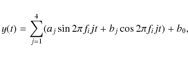 |
(1) |
with i=1,2,3. The fitting coefficients obtained in each step provide us with an overall good description of the variability present in the light curves. The detected frequencies and fitting coefficients are then transformed into suitable classification parameters (depending on the classifier used). It is crucial that these parameters describe the intrinsic variability of the measured object as precisely as possible and are not contaminated by instrumental effects (any signature in the light curve not caused by the object's real variability).
All classification results presented in this work are obtained using attributes, derived from the abovementioned light curve parameters. An extended version of our classifiers can handle colour attributes such as B-V magnitudes if they are available. At this stage, however, we preferred not to include any spectral attributes in the classifiers for the CoRoT data, because no reliable colours (such as Johnson B-V or Strömgren b-y) are available yet for the majority of the stars described here. The use of an unreliable colour index can have a very bad influence on the classification results so should be avoided. Finally, the unprecedented photometric precision and continuous time coverage of the CoRoT data make it worthwhile to investigate how well the classes can be separated on the basis of the light curve information alone.
4 Avoiding instrumental effects
Every photometric database unavoidably has its own instrumental systematics, causing a blind application of the classification codes to produce suboptimal results. Fortunately, the large number of light curves in the CoRoT database allows us to identify the most obvious systematics.
After a first exploratory analysis, we found that the major contamination of the light curve parameters was caused by the orbital frequency (around 13.97 d-1) and its higher harmonics. Even though the amplitudes of these peaks are low (typically below 900 parts per million, ppm hereafter), they clearly stand far above the low CoRoT noise level. Spectral peaks related to the orbital frequency were therefore ignored in the frequency analysis procedure.
Other clear systematics in the light curves are the long-term trends. Even though we first subtracted a second order polynomial prior to frequency analysis, a lot of significant peaks remained in the low frequency part of the amplitude spectrum. For a large number of light curves, the highest peak in the entire amplitude spectrum stem from these trends, especially for the long run data. To avoid these being selected as frequencies, hence as classification attributes, we ignored the lowest frequency part in the spectrum. The lower limit was adjusted, depending on the observing run. As a drawback, we were not able to correctly detect pulsators with periods longer than typically those of classical Cepheids. This is fine, given that the CoRoT target selection avoided supergiant variables anyhow.
Additional systematics were identified in some of the light curves. Depending on the run, spurious frequencies around 1 d-1 were detected. They are related to variations in the amount of received stray light due to the Earth's day/night cycle. These can cause sidelobes to appear around the orbital peaks as well (at 13.97-1 d-1 and 13.97+1 d-1, the same occurs for the higher harmonics). The amplitudes of those peaks are usually much less than the amplitudes of the orbital harmonic frequencies. We chose not to exclude those as well, since this would increase the risk of missing real frequencies. Rejecting frequencies close to 1 d-1 risks missing real pulsation frequencies of B or F-type pulsators such as slowly pulsating B (SPB) or ![]() -Doradus stars, which are among the most interesting targets for asteroseismology.
-Doradus stars, which are among the most interesting targets for asteroseismology.
5 The CoRoT variability classifier
After the light curve analysis process, the parameters are transformed into suitable classification attributes and are used as input for two different supervised classification methods: multistage Bayesian networks (MSBN) and Gaussian mixtures (GM). Both methods, as well as the construction of the original common training set, have been described in detail in Paper I, to which we refer for details. The same methodology was used as a starting point for classifying the CoRoT exoplanet data. After a first evaluation of the results, adaptations were made in order to optimize the performance when applied to CoRoT data. These include improving the training set, investigating new attributes, better separating the multiperiodic variables, and including new classes.
Table 2: Variability classes whose definition stars have been extended/replaced with CoRoT data, and the number of definition CoRoT light curves used.
![\begin{figure}
\par\includegraphics[width=16cm,clip]{1618f1.ps}
\end{figure}](/articles/aa/full_html/2009/40/aa11618-09/img20.png) |
Figure 1: Some CoRoT light curves of low-amplitude periodic variables, measured in the IRa01. The original N2 level light curve is shown with a phase plot after detrending, made with the dominant detected frequency (given below the plot). |
| Open with DEXTER | |
5.1 Adapting the training set
Ideally, a training set should be constructed from data measured with the same instrument as the data to be classified. This is usually not feasible because constructing a completely new training set for every new database would be very time-consuming. Moreover, the database will most often not contain enough good candidate class members, to be used for training. Luckily, as shown in Paper II, there is no need to construct a completely new training set every time a new database is classified, provided that the kind and quality of the data are not too different.
In a first application of our codes to the CoRoT data, we used the original training set as defined in Paper I. This already gave satisfactory results for the recognised classes such as eclipsing binaries, classical pulsators, and non-radial pulsators, such as SPB and ![]() -Scuti stars. It was clear, however, that misclassifications occurred because of the difference in quality and systematics of the data present in the training set and the much higher quality CoRoT data.
-Scuti stars. It was clear, however, that misclassifications occurred because of the difference in quality and systematics of the data present in the training set and the much higher quality CoRoT data.
We improved the training set in an iterative way. Candidate lists obtained with the first version of the classifiers and the old training set were used to select bona-fide (or at least very probable) class members among the CoRoT targets, suitable for inclusions in the training set. Unfortunately, this was only possible for some classes (listed in Table 2). We hope to include CoRoT members for other classes in the future, when more data is available.
Apart from improving the already existing class definitions, we also included a new class in the training set: low-amplitude periodic variables (LAPV). The definition objects for this class include candidate low-amplitude Cepheids, but also stars showing very regular periodic light variations due to rotation (e.g. stellar spots). The latter can be difficult to distinguish from a Cepheid light curve, without additional colour information. The low-amplitude Cepheids were already known as a class of stars (see Buchler et al. 2005), but it is only now with CoRoT that good quality light curves of low-amplitude variables have become available. The light curve shapes are very similar to those of Classical Cepheids, but the main pulsation amplitude is significantly lower. These pulsations are predicted by theory at the borders of the Cepheid instability strip. Figure 1 shows four light curves of low-amplitude periodic variables, measured in the IRa01 observing run. We also show a phase plot made with the dominant, detected frequency, after subtraction of a trend, if any. These light curves have been included in the LAPV class definition.
5.2 Adaptations of the classifiers
Apart from the necessary re-training of the classifiers after the extension of the training set with CoRoT data, the design of the classifiers was also adapted. The multi-stage design of the MSBN classifier was altered to include a new stage for a better separation of the multiperiodic variables (GDOR, DSCUT, SPB, BCEP, and PVSG). These changes, in combination with the new training set also largely solved the problem of some good SPB candidates being misclassified as ellipsoidal variables in the first version of the classifier.
We implemented a multistage approach for the GM classifier as well. It is just a simple two-stage design: the first stage attempts to separate the binaries from other variability types, using only a small set of attributes (frequency ratios and phase differences). The second stage attempts to separate all the other classes, using a different and larger set of attributes. This approach effectively increased the number of correct classifications for binaries.
6 The CoRoT N3 product description
In this section, we describe the CVC N3 product, to be made available to the scientific community along with the full CoRoT data release. The information present in the N3 product should allow scientists to make candidate lists of their objects of study and to obtain some basic light curve information. We recall that we did not perform detailed light curve modelling, only a basic one, sufficient for producing class memberships for each target. For every measured field, an ASCII file with CVC results will be delivered. The files contain one line per light curve, listing the following information in the columns:
- 1)
- objectname = CoRoT ID;
- 2-4)
- classprob1-3 = relative probabilities for three most likely class memberships, obtained with the MSBN classifier;
- 5-7)
- classcode1-3 = corresponding to the three most likely variability class memberships, in decreasing order of probability;
- 8-10)
- Pf1-3 = significance parameters for the three dominant frequencies f1, f2, f3 (probability);
- 11-13)
- f1-3 = three dominant independent frequencies f1, f2, f3 (units:
 );
);
- 14-17)
- amp11-14 = amplitude of f1, 2f1, 3f1, 4f1 (units: mag);
- 18-21)
- amp21-24 = amplitude of f2, 2f2, 3f2, 4f2 (units: mag);
- 22-25)
- amp31-34 = amplitude of f3, 2f3, 3f3, 4f3 (units: mag);
- 26-28)
- phdiff12-14 = phase of 2f1, 3f1, 4f1, if phase of f1=0 (units: rad);
- 29-32)
- phdiff21-24 = phase of f2, 2f2, 3f2, 4f2, if phase of f1=0 (units: rad);
- 33-36)
- phdiff31-34 = phase of f3, 2f3, 3f3, 4f3, if phase of f1=0 (units: rad);
- 37)
- varred = total variance reduction of the trend-subtracted light curve, after subtraction of the least-squares fits with the 3 frequencies and their harmonics (values between 0 and 1).
Table 3: The different variability classes considered by the CVC and our abbreviations.
6.1 Variability indicators and significance testing
The CVC N3 output includes significance parameters that allow users to select the clear variables, but also to have an idea of the significance of the 3 frequencies separately. These are the probability parameters Pf1, Pf2, and Pf3, one for every detected frequency. The derivation and interpretation of those parameters deserves some explanation. First of all, they are not to be interpreted as the probability that the found frequency is significant. These are P-values resulting from a statistical Fisher-test (F-test) on the ratio of the variance before and after subtracting a harmonic least-squares fit (for each of the frequencies f1, f2, and f3 separately). We use a single-tailed version of the test, since subtracting a least-squares fit always causes a reduction in variance.
The motivation to use an F-test is as follows.
Assume that a ``constant'' CoRoT light curve is generated by a Gaussian random process: each measurement is independently ``drawn'' from a Gaussian distribution N(![]() ,
,![]() ), where
), where ![]() and
and ![]() are identical for every measurement in the light curve (but are allowed to be different for other light curves). As it turns out, the assumption of Gaussian noise is a very reasonable one for the CoRoT light curves. Imagine we perform frequency analysis on such a constant light curve. We will always find a highest peak in the power spectrum, and we use the corresponding frequency to make a harmonic least-squares fit to the light curve. After subtracting the fit from the original data, we compare the variance of the data before and after subtracting the fit. We expect that the variance will not be significantly reduced in this case, because no periodicity is present in the data, and we just picked a frequency corresponding to the highest noise peak in the spectrum. On the other hand, imagine that a clear periodic signal is present in the light curve, on top of the Gaussian noise. In this case, we will see a clear peak in the power spectrum, and subtracting a harmonic fit with the corresponding frequency will significantly reduce the variance of the data.
We test the null-hypothesis (H0) of equal variances in the data before and after subtraction of a periodic signal. The resulting P-values can now be used to have an idea of the significance of the subtracted signal. P-values close to 1 indicate that we should not reject the null-hypothesis, meaning that we are dealing with an insignificant reduction in variance, hence an insignificant signal. P-values close to zero indicate that we should reject the null hypothesis, meaning that we have a significant reduction in variance, hence a significant signal. In the usual application of the F-test to assess the difference in variance between two independent samples drawn from a normal distribution, one has to define a significance level
are identical for every measurement in the light curve (but are allowed to be different for other light curves). As it turns out, the assumption of Gaussian noise is a very reasonable one for the CoRoT light curves. Imagine we perform frequency analysis on such a constant light curve. We will always find a highest peak in the power spectrum, and we use the corresponding frequency to make a harmonic least-squares fit to the light curve. After subtracting the fit from the original data, we compare the variance of the data before and after subtracting the fit. We expect that the variance will not be significantly reduced in this case, because no periodicity is present in the data, and we just picked a frequency corresponding to the highest noise peak in the spectrum. On the other hand, imagine that a clear periodic signal is present in the light curve, on top of the Gaussian noise. In this case, we will see a clear peak in the power spectrum, and subtracting a harmonic fit with the corresponding frequency will significantly reduce the variance of the data.
We test the null-hypothesis (H0) of equal variances in the data before and after subtraction of a periodic signal. The resulting P-values can now be used to have an idea of the significance of the subtracted signal. P-values close to 1 indicate that we should not reject the null-hypothesis, meaning that we are dealing with an insignificant reduction in variance, hence an insignificant signal. P-values close to zero indicate that we should reject the null hypothesis, meaning that we have a significant reduction in variance, hence a significant signal. In the usual application of the F-test to assess the difference in variance between two independent samples drawn from a normal distribution, one has to define a significance level ![]() (typically
(typically
![]() or 0.01). For the single-tailed version of the F-test, the null-hypothesis is rejected if
or 0.01). For the single-tailed version of the F-test, the null-hypothesis is rejected if ![]() .
.
If we adopt the same approach here for testing the significance of a periodic signal, it turns out that we would be far too conservative, in the sense that the null hypothesis would only be rejected for the very clear variables. The underlying reason is that the test only takes the variances into account in the light curve before and after fit-subtraction. Even though the variance difference might be too small to reject the null-hypothesis of equal variances, it can still be very unlikely that most of this variance difference is caused by a single (or only a few) spectral peak. This is a disadvantage of the test compared to the more common signal-to-noise (S/N) criteria in the frequency domain (related to the false-alarm probabilities, see e.g. Kuschnig et al. 1997; Breger et al. 1993). The P-values resulting from the test can nevertheless be used to detect fainter signals, which are actually within the acceptance interval of H0. For this purpose, we did tests on simulated light curves consisting of pure Gaussian noise (![]() ), with a periodic signal (
), with a periodic signal (
![]() )
of increasing amplitude added. Every light curve consisted of 10 000 points, in the same order of magnitude as for the CoRoT light curves. We simulated
100 lightcurves, for each value of the amplitude (0.05, 0.1, 0.15, 0.20, 0.25 and 0.3). The idea is to cover a wide range of amplitude S/N and to show the relation with the P-values resulting from the F-test. The S/N of the highest peak was determined by averaging in the amplitude spectrum (excluding the frequency region around the known peak position). We note that the calculated S/N does not always correspond to the 1 d-1 peak for the lowest amplitude (0.05), because the noise peaks are dominant here in most cases. Figure 2 shows the result of the simulations. Each point in the plot corresponds to one simulated light curve. The relation between S/N and P-value is obvious. As can be seen from the plot, an S/N of 4 (typically used to accept a peak as significant in pulsating star research, e.g. Breger et al. 1993) lies within the acceptance region of H0 (for any reasonable value of
)
of increasing amplitude added. Every light curve consisted of 10 000 points, in the same order of magnitude as for the CoRoT light curves. We simulated
100 lightcurves, for each value of the amplitude (0.05, 0.1, 0.15, 0.20, 0.25 and 0.3). The idea is to cover a wide range of amplitude S/N and to show the relation with the P-values resulting from the F-test. The S/N of the highest peak was determined by averaging in the amplitude spectrum (excluding the frequency region around the known peak position). We note that the calculated S/N does not always correspond to the 1 d-1 peak for the lowest amplitude (0.05), because the noise peaks are dominant here in most cases. Figure 2 shows the result of the simulations. Each point in the plot corresponds to one simulated light curve. The relation between S/N and P-value is obvious. As can be seen from the plot, an S/N of 4 (typically used to accept a peak as significant in pulsating star research, e.g. Breger et al. 1993) lies within the acceptance region of H0 (for any reasonable value of ![]() ), but for higher values of the S/N, the decrease in P-value is obvious and can in principle be used to identify significant periodic signals.
), but for higher values of the S/N, the decrease in P-value is obvious and can in principle be used to identify significant periodic signals.
An advantage of this variability indicator with respect to single-spectral peak criteria is that it can be used for a generic periodic signal, irrespective of the signal shape. Here, we use it to test the significance of a periodic signal of the form (for each of the three frequencies separately):
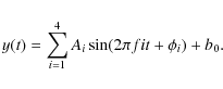 |
(2) |
This form of signal provides a better description of an eclipsing binary light curve, e.g., compared to a single sine fit. Even though the spectral peak corresponding to the orbital period (or half the orbital period) might not be significant, the periodic signal including the higher harmonics can easily be significant in that case. Furthermore, using this method, there is no need to estimate an amplitude S/N of the identified spectral peaks. Making those estimates can be ambiguous, certainly when done in an automated way. Indeed, the noise level in the amplitude spectrum is usually estimated by averaging the spectrum over a frequency interval without any significant peaks. Choosing such an interval in an automated way is not obvious and may lead to improper estimates of the noise level.
![\begin{figure}
\par\includegraphics[angle=-90,width=9cm,clip]{1618f2.ps} %
\end{figure}](/articles/aa/full_html/2009/40/aa11618-09/img30.png) |
Figure 2: The P-values of the F-test as a function of the estimated S/N. |
| Open with DEXTER | |
6.2 Interpreting the classification results
In this section, we provide guidelines for users on how to make candidate lists of their preferred objects, based on the information provided in the N3 product. First of all, if one is interested in extracting all those stars with a high confidence level of variability, the above-mentioned significance parameters can be used to select them (Fig. 2 is helpful in choosing suitable cutoff-values). Next, if the preferred object type is in the list of classes considered by the classifiers, the objects classified as such can be selected. For most of the classes (especially for the poorly defined ones), this candidate list will be contaminated by false positives, i.e., objects incorrectly assigned to the class. A supervised classification assigns every light curve to one of the pre-defined classes, even if it actually belongs to a class not included in the classification scheme, or if no clear variability is present. False positives are thus unavoidable.
The candidate lists can be cleaned further by imposing limits on the class probabilities. In general, the higher the cutoff value for the probability, the less false positives present in the resulting candidate list, and the more similar the light curves will be to the ones in the training set. We stress, however, that a low class probability (below 50%) does not necessarily mean that we are dealing with a poor candidate; for example, BCEP and DSCUT stars both show low order p-mode pulsations with a similar frequency range. Usually, the light curve information will be sufficiently discriminating to conclude that the object belongs either to the DSCUT class or to the BCEP class, but it might be difficult to decide which of the two is the real class. As a results, the light curve of a BCEP star might get similar probabilities for the BCEP and DSCUT classes, each below 0.5, but adding up to a value well above 0.5. In these cases, it is useful to have a look at the second and even the third most probable classes, and their corresponding probabilities. It is very important, in light of the BCEP-DSCUT case, to stress here that the MSBN membership probabilities basically reflect the knowledge about the relative prevalences (the prior probabilities) of the different variability classes implicit in the training set. In other words, a 50% class probability in both BCEP and DSCUT categories for a target reflects that the number of training examples of each class in the neighbourhood of the target parameters is equal. Unfortunately, it is extremely difficult (and sometimes even undesirable) to reflect the real prior probabilities in the training set. These probabilities change as a function of the age and metallicity of the environment and are, in any case, very difficult to determine. Empirically, any derived prior probability will be biased by the detection limit of the experiment, and low S/N signals will systematically be underrepresented in these estimates. Furthermore, it is sometimes convenient to overrepresent unlikely classes in the training set in order to improve detectability of rare objects (although this can also be accomplished by using tailored loss matrices to penalise unwanted misclassifications during the training of the classifiers). In any case, the ongoing improvement of the training set necessarily involves correctly determining these prior probabilities and is the subject of ongoing investigation in the framework of the Gaia and CoRoT projects (Sarro et al. 2009).
![\begin{figure}
\par\includegraphics[width=14.5cm,clip]{1618f3.ps}
\end{figure}](/articles/aa/full_html/2009/40/aa11618-09/img31.png) |
Figure 3: Examples of pulsating stars in eclipsing binary systems. In these cases, the variability due to the pulsations dominates the variability due to the eclipses, hence determines the class assignments. The light curves are classified by the MSBN classifier (from top to bottom) as belonging to the BE, DSCUT, SPB, and DSCUT categories, respectively. The original N2 level light curve is shown, together with a phase plot after detrending, made with the dominant detected frequency (given below the plot). Part of the light curves of the first three objects have been measured in oversampling mode (32 s integrations). Measurements are not averaged out during oversampling, hence the higher scatter visible in those parts of the light curves. |
| Open with DEXTER | |
We list the classification results for all objects, also for non-variable objects. Of course, if an object does not show any variability, the classification results should be disregarded (since we did not include a class of ``constant'' stars). The reason we prefer to also list the results for non-variables is twofold: first, we have to calculate all the light curve parameters anyway, because the current classifiers require a fixed number of attributes. Second, simulations have shown that noisy light curves of eclipsing binaries can still be classified correctly, even though the most common variability tests would tend to disregard the light curve as non-variable. Some of the light curve parameters typical of eclipsing binaries are less sensitive to the noise level, and they allow for a correct identification even at low S/N. In general, of course, the classification results for light curves of non-variables are not to be trusted.
Some variables actually belong to two (or even more) variability classes. Take for example a pulsating star in an eclipsing binary system: the system as a whole belongs to the eclipsing binary category, while the pulsating component might be, e.g., an SPB or a DSCUT type. How are these kinds of light curves classified? Currently, we do not have separate classes for these ``mixed'' objects. It would be difficult to define such classes, since several combinations of pulsating stars in binary systems are possible. We also do not have enough example light curves available yet to be able to define such new classes. With the current version of the classifiers, these objects will be classified as a pulsating star or an eclipsing binary, depending on the relative strength of both phenomena in the light curve. To illustrate this, Fig. 3 shows good examples of pulsating stars in binary systems. Here, the pulsations dominate the eclipses, in the sense that the highest peaks in the frequency spectrum are related to the pulsations and not to the binary orbit (remember, we only use the 3 most dominant frequencies in the spectrum). These objects are therefore not classified as eclipsing binaries, but as belonging to one of the pulsating star categories. The reverse situation, in which the highest peaks in the spectrum relate to the binary orbit, is also possible. In this case, the ``mixed'' object will be classified as an eclipsing binary. In some situations, the dominant frequency might be a pulsation frequency, while the second frequency is related to the orbit. If this orbital frequency happens to be within the range of typical pulsation frequencies of the type of pulsator in the binary system, the object can be classified as the pulsator type. If, on the other hand, the orbital frequency is far outside this range, the object will probably not be classified as pulsator type. It will also not be classified as an eclipsing binary, since most of the typical characteristics of ``pure'' eclipsing binaries in the training set relate to the first frequency and its harmonics. Hence, in this situation, the outcome of the classification is unpredictable. We cannot avoid this with the current versions of the classifiers, but research continues to detect such special cases more robustly.
7 Classification results
We present the classification results for the first four measured exoplanet fields. Since there are so many lightcurves (39 659), we obviously cannot give a detailed description for each object separately. We present an overview of the results per run in terms of numbers of detected variables and the fractions of objects assigned to every class. Light curves and phase plots of some of the best candidates are shown.
7.1 Number of variables
Since the CoRoT data are unprecedented in terms of photometric precision and time sampling, it is interesting to see how many stars appear to be variable through the eyes of CoRoT. We do point out that the sample of stars is not random. Indeed, as the main goal was to search for planets, supergiants and giants were avoided as much as possible in the target selection; i.e., the sample is heavily biased towards main-sequence stars.
We used the three frequencies and their corresponding significance parameters, resulting from the light curve analysis, to obtain estimates of the number of variables. These estimates have to be treated with caution, since, at this stage, almost all of the light curves show variability due to instrumental effects. Fortunately, most of this instrumental variability is systematic and the corresponding spectral signatures are confined to certain frequency regions in the amplitude spectrum. We were thus able to distinguish reasonably well between real (intrinsic to the observed object) and instrumental variability by avoiding spectral peaks situated in the contaminated regions. As a drawback, spectral peaks in these regions related to real variability were missed. This means that we underestimated the real number of variable light curves.
We already avoided frequencies related to the satellite orbit during the light curve analysis procedure, and also the lowest-frequency end of the spectrum. Plots of the values for f1, f2, and f3 reveal that low-frequency peaks are still selected. For selecting candidate variables, we only accepted frequency values above a certain threshold
![]() and with a corresponding significance parameter below a threshold
and with a corresponding significance parameter below a threshold
![]() .
If at least one of the three frequencies detected in the light curve fulfilled both criteria, the star was accepted as being variable. It was difficult to decide on the best value for both thresholds, providing the most reliable estimate of the number of variables. We therefore list numbers for a few combinations of these parameters, in order of increasing stringency: (
.
If at least one of the three frequencies detected in the light curve fulfilled both criteria, the star was accepted as being variable. It was difficult to decide on the best value for both thresholds, providing the most reliable estimate of the number of variables. We therefore list numbers for a few combinations of these parameters, in order of increasing stringency: (
![]() ,
0.2), (0.1 d-1, 0.1), (0.2 d-1, 0.2), and (0.2 d-1, 0.1) . Table 4 lists the resulting percentages of selected light curves for every observing run. We see that more than 40% of the stars are variable at some level if we allow periodicities up to 10 days.
,
0.2), (0.1 d-1, 0.1), (0.2 d-1, 0.2), and (0.2 d-1, 0.1) . Table 4 lists the resulting percentages of selected light curves for every observing run. We see that more than 40% of the stars are variable at some level if we allow periodicities up to 10 days.
Table 4:
Fraction of light curves in every run, fulfilling the criteria
![]() and
and
![]() for at least one of the 3 fi's, for four combinations of the thresholds
for at least one of the 3 fi's, for four combinations of the thresholds
![]() and
and
![]() .
.
7.2 Class populations
Complete classification results for the four observing runs, obtained with the MSBN and the GM classifiers, are presented in Tables 5 to 8. The GM classifier takes less classes into account than does the MSBN classifier. For example the SPDS and SXPHE classes could not be taken into account because there were not enough training instances for the GM classifier (see Paper I). Also, some classes were left out on purpose even though sufficient training examples are available for them. It concerns the classes WR, TTAU, XB, HAEBE, FUORI, and LBV. These are poorly defined on the basis of light curve information alone, because their variability can be very irregular. Moreover, such stars were avoided in the target selection, as explained above. Including them in the GM classification scheme increases the number of misclassifications.
To improve the GM classification performance for eclipsing binaries, we artificially split this class up into two subclasses, namely ECLF and ECLP. This subdivision is not based on any astrophysical differences between the objects, but is more a numerical trick to increase the number of correct classifications for this special class of variables. The ECLF subclass contains eclipsing binaries having f1/f2=2, and the ECLP subclass contains eclipsing binaries having phdiff12 = ![]() /2, phdiff13 =
/2, phdiff13 = ![]() ,
and phdiff14 =
,
and phdiff14 = ![]() /2. Most prototypical light curves of eclipsing binaries fulfil both criteria; e.g., they have both the characteristic frequency ratio and phase differences. The subdivision allows correct classification for the light curves of binaries fulfilling only one of the two criteria.
/2. Most prototypical light curves of eclipsing binaries fulfil both criteria; e.g., they have both the characteristic frequency ratio and phase differences. The subdivision allows correct classification for the light curves of binaries fulfilling only one of the two criteria.
The numbers of objects per class are obtained by counting all objects having the respective classcode as the most probable one and having a corresponding class probability classprob1
![]() .
For the MSBN classifier, numbers are listed for 3 different cutoff values
.
For the MSBN classifier, numbers are listed for 3 different cutoff values
![]() :
0.0, 0.5, and 0.7. The same probability cutoff values are used in the tables listing the GM results, but there we provide additional tables, obtained by imposing different restrictions on the Mahalanobis distance to the class centres. The precise meaning of this quantity is explained in Paper I, to which we refer for details. In short, it is a multi-dimensional generalisation of the one-dimensional statistical or standard distance (e.g. distance to the mean value of a Gaussian in terms of
:
0.0, 0.5, and 0.7. The same probability cutoff values are used in the tables listing the GM results, but there we provide additional tables, obtained by imposing different restrictions on the Mahalanobis distance to the class centres. The precise meaning of this quantity is explained in Paper I, to which we refer for details. In short, it is a multi-dimensional generalisation of the one-dimensional statistical or standard distance (e.g. distance to the mean value of a Gaussian in terms of ![]() ). It can be used effectively to reject objects that are unlikely to belong to the class (large distance to the class centres), even if the relative probability for that class is high.
). It can be used effectively to reject objects that are unlikely to belong to the class (large distance to the class centres), even if the relative probability for that class is high.
When looking at the first columns in Tables 5 and 6 (no restrictions on probability or Mahalanobis distance), one notices that a few out of the total set of considered classes seem to be strongly overpopulated (lots of light curves having the highest probability of belonging to these classes). These will typically be the poorly defined classes (wide spread in parameter space), such as PVSG, BE, CP, and LBV. As already mentioned in Sect. 6.2, most of these classifications will be false positives. Light curves with instrumental artifacts and light curves which do not fit the properties of the other classes also end up in these overpopulated classes. We tend to call these the ``trash'' classes, but we stress that also some potentially interesting objects, not belonging to any of the pre-defined classes, or objects having a mixed nature (e.g. pulsating stars in eclipsing binary systems) can end up here.
7.2.1 Eclipsing binaries and ellipsoidal variables
Irrespective of the observed region on the sky, we should always find a number of binaries: eclipsing binaries and ellipsoidal variables. This is reflected in the classification results, obtained with both classifiers. Most eclipsing binary candidates have a high probability of belonging to the ECL class and imposing stronger limits on the class probability does not alter the candidate lists much. Since eclipsing binary light curves are very different from those of pulsating variables, they are generally well separated. This translates into high relative class probabilities. The fractions we find are in the range ![]() ,
depending on the observed field. The largest fractions are found for IRa01 and SRc01, even though the time series have a shorter total time span. Assuming that the total fraction of detectable binaries is more or less the same for these observed fields, this can probably be attributed to instrumental artifacts. Light curves of longer duration have a higher chance of being influenced by instrumental variability. This is confirmed by visual inspection of a large fraction of LRa01 light curves. Some are misclassified by the presence of large discontinuities caused by cosmic-ray hits (introducing spurious peaks at low frequencies in the amplitude spectrum). Figure 4 shows some good examples of eclipsing binary light curves, correctly identified by the CVC.
,
depending on the observed field. The largest fractions are found for IRa01 and SRc01, even though the time series have a shorter total time span. Assuming that the total fraction of detectable binaries is more or less the same for these observed fields, this can probably be attributed to instrumental artifacts. Light curves of longer duration have a higher chance of being influenced by instrumental variability. This is confirmed by visual inspection of a large fraction of LRa01 light curves. Some are misclassified by the presence of large discontinuities caused by cosmic-ray hits (introducing spurious peaks at low frequencies in the amplitude spectrum). Figure 4 shows some good examples of eclipsing binary light curves, correctly identified by the CVC.
Table 5: Overview of the classification results obtained with the MSBN classifier, for each observing run, using 3 different cutoff values for the highest class probability p = classprob1.
Table 6: Same as Table 5, but now obtained with the GM classifier, with no restriction on the Mahalanobis distance to the class centre.
Table 7: Same as Table 6, but now with a cutoff value of 2.0 for the Mahalanobis distance to the class centre.
Table 8: Same as Table 6, but now with a cutoff value of 1.0 for the Mahalanobis distance to the class centre.
![\begin{figure}
\par\includegraphics[width=16cm,clip]{1618f4.ps}
\end{figure}](/articles/aa/full_html/2009/40/aa11618-09/img38.png) |
Figure 4: Some examples of eclipsing binary light curves detected with the CVC. The original N2 level light curve is shown, together with a phase plot after detrending, made with the orbital frequency (given below the plot). |
| Open with DEXTER | |
![\begin{figure}
\par\includegraphics[width=15.2cm,clip]{1618f5.ps} %
\end{figure}](/articles/aa/full_html/2009/40/aa11618-09/img39.png) |
Figure 5: Some examples of classical monoperiodic pulsators detected with the CVC in the LRc01 dataset. From top to bottom: RRab-type pulsator, RRab-type pulsator showing the Blazhko effect, RRd-type (double-mode) pulsator, and a Cepheid type pulsator. The original N2 level light curve is shown, together with a phase plot after detrending, made with the dominant pulsation frequency (given below the plot). |
| Open with DEXTER | |
7.2.2 Monoperiodic pulsators
As already emphasised, the selection of the CoRoT exoplanet observation fields is biased towards cool main-sequence stars, such that we do not expect to find many classical radial pulsators. This is indeed confirmed by the CVC classification results. These are the classes of variables best recognised by the classifiers, as shown in Papers I and II. The chance of missing them is very small, even with some discontinuities in the light curves, since these pulsators have large amplitudes compared to the order of magnitude of typical discontinuities. Some examples of the few classical pulsators we could detect are shown in Fig. 5, among them an RR-Lyrae star with a very clear Blazhko-effect (see Blazhko 1907), a double-mode RR-Lyrae, and a Cepheid pulsator. The number of detected classical Cepheids is very small, but possibly some low-amplitude Cepheids are present. Candidate low-amplitude Cepheids end up in the LAPV class. As can be seen from Tables 5 to 8, this class is well-populated for every observing run. At most a minor fraction of these variables are expected to be candidate low-amplitude Cepheids, since super giant stars have been avoided as much as possible in the target selection procedure. The large majority of the variables assigned to this class are most likely stars with variability due to rotation. Rotation can produce light curves that are difficult to distinguish from the typical skew-symmetric Cepheid light curves, if no other than CoRoT light curve information is available. Spectral information is needed and light curves with a longer total time span, to see whether the detected periods remain stable over time. Some of the rotationally modulated light curves have shorter periods than those of typical Cepheids, others have bumps or dips that are not typical of Cepheids either. Those objects can thus be distinguished by using the periods, the ratios of the different harmonic amplitudes, and their phase-differences. We are currently investigating whether this can be done in an automated way, with the aim of including a subclass of rotational variables.
It is clear that the CoRoT sample of variable stars is indeed heavily biased and completely different from, e.g., the HIPPARCOS or OGLE II sample (see Paper II and Sarro et al. 2009). In the latter, the classical radial pulsators (evolved stars) are represented very well and constitute a major fraction of the detected variable stars (especially in the OGLE case), while they are almost completely absent in the CoRoT sample. As discussed in the next section, the situation is exactly the opposite for the multiperiodic pulsators, but CoRoTs detection capabilities are a major factor there.
7.2.3 Multiperiodic pulsators
We find many more candidate multiperiodic (non-radial) pulsators in comparison with the number of monoperiodic pulsators. Part of this is again explained by the criteria used to select the CoRoT observing fields and the bias towards main-sequence stars. The main reason, however, is the high photometric precision and continuous time sampling of CoRoT. In general, multiperiodic non-radial pulsators tend to have lower amplitudes than the classical radial pulsators and are thus more difficult to detect. CoRoT allows us to explore the low-amplitude variability in a much better way, due to the low noise levels and the clean spectral window function. Furthermore, the dense time sampling of the CoRoT light curves allows much higher pulsation frequencies to be detected than most ground-based surveys are able to. Figure 6 illustrates that a major fraction of the detected variables have very low amplitudes of variation. In this figure, we plotted the fraction of objects having significant variability, and with an amplitude amp11 below a certain threshold, as a function of this threshold value. The variability criterion we used here is analogous to the one described in Sect. 7.1. Objects were taken to be variable if
![]() d-1 and
d-1 and
![]() .
The steep rise of the resulting curve at low amplitude thresholds is evident and shows that the number of detectable variables is strongly increasing with increasing amplitude detection level. A typical large-scale ground-based survey fails to detect all the small-amplitude variables at mmag level.
.
The steep rise of the resulting curve at low amplitude thresholds is evident and shows that the number of detectable variables is strongly increasing with increasing amplitude detection level. A typical large-scale ground-based survey fails to detect all the small-amplitude variables at mmag level.
![\begin{figure}
\par\includegraphics[angle=-90,width=9cm,clip]{1618f6.ps} %
\end{figure}](/articles/aa/full_html/2009/40/aa11618-09/img40.png) |
Figure 6:
Fraction of objects in the IRa01 with
|
| Open with DEXTER | |
Figure 7 shows some clear examples of candidate non-radial pulsators: ![]() -Scuti,
-Scuti, ![]() -Doradus,
-Doradus, ![]() -Cephei, and SPB candidates, respectively. Both the
-Cephei, and SPB candidates, respectively. Both the ![]() -Scuti and SPB classes are well-populated for every observing run: visual inspection of the highest probability candidates revealed many good candidates. There are less candidate
-Scuti and SPB classes are well-populated for every observing run: visual inspection of the highest probability candidates revealed many good candidates. There are less candidate ![]() -Doradus and
-Doradus and ![]() -Cephei stars. This is what one expects based on astrophysical grounds:
-Cephei stars. This is what one expects based on astrophysical grounds: ![]() -Cephei stars are very massive, hence less abundant. The
-Cephei stars are very massive, hence less abundant. The ![]() -Doradus stars show pulsations in the same frequency range as SPB stars, but they have lower amplitudes and thus are more difficult to detect. Also, our classification is based on parameters derived from only a single broad-band light curve. This implies that some of our SPB candidates might in fact be
-Doradus stars show pulsations in the same frequency range as SPB stars, but they have lower amplitudes and thus are more difficult to detect. Also, our classification is based on parameters derived from only a single broad-band light curve. This implies that some of our SPB candidates might in fact be ![]() -Doradus stars, since both classes show significant overlap in light curve parameter space (similar pulsation behaviour). The SPB stars are hotter, however, than
-Doradus stars, since both classes show significant overlap in light curve parameter space (similar pulsation behaviour). The SPB stars are hotter, however, than ![]() -Doradus stars, and a colour index (e.g. B-V) would significantly increase the separability of the two classes. Amongst the SPB sample, also good Be-star candidates are present. Be-stars show variability because of the presence of a circumstellar disk, but also because of pulsations. They are located in the same region of the HR diagram as
-Doradus stars, and a colour index (e.g. B-V) would significantly increase the separability of the two classes. Amongst the SPB sample, also good Be-star candidates are present. Be-stars show variability because of the presence of a circumstellar disk, but also because of pulsations. They are located in the same region of the HR diagram as ![]() -Cephei and SPB stars, explaining why they can show similar pulsation behaviour.
Spectral information is needed to distinguish between the classes: for Be-stars, photospheric Balmer line emission needs to be present at some stage.
-Cephei and SPB stars, explaining why they can show similar pulsation behaviour.
Spectral information is needed to distinguish between the classes: for Be-stars, photospheric Balmer line emission needs to be present at some stage.
Looking at the MSBN classification tables, we see that many objects are classified as SPDS (short period ![]() -Scuti). The majority of them are false positives and can be rejected by imposing limits on the class probability and the significance parameters Pf1 (rejecting non-variables or very noisy ones).
This class, whose training objects are actually rapidly oscillating Ap stars (roAp), attracts variables with high pulsation frequencies and low amplitudes. We have chosen to rename the class from ROAP to SPDS, because most of the objects assigned to it with high probability are in fact good candidate
-Scuti). The majority of them are false positives and can be rejected by imposing limits on the class probability and the significance parameters Pf1 (rejecting non-variables or very noisy ones).
This class, whose training objects are actually rapidly oscillating Ap stars (roAp), attracts variables with high pulsation frequencies and low amplitudes. We have chosen to rename the class from ROAP to SPDS, because most of the objects assigned to it with high probability are in fact good candidate ![]() -Scuti variables. The second most probable class is often DSCUT, with non-zero probability. Also, the typical pulsation frequencies of roAp stars are even higher than what can be detected with the nominal CoRoT 512 s time sampling, so we do not expect to find roAp stars.
In Fig. 8, we show two examples of objects in the IRa01 that are most likely
-Scuti variables. The second most probable class is often DSCUT, with non-zero probability. Also, the typical pulsation frequencies of roAp stars are even higher than what can be detected with the nominal CoRoT 512 s time sampling, so we do not expect to find roAp stars.
In Fig. 8, we show two examples of objects in the IRa01 that are most likely ![]() -Scuti stars. They have been classified as SPDS with high probability because of their high pulsation frequencies. The amplitude spectra clearly show several significant frequencies in the range 30-50 d-1. The amplitudes are low, but still far above the typical noise level of CoRoT, which is below 100 micromagnitude for these examples from the IRa01.
Below the amplitude spectra, phase plots made with the frequency corresponding to the highest peak in the amplitude spectra are shown. These confirm the presence of multiperiodic variability.
-Scuti stars. They have been classified as SPDS with high probability because of their high pulsation frequencies. The amplitude spectra clearly show several significant frequencies in the range 30-50 d-1. The amplitudes are low, but still far above the typical noise level of CoRoT, which is below 100 micromagnitude for these examples from the IRa01.
Below the amplitude spectra, phase plots made with the frequency corresponding to the highest peak in the amplitude spectra are shown. These confirm the presence of multiperiodic variability.
![\begin{figure}
\par\includegraphics[width=15cm,clip]{1618f7.ps}
\end{figure}](/articles/aa/full_html/2009/40/aa11618-09/img41.png) |
Figure 7:
Some examples of multiperiodic pulsators detected with the CVC. From top to bottom: a candidate |
| Open with DEXTER | |
![\begin{figure}
\par\includegraphics[width=15.7cm,clip]{1618f8.eps} %
\end{figure}](/articles/aa/full_html/2009/40/aa11618-09/img42.png) |
Figure 8:
Two examples of candidate short-period |
| Open with DEXTER | |
8 Conclusions
This work describes the application of the classification methodology presented in Papers I and II to the database of light curves produced in the CoRoT exoplanet programme. The methods are broadly applicable, but database-specific adaptations always have to be made to maintain optimal classification performance. This proved to be very important for the application to the CoRoT data, since the data quality is much better than the major fraction of the data used to construct the original training set. We described how we extended the training set by including high quality CoRoT data in an iterative way and how we adapted the light curve analysis procedure to avoid instrumental effects. Changes have been made to the classification methods themselves as well. The combination of all these adaptations led to increased classification performance.
Classification results and statistics on the number of variables are presented for the first four measured fields of the exoplanet programme of CoRoT. Conservative estimates show that up to 40% of all the light curves are variable. Irrespective of the observed field, the class statistics show that there are more multiperiodic pulsators than classical monoperiodic pulsators. This is consistent with the bias towards main-sequence stars, thanks to the CoRoT target selection procedure, which makes the sample of variable stars very different from those obtained from large-scale surveys such as HIPPARCOS and OGLE. It is also strongly related to the high photometric precision and the continuous time sampling of CoRoT, allowing us to detect more small-amplitude variables. A significant fraction of (quasi-)monoperiodic variables with low amplitudes is present in every field. Most likely, the majority of them are
rotationally modulated variables, and possibly, some of them are low-amplitude Cepheids. We have yet to investigate if there are statistically significant differences in the class populations from field to field.
Some representative light curves and phase plots for the different classes are shown, illustrating the high quality of the CoRoT data and the capabilities of our classifiers. The classification results and the derived light curve parameters are made publicly available for every observing run (CVC N3 product). Guidelines are given to use these results for the creation of candidate lists with different levels of contamination (or false positives). We strongly advise users of the classification results to read these guidelines in advance, since they illustrate both the strengths and limitations of the current methods. We stress that this is a statistical method and that we can never guarantee ![]() correct classifications. Individual misclassifications will always occur, and their incidence strongly depends on the variability class considered (as can be seen from the confusion matrices presented in Paper I). Our goal is of course to keep the number of misclassifications as low as possible, and we continue to work on that.
correct classifications. Individual misclassifications will always occur, and their incidence strongly depends on the variability class considered (as can be seen from the confusion matrices presented in Paper I). Our goal is of course to keep the number of misclassifications as low as possible, and we continue to work on that.
The same methods will be applied to the data from the other observed fields in the exoplanet programme, some of them yet to be measured. We also plan to upgrade the results for the first four fields presented here on the longer term. Since the database is still growing, we will be able to extend the training set with CoRoT data, and possibly include new classes and/or subclasses. Other planned improvements include a better and fully automated treatment of discontinuities in the light curves, with the goal of avoiding misclassifications related herewith. Since the total number of stars in the CoRoT exoplanet database will be more than twice the number we have already analysed in this work, we expect to find many more candidate variables. Apart from the eclipsing binaries, which are omnipresent, it is difficult to say at this stage how many more candidates we will find for each category. CoRoT is observing different regions of the galactic centre and anti-centre, whose stellar populations can vary a lot. The bias towards main-sequence stars still holds, however, and the fraction of classical pulsators will remain small. The correction for instrumental effects will have the biggest influence on low-amplitude variables, such as ![]() Doradus,
Doradus, ![]() Scuti, and eclipsing binaries with shallow eclipses. Their numbers are expected to increase significantly (by several percents, relatively) after improvement of our methods. Based on astrophysical arguments, we do not expect to find many good candidate
Scuti, and eclipsing binaries with shallow eclipses. Their numbers are expected to increase significantly (by several percents, relatively) after improvement of our methods. Based on astrophysical arguments, we do not expect to find many good candidate ![]() Cephei stars in the CoRoT fields. Not only are those massive stars less abundant, most stars in CoRoT's exoplanet fields are also intrinsically too faint to be of the
Cephei stars in the CoRoT fields. Not only are those massive stars less abundant, most stars in CoRoT's exoplanet fields are also intrinsically too faint to be of the ![]() Cephei type, given their visual magnitudes in combination with distance estimates.
Cephei type, given their visual magnitudes in combination with distance estimates.
This work has focused on the supervised classification of light curves, a very efficient and fast method for identifying objects of an already known variability type. As mentioned in Sect. 6.2, this method has some shortcomings as well. For example, it is difficult to detect new types of objects, since the classes have to be pre-defined. Therefore, to explore the full potential of the CoRoT database, we are also applying unsupervised classification methods to the data (better known as clustering techniques). The methodology and the results will be published in a forthcoming paper (Sarro et al. 2009). Finally, spectroscopic observation time with the ESO VLT/FLAMES instrument was obtained to observe the variables we identified in the IRa01 and LRa01 CoRoT fields. The resulting spectra will help reveal and confirm the truly variable nature of the objects we classified using only light curve information, so they will be important to evaluate the classification results. Since spectra of several thousands of objects will become available, it will be possible to investigate how classification attributes derived from these spectra (e.g. equivalent line widths) can improve the classification performance, both for supervised and unsupervised methods. An extended classifier that also uses spectroscopic attributes could be used and provided by e.g the VSOP project (variable star one-shot project, Dall et al. 2007).
Acknowledgements
This work is made possible thanks to support from the Belgian PRODEX programme under grant PEA C90199 (CoRoT Mission Data Exploitation II), and from the research Council of Leuven University under grant GOA/2008/04. J.D. wishes to thank R. Alonso, P.-Y. Chabaud, and T. Fenouillet for their help with software issues and preparation of the CoRoT data during his stay at LAM (Laboratoire d'Astrophysique de Marseille). L.M.S., M.L., and E.S. wishes to acknowledge the support of the Spanish MICINN through the project AyA2005-04286 (Spanish Virtual Observatory).
References
- Blazhko, S. 1907, Astr. Nachr., 175, 325 [NASA ADS] [CrossRef] (In the text)
- Breger, M., Stich, J., Garrido, R., et al. 1993, A&A, 271, 482 [NASA ADS]
- Buchler, J. R., Wood, P. R., Keller, S., & Soszynski, I. 2005, ApJ, 631, L151 [NASA ADS] [CrossRef] (In the text)
- Dall, T. H., Foellmi, C., Pritchard, J., et al. 2007, A&A, 470, 1201 [NASA ADS] [CrossRef] [EDP Sciences] (In the text)
- Debosscher, J., Sarro, L. M., Aerts, C., et al. 2007, A&A, 475, 1159 [NASA ADS] [CrossRef] [EDP Sciences] (In the text)
- Kuschnig, R., Weiss, W. W., Gruber, R., Bely, P. Y., & Jenkner, H. 1997, A&A, 328, 544 [NASA ADS]
- Lomb, N. R. 1976, Ap&SS, 39, 447 [NASA ADS] [CrossRef]
- Sarro, L. M., Debosscher, J., López, M., & Aerts, C. 2009a, A&A, 494, 739 [NASA ADS] [CrossRef] [EDP Sciences] (In the text)
- Sarro, L. M., Debosscher, J., Aerts, C., & López, M. 2009b, A&A, 506, 535 [CrossRef] [EDP Sciences]
- Scargle, J. D. 1982, ApJ, 263, 835 [NASA ADS] [CrossRef]
Footnotes
- ... fields
- The CoRoT space mission, launched on 27 December 2006, has been developed and is operated by the CNES, with the contribution of Austria, Belgium, Brazil , ESA, Germany, and Spain.
- ...
- The full classification results will be only available in electronic form at the CDS via anonymous ftp to cdsarc.u-strasbg.fr (130.79.128.5) or via http://cdsweb.u-strasbg.fr/cgi-bin/qcat?J/A+A/506/519
All Tables
Table 1: Basic properties of the data, coming from the first 4 exoplanet fields, having a 512 s nominal sampling time.
Table 2: Variability classes whose definition stars have been extended/replaced with CoRoT data, and the number of definition CoRoT light curves used.
Table 3: The different variability classes considered by the CVC and our abbreviations.
Table 4:
Fraction of light curves in every run, fulfilling the criteria
![]() and
and
![]() for at least one of the 3 fi's, for four combinations of the thresholds
for at least one of the 3 fi's, for four combinations of the thresholds
![]() and
and
![]() .
.
Table 5: Overview of the classification results obtained with the MSBN classifier, for each observing run, using 3 different cutoff values for the highest class probability p = classprob1.
Table 6: Same as Table 5, but now obtained with the GM classifier, with no restriction on the Mahalanobis distance to the class centre.
Table 7: Same as Table 6, but now with a cutoff value of 2.0 for the Mahalanobis distance to the class centre.
Table 8: Same as Table 6, but now with a cutoff value of 1.0 for the Mahalanobis distance to the class centre.
All Figures
| |
Figure 1: Some CoRoT light curves of low-amplitude periodic variables, measured in the IRa01. The original N2 level light curve is shown with a phase plot after detrending, made with the dominant detected frequency (given below the plot). |
| Open with DEXTER | |
| In the text | |
| |
Figure 2: The P-values of the F-test as a function of the estimated S/N. |
| Open with DEXTER | |
| In the text | |
| |
Figure 3: Examples of pulsating stars in eclipsing binary systems. In these cases, the variability due to the pulsations dominates the variability due to the eclipses, hence determines the class assignments. The light curves are classified by the MSBN classifier (from top to bottom) as belonging to the BE, DSCUT, SPB, and DSCUT categories, respectively. The original N2 level light curve is shown, together with a phase plot after detrending, made with the dominant detected frequency (given below the plot). Part of the light curves of the first three objects have been measured in oversampling mode (32 s integrations). Measurements are not averaged out during oversampling, hence the higher scatter visible in those parts of the light curves. |
| Open with DEXTER | |
| In the text | |
| |
Figure 4: Some examples of eclipsing binary light curves detected with the CVC. The original N2 level light curve is shown, together with a phase plot after detrending, made with the orbital frequency (given below the plot). |
| Open with DEXTER | |
| In the text | |
| |
Figure 5: Some examples of classical monoperiodic pulsators detected with the CVC in the LRc01 dataset. From top to bottom: RRab-type pulsator, RRab-type pulsator showing the Blazhko effect, RRd-type (double-mode) pulsator, and a Cepheid type pulsator. The original N2 level light curve is shown, together with a phase plot after detrending, made with the dominant pulsation frequency (given below the plot). |
| Open with DEXTER | |
| In the text | |
| |
Figure 6:
Fraction of objects in the IRa01 with
|
| Open with DEXTER | |
| In the text | |
| |
Figure 7:
Some examples of multiperiodic pulsators detected with the CVC. From top to bottom: a candidate |
| Open with DEXTER | |
| In the text | |
| |
Figure 8:
Two examples of candidate short-period |
| Open with DEXTER | |
| In the text | |
Copyright ESO 2009
Current usage metrics show cumulative count of Article Views (full-text article views including HTML views, PDF and ePub downloads, according to the available data) and Abstracts Views on Vision4Press platform.
Data correspond to usage on the plateform after 2015. The current usage metrics is available 48-96 hours after online publication and is updated daily on week days.
Initial download of the metrics may take a while.