| Issue |
A&A
Volume 505, Number 3, October III 2009
|
|
|---|---|---|
| Page(s) | 1255 - 1264 | |
| Section | The Sun | |
| DOI | https://doi.org/10.1051/0004-6361/200912368 | |
| Published online | 27 August 2009 | |
EUV filter responses to plasma emission for the nonthermal  -distributions
J. Dudík1 - A. Kulinová1,2 - E. Dzifcáková1,2 - M. Karlický2
1 - Department of Astronomy, Physics of the Earth, and Meteorology, Faculty of Mathematics, Physics and Informatics, Comenius University, Mlynská Dolina F2, 842 48 Bratislava, Slovak Republic
2 -
Astronomical Institute of the Academy of Sciences of the Czech Republic, Fricova 298, 251 65 Ondrejov, Czech Republic
Received 22 April 2009 / Accepted 16 July 2009
Abstract
The responses to plasma emission of the TRACE EUV filters are computed by integrating their spectral responses over the synthetic spectra obtained from the CHIANTI database. The filter responses to emission are functions of temperature, electron density, and the assumed electron distribution function. It is shown here that, for the nonthermal ![]() -distributions, the resulting responses to emission are more broadly dependent on T, and their maxima are flatter than for the Maxwellian electron distribution. The positions of the maxima can also be shifted. Filter reponses to T are density-dependent as well. The influence of the nonthermal
-distributions, the resulting responses to emission are more broadly dependent on T, and their maxima are flatter than for the Maxwellian electron distribution. The positions of the maxima can also be shifted. Filter reponses to T are density-dependent as well. The influence of the nonthermal ![]() -distributions on the diagnostics of T from the observations in all three EUV filters is discussed.
-distributions on the diagnostics of T from the observations in all three EUV filters is discussed.
Key words: Sun: corona - hydrodynamics - Sun: UV radiation - stars: coronae
1 Introduction
One of the fundamental assumptions in the physics of the solar corona is that the particle distribution function is Maxwellian. This assumption automatically requires that the solar coronal plasma is collisionally dominated. However, under the physical conditions normally present in the corona, this assumption may not be accurate. Strong gradients of temperature or density at low plasma densities may lead to departures from the Maxwellian distribution. The distribution function formed under these condition is characterized by a higher number of particles in the high-energy tail of the distribution in comparison with the Maxwellian one (e.g., Owocki & Scudder 1983; Shoub 1983; Scudder & Olbert 1979b; Dufton et al. 1984; Roussel-Dupré 1980; Scudder 1992; Scudder & Olbert 1979a; Pinfield et al. 1999; Ljepojevic & MacNiece 1988).
Such a distribution with an enhanced high-energy tail would lead to observable effects, since in the optically thin solar corona the ionization and excitation processes are driven by collisions. Dufton et al. (1984) and Pinfield et al. (1999) concluded that such nonthermal distributions could explain the observed Si III line intensities. Owocki & Scudder (1983) suggested that the assumption of the nonthermal, two-parametric ![]() -distribution, characterized by parameters
-distribution, characterized by parameters ![]() and T with the power-law tail (Vasyliunas 1968), could explain the observed O VII/O VIII line ratios. The
and T with the power-law tail (Vasyliunas 1968), could explain the observed O VII/O VIII line ratios. The ![]() -distribution is also able to explain the observed velocity distribution in the solar wind (Zouganelis 2008), and it yields a better fit to the data than either one or the sum of two Maxwellian distributions (Maksimovic et al. 1997). The connection between the
-distribution is also able to explain the observed velocity distribution in the solar wind (Zouganelis 2008), and it yields a better fit to the data than either one or the sum of two Maxwellian distributions (Maksimovic et al. 1997). The connection between the ![]() -distributions and the acceleration of the solar wind have been studied by Zouganelis et al. (2005,2004). Collier (2004) argues that, in the dynamic systems where energy is not conserved but the order of magnitude of the particle energy is, the
-distributions and the acceleration of the solar wind have been studied by Zouganelis et al. (2005,2004). Collier (2004) argues that, in the dynamic systems where energy is not conserved but the order of magnitude of the particle energy is, the ![]() -distribution is maximizing the specific entropy. I.e., if the heating of the solar corona is dynamical (e.g., Patsourakos & Klimchuk 2005; Parker 1988; Sarkar & Walsh 2008; Ugarte-Urra et al. 2006; Brooks et al. 2008), the particle distribution in the corona is given by a
-distribution is maximizing the specific entropy. I.e., if the heating of the solar corona is dynamical (e.g., Patsourakos & Klimchuk 2005; Parker 1988; Sarkar & Walsh 2008; Ugarte-Urra et al. 2006; Brooks et al. 2008), the particle distribution in the corona is given by a ![]() -distribution. The formation of the
-distribution. The formation of the
![]() -distributions by self-consistent plasma processes has been studied by Yoon et al. (2000) and Rhee et al. (2006). Leubner (2004) point out that particle distribution can be described by the sum of two
-distributions by self-consistent plasma processes has been studied by Yoon et al. (2000) and Rhee et al. (2006). Leubner (2004) point out that particle distribution can be described by the sum of two ![]() -distributions, one with a positive and one with a negative value of parameter
-distributions, one with a positive and one with a negative value of parameter ![]() in natural equilibrium state within the generalized entropy concept (e.g., Leubner 2002; Tsallis 1998). Vocks et al. (2008) studied the formation of the suprathermal electron distribution in connection to the
in natural equilibrium state within the generalized entropy concept (e.g., Leubner 2002; Tsallis 1998). Vocks et al. (2008) studied the formation of the suprathermal electron distribution in connection to the ![]() -distributions in the closed coronal loop geometry.
-distributions in the closed coronal loop geometry.
The influence of the ![]() -distributions on the ionization equilibrium, excitation
equilibrium, or line intensities of the ions commonly observed in the transition region or coronal spectrum have been studied by Dzifcáková (2000); Anderson et al. (1996); Dzifcáková (1992,2006a,2002), and Dzifcáková & Kulinová (2003). Dzifcáková (2006a) report that the Fe VIII - XV line intensities computed under the assumption of
-distributions on the ionization equilibrium, excitation
equilibrium, or line intensities of the ions commonly observed in the transition region or coronal spectrum have been studied by Dzifcáková (2000); Anderson et al. (1996); Dzifcáková (1992,2006a,2002), and Dzifcáková & Kulinová (2003). Dzifcáková (2006a) report that the Fe VIII - XV line intensities computed under the assumption of ![]() -distributions can differ significantly from those obtained under the assumption of Maxwellian distribution. Since some of these lines are prominent in the spectral domains covered by the commonly used set of EUV filters, the influence of the
-distributions can differ significantly from those obtained under the assumption of Maxwellian distribution. Since some of these lines are prominent in the spectral domains covered by the commonly used set of EUV filters, the influence of the ![]() -distributions on the filter responses to plasma emission of these filters needs to be evaluated, because the signal detected by EUV filters is a function of intensities of lines within their spectral windows, and also because the intensities of these lines can be changed by
-distributions on the filter responses to plasma emission of these filters needs to be evaluated, because the signal detected by EUV filters is a function of intensities of lines within their spectral windows, and also because the intensities of these lines can be changed by ![]() -distributions. In addition, the ratios of filter responses to T are commonly used in the temperature diagnostic of the coronal plasma (e.g., Noglik & Walsh 2007; Chae et al. 2002). Also, the filter responses to T are the key element in modeling the emission distribution of active regions (e.g., Warren & Winebarger 2006; Lundquist et al. 2008b; Gontikakis et al. 2008; Mok et al. 2005; Winebarger et al. 2008; Alexander et al. 1997; Warren & Winebarger 2007; Lundquist et al. 2008a), or the entire corona (e.g., Schrijver et al. 2004), which are done in an attempt to constrain the properties of the coronal heating (see e.g. Aschwanden 2005; or Klimchuk 2006, for a recent rewiev of the coronal heating problem). The task of evaluating the effect of nonthermal
-distributions. In addition, the ratios of filter responses to T are commonly used in the temperature diagnostic of the coronal plasma (e.g., Noglik & Walsh 2007; Chae et al. 2002). Also, the filter responses to T are the key element in modeling the emission distribution of active regions (e.g., Warren & Winebarger 2006; Lundquist et al. 2008b; Gontikakis et al. 2008; Mok et al. 2005; Winebarger et al. 2008; Alexander et al. 1997; Warren & Winebarger 2007; Lundquist et al. 2008a), or the entire corona (e.g., Schrijver et al. 2004), which are done in an attempt to constrain the properties of the coronal heating (see e.g. Aschwanden 2005; or Klimchuk 2006, for a recent rewiev of the coronal heating problem). The task of evaluating the effect of nonthermal ![]() -distributions on the filter responses to emission is carried out in this paper.
-distributions on the filter responses to emission is carried out in this paper.
This paper is organized as follows. The method used to compute the filter responses to T is described in Sect. 2, which includes the description of the ![]() -distributions (Sect. 2.1) and the computation of synthetic spectra (Sect. 2.2). Section 3 summarizes the results obtained for
-distributions (Sect. 2.1) and the computation of synthetic spectra (Sect. 2.2). Section 3 summarizes the results obtained for ![]() -distributions and compares them to the results for the Maxwellian distribution. Conclusions are given in Sect. 4.
-distributions and compares them to the results for the Maxwellian distribution. Conclusions are given in Sect. 4.
2 Computational method
2.1 The -distributions
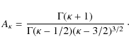
The ![]() -distribution
-distribution
![]() )
as a function of the parameter
)
as a function of the parameter ![]() and the electron kinetic energy E is defined as (e.g. Owocki & Scudder 1983)
and the electron kinetic energy E is defined as (e.g. Owocki & Scudder 1983)
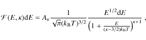
where
The limit case of
It must be noted that the representation of the parameter T as temperature is valid only in terms of the mean energy of the distribution,
![]() ,
which is the same for both the Maxwellian and
,
which is the same for both the Maxwellian and ![]() -distributions. If the particle distribution function is isotropic, it immediately follows (e.g., Dzifcáková & Mason 2008; Dzifcáková 2006a) that
-distributions. If the particle distribution function is isotropic, it immediately follows (e.g., Dzifcáková & Mason 2008; Dzifcáková 2006a) that
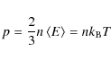
for both Maxwellian and
2.2 Line intensities and synthetic spectra
The emissivity
![]() in a line with wavelength
in a line with wavelength
![]() corresponding to the transition between levels i and j, i > j, in the ion k of the element x, is given by
corresponding to the transition between levels i and j, i > j, in the ion k of the element x, is given by
where Aij is the Einstein coefficient for the spontaneous emission, h the Planck constant, c the speed of light, ni the density of the emitting ions,
Since the solar corona is an optically thin medium, the observed intensity I of the line with
![]() is given by the integral of its emissivity along the observer's line of sight l:
is given by the integral of its emissivity along the observer's line of sight l:
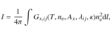
where
The commonly used EUV spectral windows located in the neighborhood of the wavelengths of 171 Å, 195 Å and 284 Å are dominated by lines of various Fe ions. The situation is illustrated in Fig. 1 for Maxwellian and ![]() -distribution with
-distribution with
![]() .
The synthetic spectra presented in Fig. 1 were computed using the CHIANTI atomic database, version 5.2 (Dere et al. 1997; Landi et al. 2006), which has been modified by Dzifcáková (2006b) for computing synthetic spectra for nonthermal distributions. The full-widths at half-maximum, FWHM, of the emission lines displayed in Fig. 1, have been set to the thermal FWHM for the corresponding values of T.
.
The synthetic spectra presented in Fig. 1 were computed using the CHIANTI atomic database, version 5.2 (Dere et al. 1997; Landi et al. 2006), which has been modified by Dzifcáková (2006b) for computing synthetic spectra for nonthermal distributions. The full-widths at half-maximum, FWHM, of the emission lines displayed in Fig. 1, have been set to the thermal FWHM for the corresponding values of T.
The synthetic spectra for the Maxwellian distribution were computed using the sun_coronal_ext.abund abundance file based on the data in Feldman et al. (1992), Grevesse & Sauval (1998) and Landi et al. (2002). The ionization equilibrium was computed using the ionization fraction file mazotta_etal_ext.ioneq based on the work of Mazzotta et al. (1998) and Landini & Monsignori Fossi (1991).
Modification of the CHIANTI database for the nonthermal ![]() -distributions (Dzifcáková 2006b) utilizes the ionization equilibrium for Fe ions obtained by Dzifcáková (1992,2002). In addition, Dzifcáková (2000) has shown that the deviation in excitation rates for the
-distributions (Dzifcáková 2006b) utilizes the ionization equilibrium for Fe ions obtained by Dzifcáková (1992,2002). In addition, Dzifcáková (2000) has shown that the deviation in excitation rates for the ![]() -distributions from the Maxwellian case are sufficient enough to affect the line intensities. Finally, Dzifcáková (2006a) computed the Fe line intensities by incorporating the changes in both ionization and excitation. The synthetic spectra for the
-distributions from the Maxwellian case are sufficient enough to affect the line intensities. Finally, Dzifcáková (2006a) computed the Fe line intensities by incorporating the changes in both ionization and excitation. The synthetic spectra for the ![]() -distributions computed with this modified CHIANTI database use the same sun_coronal_ext.abund abundance file as the computation for the Maxwellian distribution. The computation of the ionization equilibrium is based on the works of Dzifcáková (2002), Dzifcáková & Kulinová (2003) and Dzifcáková (2006b). It must be noted that this ionization equilibrium contains data only for C, N, O, Ne, Mg, Al, Si, S, Ar, Ca, Fe, and Ni. This is important because the observations in the TRACE 284 Å filter can contain leakage from the two He II 303.8 Å lines (Handy et al. 1999), formed at log
-distributions computed with this modified CHIANTI database use the same sun_coronal_ext.abund abundance file as the computation for the Maxwellian distribution. The computation of the ionization equilibrium is based on the works of Dzifcáková (2002), Dzifcáková & Kulinová (2003) and Dzifcáková (2006b). It must be noted that this ionization equilibrium contains data only for C, N, O, Ne, Mg, Al, Si, S, Ar, Ca, Fe, and Ni. This is important because the observations in the TRACE 284 Å filter can contain leakage from the two He II 303.8 Å lines (Handy et al. 1999), formed at log
![]() .
These lines are not present in the synthetic spectra calculated for the
.
These lines are not present in the synthetic spectra calculated for the ![]() -distributions. They do not appear in Fig. 1 bottom left, because their intensities are negligible at log
-distributions. They do not appear in Fig. 1 bottom left, because their intensities are negligible at log
![]() .
The synthetic spectra computed for the nonthermal
.
The synthetic spectra computed for the nonthermal ![]() -distributions do not contain contributions from the continuum either.
-distributions do not contain contributions from the continuum either.
![\begin{figure}
\par\mbox{\includegraphics[height=7.7cm]{12368f1a.eps} \includegr...
...m]{12368f1e.eps} \includegraphics[height=7.7cm]{12368f1f.eps} }
\end{figure}](/articles/aa/full_html/2009/39/aa12368-09/img38.png) |
Figure 1:
Isothermal synthetic spectra computed using CHIANTI database (version 5.2) for the Maxwellian distribution ( left column) and
|
| Open with DEXTER | |
2.3 EUV filter responses
The signal F registered through an EUV filter is an integral of the filter spectral
response
![]() times the spectrum, which is characterized by the electron density
times the spectrum, which is characterized by the electron density ![]() and parameters T and
and parameters T and ![]() ,
over the spectral window of the given filter and the line of sight l:
,
over the spectral window of the given filter and the line of sight l:
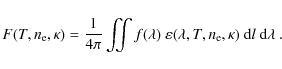
The units of the
where G represents the sum of the contribution functions of all lines of the considered elements plus the continuum. The standard value of EM in the CHIANTI database is 1027 cm-5. The computed function
From all presently available EUV imaging instruments, i.e., SOHO/EIT (Delaboudinière et al. 1996), TRACE (Handy et al. 1999), and STEREO/EUVI (Wuelser et al. 2004), we chose TRACE to demonstrate the influence of the ![]() -distributions on the filter responses to emission. This selection is based on TRACE having the highest spatial resolution. The spectral responses
-distributions on the filter responses to emission. This selection is based on TRACE having the highest spatial resolution. The spectral responses
![]() of the three TRACE EUV ``ao'' filters (171, 195, and 284 Å, Handy et al. 1999) are overlaid on the computed synthetic spectra in Fig. 1. These spectral responses were computed using the trace_euv_resp.pro routine of the SolarSoft environment (Freeland & Handy 1998) running with the Interactive Data Language (IDL).
of the three TRACE EUV ``ao'' filters (171, 195, and 284 Å, Handy et al. 1999) are overlaid on the computed synthetic spectra in Fig. 1. These spectral responses were computed using the trace_euv_resp.pro routine of the SolarSoft environment (Freeland & Handy 1998) running with the Interactive Data Language (IDL).
3 Results
![\begin{figure}
\par\includegraphics[height=7.7cm]{12368f2.eps}
\end{figure}](/articles/aa/full_html/2009/39/aa12368-09/img45.png) |
Figure 2:
Effect of the ``missing'' He II emission on the TRACE 284 Å filter response to T for
|
| Open with DEXTER | |
3.1 The effect of continuum and lines of missing ions in the case of the Maxwellian distribution
The aim of this section is to evaluate the effect of the continuum and emission from the ions missing in the ionization equilibria computed by Dzifcáková (2006b). Of course, this effect can only be evaluated in the known case, i.e. for the Maxwellian distribution. To do that, the filter responses to emission for the Maxwellian distribution with continuum, without continuum, and without continuum but including only those ions for which the nonthermal ionization equilibria exists, were computed in the temperature range of log
To study the effect of the continuum, the cases with and without continuum were compared to each other. It was found that the effect of the continuum is generally less than 3% for all three filters in the range of log
![]() .
This range of T contains the dominant maxima of all three filters. Outside of this range the filter responses of the 171 and 195 Å filters for the assumed Maxwellian distribution are usually negligible because of the absence of strong emission lines, and the contribution to the filter responses is mostly from the continuum.
.
This range of T contains the dominant maxima of all three filters. Outside of this range the filter responses of the 171 and 195 Å filters for the assumed Maxwellian distribution are usually negligible because of the absence of strong emission lines, and the contribution to the filter responses is mostly from the continuum.
To evaluate the effect of missing ions, the cases without continuum with all ions were compared to those with only the ions with known nonthermal ionization equilibrium. The result is that the effect of the missing ions is generally negligible (i.e., <![]() ), except in two cases:
), except in two cases: ![]() 1.7% error due to two K XIV lines formed at 195 and 196 Å at
log
1.7% error due to two K XIV lines formed at 195 and 196 Å at
log
![]() ,
and the He II emission at 303.8 Å formed at a wider range of temperatures, with maximum at log
,
and the He II emission at 303.8 Å formed at a wider range of temperatures, with maximum at log
![]() for the Maxwellian distribution. The He II emission is responsible for the appearance of the smallest peak in the TRACE 284 Å filter response to T (Fig. 2).
for the Maxwellian distribution. The He II emission is responsible for the appearance of the smallest peak in the TRACE 284 Å filter response to T (Fig. 2).
![\begin{figure}
\par\includegraphics[height=7.8cm]{12368f3a.eps}
\includegraphi...
...m]{12368f3b.eps}
\includegraphics[height=7.8cm]{12368f3c.eps}
\par\end{figure}](/articles/aa/full_html/2009/39/aa12368-09/img53.png) |
Figure 3:
TRACE EUV filter responses to T for the Maxwellian and |
| Open with DEXTER | |
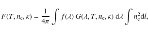
3.2 TRACE EUV filter responses to emission for the Maxwellian and -distributions
Following the approach outlined in Sect. 2.3, the TRACE EUV filter responses to emission for the Maxwellian and ![]() -distributions with
-distributions with
![]() ,
3 and 5 were computed for the assumed value of
,
3 and 5 were computed for the assumed value of
![]() cm-3. The range of T is the same as in the previous section, i.e. log
cm-3. The range of T is the same as in the previous section, i.e. log
![]() ,
with the step of
,
with the step of
![]() .
The results are displayed in Fig. 3.
.
The results are displayed in Fig. 3.
The TRACE EUV filter responses to emission for ![]() -distributions are significantly different from those for the Maxwellian distribution. In general, their peaks are lower and significantly wider for all three filters. The decrease of the peak heights of the filter response to emission functions is expected, since it comes directly from the intensity behavior with
-distributions are significantly different from those for the Maxwellian distribution. In general, their peaks are lower and significantly wider for all three filters. The decrease of the peak heights of the filter response to emission functions is expected, since it comes directly from the intensity behavior with ![]() of the contributing lines (e.g., compare left column of
Fig. 1 with the right column of the same figure). Such behavior is reported for all DEMs implemented in CHIANTI (Dzifcáková 2006a). The peak heights
of the contributing lines (e.g., compare left column of
Fig. 1 with the right column of the same figure). Such behavior is reported for all DEMs implemented in CHIANTI (Dzifcáková 2006a). The peak heights
![]() of the filter responses to emission, together with the corresponding values of
of the filter responses to emission, together with the corresponding values of
![]() for Maxwellian (
for Maxwellian (
![]() )
and
)
and ![]() -distributions, are listed in Table 1.
-distributions, are listed in Table 1.
To quantify the width of the
![]() peaks, we determined the location of their half-maxima T1 and T2, defined by the relation
peaks, we determined the location of their half-maxima T1 and T2, defined by the relation
![]() ;
;
![]() .
The FWHM of the filter response to T is then defined as
.
The FWHM of the filter response to T is then defined as
![]() .
The advantage of this quantity is that it only characterizes the primary maximum (the strongest peak), since the secondary peaks for the 195 and 284 Å filters are sufficiently low.
.
The advantage of this quantity is that it only characterizes the primary maximum (the strongest peak), since the secondary peaks for the 195 and 284 Å filters are sufficiently low.
Another possibility of quantifying the width of the
![]() is to compute its equivalent width W, i.e. the area of the function F divided by
is to compute its equivalent width W, i.e. the area of the function F divided by
![]() .
This quantity is for the logarithmic sampling in T defined as
.
This quantity is for the logarithmic sampling in T defined as
 |
(8) |
The equivalent width takes the entire area of the filter response to emission into account, including any and all secondary maxima. The values of T1, T2, FWHM, and W for each TRACE EUV filter and also values of
Table 1:
TRACE EUV filter characteristics for
![]() cm-3.
cm-3.
As the distribution function changes from a Maxwellian one to the ![]() -distribution, noticeable shifts in the
-distribution, noticeable shifts in the
![]() location occur. The shifts are toward higher values of T in the
location occur. The shifts are toward higher values of T in the
![]() case and to the slightly lower values for
case and to the slightly lower values for
![]() and 5. This is caused by changes in the ionization and excitation equilibrium. Generally, the ionization peaks are shifted to higher T values (Figs. 3-5 of Dzifcáková 2002). The excitation peaks are generally shifted to lower values of T, but the details differ from line to line. This comes from dependence of the excitation rates on
and 5. This is caused by changes in the ionization and excitation equilibrium. Generally, the ionization peaks are shifted to higher T values (Figs. 3-5 of Dzifcáková 2002). The excitation peaks are generally shifted to lower values of T, but the details differ from line to line. This comes from dependence of the excitation rates on ![]() ,
the
,
the
![]() ratio, and the colissional cross-section, which is also dependent on Eij (Dzifcáková 2006a). Dzifcáková (2006a) studied the dependence on
ratio, and the colissional cross-section, which is also dependent on Eij (Dzifcáková 2006a). Dzifcáková (2006a) studied the dependence on ![]() and T of the electron excitation rates and relative level population of the Fe XV 284.2 Å line
(Figs. 4 and 5 therein). With decreasing
and T of the electron excitation rates and relative level population of the Fe XV 284.2 Å line
(Figs. 4 and 5 therein). With decreasing ![]() ,
the excitation rates decrease for values
of T higher or corresponding to the maximum abundance of the Fe XV ion, while it increases for lower values of T. The relative level population shows similar behavior.
,
the excitation rates decrease for values
of T higher or corresponding to the maximum abundance of the Fe XV ion, while it increases for lower values of T. The relative level population shows similar behavior.
For
![]() ,
the ionization equilibrium shift effect seems to be more significant, while the changes due to the excitation equilibrium are dominant for
,
the ionization equilibrium shift effect seems to be more significant, while the changes due to the excitation equilibrium are dominant for
![]() and 5. It must be noted here that, for
and 5. It must be noted here that, for
![]() ,
the shift in the peak location of the 171 Å filter is expected to be small because of the small shift of the Fe X ion abundance peak. The shift in the peak locations of the 195 and 284 Å filters is expected to be greater, as suggested by Fig. 5 of Dzifcáková (2002).
,
the shift in the peak location of the 171 Å filter is expected to be small because of the small shift of the Fe X ion abundance peak. The shift in the peak locations of the 195 and 284 Å filters is expected to be greater, as suggested by Fig. 5 of Dzifcáková (2002).
3.3 The effect of electron density
Mok et al. (2005) computed the EIT filter responses to plasma emission for several values of the electron density ![]() ,
with log
,
with log
![]() (see Fig. 11 therein). The EIT filter responses to emission showed weak dependence
on
(see Fig. 11 therein). The EIT filter responses to emission showed weak dependence
on ![]() .
To study the possible dependence of the TRACE EUV filter responses to emission on the electron density
.
To study the possible dependence of the TRACE EUV filter responses to emission on the electron density ![]() ,
they were recomputed in the ranges of log
,
they were recomputed in the ranges of log
![]() and log
and log
![]() with the step of
with the step of
![]() and
and
![]() .
The range in
.
The range in ![]() is shifted to higher values than those used by Mok et al. (2005). It has been chosen so that it accomodates structures commonly observed in the EUV filters, most notably coronal holes with densities of 108 cm-3 (e.g., Fludra et al. 1999; Chiuderi Drago et al. 1999), active region coronal loops (including flare loops), whose densities are on the order of 109 cm-3 (e.g., Ugarte-Urra et al. 2005; Aschwanden et al. 1999; Noglik et al. 2009; Aschwanden et al. 2000,2008) ranging from several times of 108 cm-3 to several times of 1010 cm-3 (e.g., Landi & Landini 2004; Schmelz et al. 2009; Varady et al. 2000; Tripathi et al. 2009; Brosius et al. 1996; Gallagher et al. 2001; Landi et al. 2003) or up to 1011 cm-3 (e.g., Phillips et al. 2005).
is shifted to higher values than those used by Mok et al. (2005). It has been chosen so that it accomodates structures commonly observed in the EUV filters, most notably coronal holes with densities of 108 cm-3 (e.g., Fludra et al. 1999; Chiuderi Drago et al. 1999), active region coronal loops (including flare loops), whose densities are on the order of 109 cm-3 (e.g., Ugarte-Urra et al. 2005; Aschwanden et al. 1999; Noglik et al. 2009; Aschwanden et al. 2000,2008) ranging from several times of 108 cm-3 to several times of 1010 cm-3 (e.g., Landi & Landini 2004; Schmelz et al. 2009; Varady et al. 2000; Tripathi et al. 2009; Brosius et al. 1996; Gallagher et al. 2001; Landi et al. 2003) or up to 1011 cm-3 (e.g., Phillips et al. 2005).
The results displayed in Figs. 4 and 5 show the dependence of the
![]() functions on
functions on ![]() ,
normalized to the value of
,
normalized to the value of
![]() cm-5. The most notable changes in primary or secondary maxima of all three filters are around typical coronal values of log
cm-5. The most notable changes in primary or secondary maxima of all three filters are around typical coronal values of log
![]() .
The total changes in the values of primary and secondary maxima between log
.
The total changes in the values of primary and secondary maxima between log
![]() and 13 are summarized in Table 2.
and 13 are summarized in Table 2.
If emission measure is held constant, the spectral lines can respond in two different ways to the changes in the electron density: the line intensity can either decrease or increase with increasing ![]() at constant EM. The intensities of lines with the highest contribution to the filter responses to emission present in the spectrum at log
at constant EM. The intensities of lines with the highest contribution to the filter responses to emission present in the spectrum at log
![]() (Fig. 1), i.e. lines Fe IX 171.1 Å,
Fe X 174.5 Å, Fe XII 195.1 Å, and Fe XV 284.2 Å (for log
10(T) = 6.0, 6.2, and 6.3, respectively) decrease with increasing
(Fig. 1), i.e. lines Fe IX 171.1 Å,
Fe X 174.5 Å, Fe XII 195.1 Å, and Fe XV 284.2 Å (for log
10(T) = 6.0, 6.2, and 6.3, respectively) decrease with increasing ![]() at constant EM. The decrease in primary maxima of the
at constant EM. The decrease in primary maxima of the
![]() ,
caused by these lines, is combated up to a degree by the lines whose intensities increase with increasing
,
caused by these lines, is combated up to a degree by the lines whose intensities increase with increasing ![]() at constant EM. For
at constant EM. For
![]() cm-3, intensities of some of these lines are comparable to (e.g. Fe X 175.3 Å) or even higher (Fe XIII 196.5 Å) than the intensities of lines dominant at
cm-3, intensities of some of these lines are comparable to (e.g. Fe X 175.3 Å) or even higher (Fe XIII 196.5 Å) than the intensities of lines dominant at
![]() cm-3. In contrast to this, the primary maximum of the 284 Å filter is constituted practically only by the Fe XV 284.2 Å line, because the contribution from any other line is less than an order of magnitude smaller.
cm-3. In contrast to this, the primary maximum of the 284 Å filter is constituted practically only by the Fe XV 284.2 Å line, because the contribution from any other line is less than an order of magnitude smaller.
The situation is different for the secondary maxima of the 195 and 284 Å filters. The secondary maximum of the 195 Å filter, located at log
![]() ,
is dominated by the two O V lines (192.8 and 192.9 Å). Intensities of these two O V lines increase with increasing
,
is dominated by the two O V lines (192.8 and 192.9 Å). Intensities of these two O V lines increase with increasing ![]() at constant EM, resulting in the noticeable increase in the secondary maximum (Fig. 4). If the deviation from the Maxwellian distribution is rather strong (
at constant EM, resulting in the noticeable increase in the secondary maximum (Fig. 4). If the deviation from the Maxwellian distribution is rather strong (
![]() ), the contribution from the two Fe VIII lines (194.7 and 196.0 Å) also takes on significance. The situation is similar, but more complicated for the secondary maximum of the 284 Å filter, which is constituted by a multitude of Si and Mg lines. Intensities of some of them decrease (Si VII 275.4 Å, Mg VII 277.0 and two 278.4 Å lines), while intensities of other lines increase (Si VIII 276.9 and 277.1 Å,
Mg VII 280.7 Å) with increasing
), the contribution from the two Fe VIII lines (194.7 and 196.0 Å) also takes on significance. The situation is similar, but more complicated for the secondary maximum of the 284 Å filter, which is constituted by a multitude of Si and Mg lines. Intensities of some of them decrease (Si VII 275.4 Å, Mg VII 277.0 and two 278.4 Å lines), while intensities of other lines increase (Si VIII 276.9 and 277.1 Å,
Mg VII 280.7 Å) with increasing ![]() and constant EM. The combination of both effects results in an increase in the secondary maximum with
and constant EM. The combination of both effects results in an increase in the secondary maximum with ![]() .
For
.
For
![]() ,
the contribution from several Al IX and Si IX lines located at
,
the contribution from several Al IX and Si IX lines located at
![]() Å increases significantly. The dependence of these lines on T actually causes the disappearance of the secondary maximum for
Å increases significantly. The dependence of these lines on T actually causes the disappearance of the secondary maximum for
![]() (Fig. 3 bottom and Fig. 5 top right).
(Fig. 3 bottom and Fig. 5 top right).
 |
Figure 4:
TRACE 171 and 195 Å filter responses to emission
|
| Open with DEXTER | |
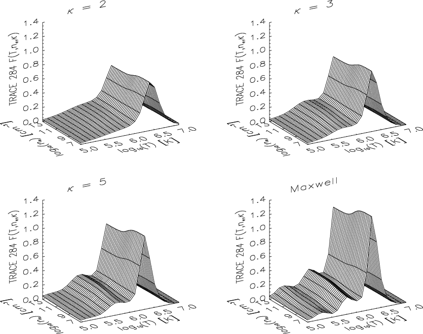 |
Figure 5: Same as in Fig. 4, but for the TRACE 284 Å filter. |
| Open with DEXTER | |
Table 2:
Ratios of
![]() cm
cm
![]() cm
cm
![]() for the primary and secondary maxima.
for the primary and secondary maxima.
![\begin{figure}
\par\mbox{\includegraphics[height=7.4cm]{12368f6a.eps} \includegraphics[height=7.4cm]{12368f6b.eps} }
\end{figure}](/articles/aa/full_html/2009/39/aa12368-09/img77.png) |
Figure 6:
TRACE filter ratios computed under the assumption of
|
| Open with DEXTER | |
![\begin{figure}
\par\includegraphics[width=11.5cm,clip]{12368f7.eps}
\end{figure}](/articles/aa/full_html/2009/39/aa12368-09/img78.png) |
Figure 7: Color-color diagram for the diagnostic of parameter T. |
| Open with DEXTER | |
3.4 Diagnostic of T and
from filter ratios
In this section we evaluate the possibility of diagnosing T and ![]() from the ratios of signals measured in the TRACE EUV filters. The 195/171 and 284/195 filter ratios are plotted in Fig. 6, from which it is clear that these ratios are strongly dependent on the value of
from the ratios of signals measured in the TRACE EUV filters. The 195/171 and 284/195 filter ratios are plotted in Fig. 6, from which it is clear that these ratios are strongly dependent on the value of ![]() .
However, even with the knowledge of
.
However, even with the knowledge of ![]() ,
a single filter ratio cannot yield a unique result, since the ratio is not a monotonical function of T, but instead exhibits one or more peaks (Fig. 6). This is a well known property of the EUV filters and the assumed Maxwellian distribution (see e.g. Fig. 1 of Chae et al. 2002; Fig. 1 of Noglik & Walsh 2007; Fig. 2 bottom of Aschwanden et al. 2008; or Fig. 6 of Schmelz et al. 2009). The TRACE EUV filter ratios are also dependent on
,
a single filter ratio cannot yield a unique result, since the ratio is not a monotonical function of T, but instead exhibits one or more peaks (Fig. 6). This is a well known property of the EUV filters and the assumed Maxwellian distribution (see e.g. Fig. 1 of Chae et al. 2002; Fig. 1 of Noglik & Walsh 2007; Fig. 2 bottom of Aschwanden et al. 2008; or Fig. 6 of Schmelz et al. 2009). The TRACE EUV filter ratios are also dependent on ![]() .
In the X-ray spectral domain, where observations in several filters are usually available, a combination of them could be used to determine the temperature unambiguously (e.g., Reale et al. 2007), if the Maxwellian distribution is assumed. In the EUV part of the spectrum, only three filters are available.
.
In the X-ray spectral domain, where observations in several filters are usually available, a combination of them could be used to determine the temperature unambiguously (e.g., Reale et al. 2007), if the Maxwellian distribution is assumed. In the EUV part of the spectrum, only three filters are available.
To deal with the inherent ambiguity problem of a single filter ratio, Chae et al. (2002) proposes the color-color diagram method. This method uses the fact that the dependence of the 195/171 filter ratio on the 284/195 filter ratio constitutes a spatial color-color curve, which can be utilized to determine temperature of the observed EUV structures under the assumption that the time of observation is identical in all three filters and also that these structures are isothermal (see e.g. Schmelz et al. 2009; and Mulu-Moore et al. 2009, for a study of the isothermality of the coronal loops). Chae et al. (2002) used this color-color diagram method further to determine the temperature of three observed coronal loops, EUV moss, and EUV jet. They reported that the temperature of a coronal loop observed in all three TRACE EUV filters determined by this color-color diagram method could differ from the temperature obtained from the two single filter ratios (0.24 MK vs. 1.2 and 1.8 MK, Table 1 therein).
The color-color diagram for the TRACE EUV filter responses to emission computed for
![]() ,
3, and 5 and a Maxwellian distribution with
,
3, and 5 and a Maxwellian distribution with
![]() cm-3
is shown in Fig. 7 for the range of log
cm-3
is shown in Fig. 7 for the range of log
![]() .
The color-color diagram is strongly dependent on the value of
.
The color-color diagram is strongly dependent on the value of ![]() ,
as the location of points with the same value of T can be very different for different distributions.
,
as the location of points with the same value of T can be very different for different distributions.
The largest discrepancies in determining T can occur at log
![]() and log
and log
![]() ,
where the similar ratio of EUV filters gives unequal values of T for Maxwellian and
,
where the similar ratio of EUV filters gives unequal values of T for Maxwellian and ![]() -distributions with different
-distributions with different ![]() .
Thus, there are a few regions in the color-color diagram where the diagnostic of T is impossible without a priori knowledge of
.
Thus, there are a few regions in the color-color diagram where the diagnostic of T is impossible without a priori knowledge of ![]() .
On the other hand, the differences between color-color curves for Maxwellian and
.
On the other hand, the differences between color-color curves for Maxwellian and ![]() -distributions are large for
-distributions are large for
![]() (Fig. 7) and in principle they could allow the determination of
(Fig. 7) and in principle they could allow the determination of ![]() and T for given
and T for given ![]() ,
if the filter ratios are known with sufficient precission.
,
if the filter ratios are known with sufficient precission.
The situation is complicated by the dependence of the
![]() on electron density
on electron density ![]() .
This dependence changes the shape of the color-color curves mainly for log
.
This dependence changes the shape of the color-color curves mainly for log
![]() (Fig. 8). For different values of
(Fig. 8). For different values of ![]() ,
the curves corresponding to different
,
the curves corresponding to different ![]() can touch or even overlap. This severely complicates the possibility of diagnostic T and
can touch or even overlap. This severely complicates the possibility of diagnostic T and ![]() without the a priori knowledge of
without the a priori knowledge of ![]() .
.
We thus suggest using the spectroscopic measurements to properly diagnose the values of T, ![]() ,
and
,
and ![]() .
The possibilities of a diagnostic of the plasma parameters from the Fe lines observed by the HINODE/EIS and SPIRIT instruments were thoroughly studied and discussed in Dzifcáková & Kulinová (2009). They concluded that the diagnostic of the
.
The possibilities of a diagnostic of the plasma parameters from the Fe lines observed by the HINODE/EIS and SPIRIT instruments were thoroughly studied and discussed in Dzifcáková & Kulinová (2009). They concluded that the diagnostic of the ![]() -distribution in the solar corona is possible, even though the ratios of the coronal Fe line intensities are in general strongly dependent on
-distribution in the solar corona is possible, even though the ratios of the coronal Fe line intensities are in general strongly dependent on ![]() .
However, the
line ratios used for density diagnostics are only affected by the nonthermal distribution a little. The value of
.
However, the
line ratios used for density diagnostics are only affected by the nonthermal distribution a little. The value of ![]() for the known electron density can be diagnosed from the line ratios of different Fe ions more easily than from the line ratios of a single Fe ion. They recommended using this nonthermal diagnostic for bright homogeneous structures (e.g., single bright loops) to reduce errors from plasma inhomogeneities.
for the known electron density can be diagnosed from the line ratios of different Fe ions more easily than from the line ratios of a single Fe ion. They recommended using this nonthermal diagnostic for bright homogeneous structures (e.g., single bright loops) to reduce errors from plasma inhomogeneities.
4 Conclusions
We computed the filter responses to emission
![]() for the
for the ![]() -distributions with the considered values of the parameter
-distributions with the considered values of the parameter
![]() ,
3, and 5. The results are compared to the results for the Maxwellian distribution. We have shown that the filter responses to T are much broader for the
,
3, and 5. The results are compared to the results for the Maxwellian distribution. We have shown that the filter responses to T are much broader for the ![]() -distributions than for the Maxwellian distribution. The peak values are increasingly lower with a decreasing value of
-distributions than for the Maxwellian distribution. The peak values are increasingly lower with a decreasing value of ![]() ,
i.e., increasing deviations from the Maxwellian distribution. These differences are caused by the changes in the EUV emission spectrum of the coronal plasma for the
,
i.e., increasing deviations from the Maxwellian distribution. These differences are caused by the changes in the EUV emission spectrum of the coronal plasma for the ![]() -distributions. Moreover, the peak locations of the filter responses to T can be shifted due to the changes in ionization and excitation.
-distributions. Moreover, the peak locations of the filter responses to T can be shifted due to the changes in ionization and excitation.
The filter responses to plasma emission for the nonthermal ![]() -distributions of the free electrons were computed without the contribution of the continuum and even of some lines, notably the He II 303.8 Å lines present in the TRACE 284 Å channel. The absence of the He II lines comes from the present unavailability of the ionization and excitation data for these lines for the
-distributions of the free electrons were computed without the contribution of the continuum and even of some lines, notably the He II 303.8 Å lines present in the TRACE 284 Å channel. The absence of the He II lines comes from the present unavailability of the ionization and excitation data for these lines for the ![]() -distributions. The absence of the continuum is justified, since its contribution is usually negligible and the spectrum is dominated by emission lines.
-distributions. The absence of the continuum is justified, since its contribution is usually negligible and the spectrum is dominated by emission lines.
![\begin{figure}
\par\includegraphics[height=8.6cm]{12368f8.eps}
\end{figure}](/articles/aa/full_html/2009/39/aa12368-09/img83.png) |
Figure 8:
Dependence of the color-color diagram on the electron density |
| Open with DEXTER | |
We also studied the density dependence of the filter responses to emission
![]() .
It was found that, if the emission measure is assumed to be constant, all primary maxima decrease with increasing
.
It was found that, if the emission measure is assumed to be constant, all primary maxima decrease with increasing ![]() .
The dependence of the filter response to emission on electron density is again caused by the behavior of spectral lines in spectrum. The intensity of the strongest lines present in the spectral windows of the TRACE EUV filters decrease with increasing electron density and constant EM. The spectrum also contains lines with reversed behavior, but the effect of these lines is generally less than the effect of the strongest lines for T corresponding to the primary peaks. The situation is reversed for secondary peaks.
.
The dependence of the filter response to emission on electron density is again caused by the behavior of spectral lines in spectrum. The intensity of the strongest lines present in the spectral windows of the TRACE EUV filters decrease with increasing electron density and constant EM. The spectrum also contains lines with reversed behavior, but the effect of these lines is generally less than the effect of the strongest lines for T corresponding to the primary peaks. The situation is reversed for secondary peaks.
The possibility of the diagnostic of T utilizing the measurements in all three TRACE EUV filters and the color-color diagram method is complicated by different location of points with the same value of T for different distributions. There are regions in color-color diagram where it is impossible to diagnose T without the knowledge of the value of parameter ![]() .
On the other hand, there is a small region of the color-color diagram where the diagnostic of
.
On the other hand, there is a small region of the color-color diagram where the diagnostic of ![]() and T is in principle possible, if the electron density is known. The dependence of the color-color curves on electron density complicates the diagnostic possibilities.
and T is in principle possible, if the electron density is known. The dependence of the color-color curves on electron density complicates the diagnostic possibilities.
Acknowledgements
The authors are indebted to E. Landi for helpful discussions regarding the preparation of the .ioneq files for the CHIANTI software package. This work was supported by the Scientific Grant Agency, VEGA, Slovakia, Grant No. 1/0069/08, Grant IAA300030701 of the Grant Agency of the Academy of Sciences of the Czech Republic, Grant No. 205/09/1705 of the Grant Agency of the Czech Republic, and the Comenius University Grants No. 414/2008 and 398/2009. J.D. wishes to express his thanks for the hospitality provided by the staff of the Astronomical Institute of the Czech Republic. CHIANTI is a collaborative project involving the NRL (USA), RAL (UK), MSSL (UK), the Universities of Florence (Italy) and Cambridge (UK), and George Mason University (USA). The Solar and Heliospheric Observatory (SOHO) is a project of international cooperation between ESA and NASA. The Transition Region and Coronal Explorer (TRACE) is a mission of the Stanford-Lockheed Institute for Space Research, and part of the NASA Small Explorer program. The SOlar TErrestrial RElations Observatory (STEREO) mission is a part of the NASA Solar Terrestrial Probes program. HINODE is a Japanese mission developed and launched by ISAS/JAXA, with NAOJ as domestic partner and NASA and STFC (UK) as international partners. It is operated by these agencies in co-operation with ESA and NSC (Norway).
References
- Alexander, D., Gary, G. A., & Thompson, B. J. 1997, ASP Conf. Ser., 155, 100 [NASA ADS]
- Anderson, S. W., Raymond, J. C., & van Ballegooijen, A. 1996, ApJ, 457, 939 [NASA ADS] [CrossRef]
- Aschwanden, M. J. 2005, Physics of the Solar Corona: An Introduction (Chichester, United Kingdom: Praxis Publishing Ltd.) (In the text)
- Aschwanden, M. J., Newmark, J. S., Delaboudinière, J.-P., et al. 1999, ApJ, 515, 842 [NASA ADS] [CrossRef]
- Aschwanden, M. J., Alexander, D., Hulburt, N., et al. 2000, ApJ, 531, 1129 [NASA ADS] [CrossRef]
- Aschwanden, M. J., Nitta, N. V., Wuelser, J.-P., & Lemen J. R. 2008, ApJ, 680, 1477 [NASA ADS] [CrossRef]
- Brooks, D. H., Ugarte-Urra, I., & Warren, H. P. 2008, ApJ, 689, 77 [NASA ADS] [CrossRef]
- Brosius, J. W., Davila, J. M., Thomas, R. J., & Monsignori-Fossi, B. C. 1997, ApJS, 106, 143 [NASA ADS] [CrossRef]
- Chae, J., Park, Y.-D., Moon, Y.-J., Wang, H., & Yun, H. S. 2002, ApJ, 567, 159 [NASA ADS] [CrossRef]
- Chiuderi Drago, F., Landi, E., Fludra, A., & Kerdraon, A. 1999, A&A, 348, 261 [NASA ADS]
- Collier, M. R. 2004, Adv. Space Res., 33, 2108 [NASA ADS] [CrossRef] (In the text)
- Delaboudinière, J.-P., Artzner, G. E., & Brunaud, J. 1996, Sol. Phys., 162, 291 [NASA ADS] [CrossRef] (In the text)
- Dere, K. P., Landi, E., Mason, H. E., et al. 1997, A&AS, 125, 149 [NASA ADS] [CrossRef] [EDP Sciences]
- Dufton, P. L., Kingston, A. E., & Keenan, F. P. 1984 ApJ, 280, L35
- Dzifcáková, E. 1992, Sol. Phys., 140, 247 [NASA ADS] [CrossRef]
- Dzifcáková, E. 2000, Sol. Phys., 196, 113 [NASA ADS] [CrossRef]
- Dzifcáková, E. 2002, Sol. Phys., 208, 91 [NASA ADS] [CrossRef]
- Dzifcáková, E. 2006a, Sol. Phys., 234, 243 [NASA ADS] [CrossRef]
- Dzifcáková E. 2006b, in Proc. SOHO-17, 10 Years of SOHO and Beyond, ed. H. Lacoste, & L. Ouwehand, ESA SP-617, 89.1 (In the text)
- Dzifcáková, E., & Kulinová, A. 2003, Sol. Phys., 218, 41 [NASA ADS] [CrossRef] (In the text)
- Dzifcáková, E., & Kulinová, A. 2009, Sol. Phys., submitted (In the text)
- Dzifcáková, E., & Mason, H. 2008, Sol. Phys., 247, 301 [NASA ADS] [CrossRef]
- Feldman, U., Mandelbaum, P., Seely, J. L., Doschek, G. A., & Gursky, H. 1992, ApJS, 81, 387 [NASA ADS] [CrossRef] (In the text)
- Fludra, A., Del Zanna, G., Alexander, D., & Bromage, B. J. I. 1999, J. Geophys. Res., 104, 9709 [NASA ADS] [CrossRef]
- Freeland, S. N., & Handy, B. N. 1998, Sol. Phys., 182, 497 [NASA ADS] [CrossRef] (In the text)
- Gallagher, P. T., Phillips, K. J. H., Lee, J., Keenan, F. P., & Pinfield, D. J. 2001, ApJ, 558, 411 [NASA ADS] [CrossRef]
- Gontikakis, C., Contopoulos, I., & Dara, H. C. 2008, A&A, 489, 441 [NASA ADS] [CrossRef] [EDP Sciences]
- Grevesse, N., & Sauval, A. J. 1998, Space Sci. Rev., 85, 161 [NASA ADS] [CrossRef] (In the text)
- Handy, B. N., Acton, L. W., Kankelborg, C. C., et al. 1999, Sol. Phys., 187, 229 [NASA ADS] [CrossRef] (In the text)
- Klimchuk, J. A. 2006, Sol. Phys., 234, 41 [NASA ADS] [CrossRef] (In the text)
- Landi, E., & Landini, M. 2004, ApJ, 608, 1133 [NASA ADS] [CrossRef]
- Landi, E., Feldman, U., & Dere, K. P. 2002, ApJ, 139, 281 [NASA ADS] [CrossRef] (In the text)
- Landi, E., Feldman, U., Innes, D. E., & Curdt, W. 2003, ApJ, 582, 506 [NASA ADS] [CrossRef]
- Landi, E., Del Zanna, G., Dere, K. P., Mason, H. E., & Landini, M. 2006, ApJS, 162, 261 [NASA ADS] [CrossRef]
- Landini, M., & Monsignori Fossi, B. C. 1991, A&AS, 91, 183 [NASA ADS] (In the text)
- Leubner, M. P. 2002, Ap&SS, 282, 573 [NASA ADS] [CrossRef]
- Leubner, M. P. 2004, ApJ, 604, 469 [NASA ADS] [CrossRef] (In the text)
- Ljepojevic, N. N., & MacNiece, P. 1987, Sol. Phys., 117, 123 [NASA ADS] [CrossRef]
- Lundquist, L. L., Fisher, G. H., & McTiernan, J. M. 2008a, ApJS, 179, 509 [NASA ADS] [CrossRef]
- Lundquist, L. L., Fisher, G. H., Metcalf, T. R., Leka, K. D., & McTiernan, J. M. 2008b ApJ, 689, 1388
- Maksimovic, M., Pierrard, V., & Lemaire, J. F. 1997, A&A, 324, 725 [NASA ADS] (In the text)
- Mazzotta, P., Mazzitelli, G., Colafrancesco, S., & Vittorio, N. 1998, A&AS, 133, 403 [NASA ADS] [CrossRef] [EDP Sciences] (In the text)
- Mok, Y., Mikic, Z., Lionello, R., & Linker, J. A. 2005, ApJ, 621, 1098 [NASA ADS] [CrossRef]
- Mulu-Moore, F., Winebarger, A. R., Warren, H. P., & Aschwanden, M. J. 2009, BAAS, 41, 830 (In the text)
- Noglik, J. B., & Walsh, R. W. 2007, ApJ, 655, 1127 [NASA ADS] [CrossRef]
- Noglik, J. B., Walsh, R. W., & Maclean, R. C. 2009, ApJ, submitted
- Owocki, S. P., & Scudder, J. D. 1983, ApJ, 270, 758 [NASA ADS] [CrossRef]
- Parker, E. N. 1988, ApJ, 330, 474 [NASA ADS] [CrossRef]
- Patsourakos, S., & Klimchuk, J. A. 2005, ApJ, 628, 1023 [NASA ADS] [CrossRef]
- Phillips, K. J. H., Feldman, U., & Harra, L. K. 2005, ApJ, 634, 641 [NASA ADS] [CrossRef] (In the text)
- Phillips, K. J. H., Feldman, U., & Landi, E. 2008, Ultraviolet and 1.6 Spectroscopy of the Solar Atmosphere (Cambridge, United Kingdom: Cambridge University Press) (In the text)
- Pinfield, D. J., Keenan, F. P., Mathioudakis, M., et al. 1999, ApJ, 527, 1000 [NASA ADS] [CrossRef]
- Reale, F., Parenti, S., Reeves, K. K., et al. 2007, Sci., 318, 1582 [NASA ADS] [CrossRef] (In the text)
- Rhee, T., Chang-Mo, R., & Yoon, P.-H. 2006, J. Geophys. Res., 111, A09107 [CrossRef] (In the text)
- Roussel-Dupre, R. 1980, Sol. Phys., 68, 265 [NASA ADS] [CrossRef]
- Sarkar, A., & Walsh, R. W. 2008, ApJ, 683, 516 [NASA ADS] [CrossRef]
- Scudder, J. D. 1992, ApJ, 398, 319 [NASA ADS] [CrossRef]
- Scudder, J. D., & Olbert, S. 1979a, J. Geophys. Res., 84, 2755 [NASA ADS] [CrossRef]
- Scudder, J. D., & Olbert, S. 1979b, J. Geophys. Res., 84, 6603 [NASA ADS] [CrossRef]
- Shoub, E. C. 1983, ApJ, 266, 339 [NASA ADS] [CrossRef]
- Schmelz, J. T., Nasraoui, K., Rightmire, L. A., et al. 2009, ApJ, 691, 503 [NASA ADS] [CrossRef]
- Schrijver, C. J., Sandman, A. W., Aschwanden, M. J., & DeRosa, M. L. 2004, ApJ, 615, 512 [NASA ADS] [CrossRef] (In the text)
- Tripathi, D., Mason, H. E., Dwivedi, B. N., del Zanna, G., & Young, P. R. 2009, ApJ, 694, 1256 [NASA ADS] [CrossRef]
- Tsallis, C. 1998, J. Stat. Phys., 52, 479 [NASA ADS] [CrossRef]
- Ugarte-Urra, I., Doyle, J. G., Walsh, R. W., & Madjarska, M. S. 2005, A&A, 439, 351 [NASA ADS] [CrossRef] [EDP Sciences]
- Ugarte-Urra, I., Winebarger, A. R., & Warren, H. P. 2006, ApJ, 643, 1245 [NASA ADS] [CrossRef]
- Varady, M., Fludra, A., & Heinzel, P. 2000, A&A, 355, 769 [NASA ADS]
- Vasyliunas, V. M. 1968, in Proc. Physics of the Magnetosphere, ed. R. L. D. Carrovilano, & J. F. McClay, ASSL, 10, 622 (In the text)
- Vásquez, A. M., Frazin, R. A., & Kalamabadi, F. 2009, Sol. Phys., 256, 73 [NASA ADS] [CrossRef] (In the text)
- Vocks, C., Mann, G., & Rausche, G. 2008, A&A, 480, 527 [NASA ADS] [CrossRef] [EDP Sciences] (In the text)
- Warren, H. P., & Winebarger, A. R. 2006, ApJ, 645, 711 [NASA ADS] [CrossRef]
- Warren, H. P., & Winebarger, A. R. 2007, ApJ, 666, 1245 [NASA ADS] [CrossRef]
- Winebarger, A. R., Warren, H. P., & Falconer, D. 2008, ApJ, 676, 672 [NASA ADS] [CrossRef]
- Wuelser, J. P., Lemen, J. R., Tarbell, T. D., et al. 2004, Proc. Int. Soc. Opt. Eng., 5171, 111 (In the text)
- Yoon, P. H., Rhee, T., & Chang-Mo, R. 2006, J. Geophys. Res., 111, A09106 [CrossRef] (In the text)
- Zouganelis, I. 2008, J. Geophys. Res., 113, A08111 [CrossRef] (In the text)
- Zouganelis, I., Maksimovic, M., Meyer-Vernet, N., Lamy, H., & Issautier, K. 2004, ApJ, 606, 542 [NASA ADS] [CrossRef]
- Zouganelis, I., Meyer-Vernet, N., Landi, S., Maksimovic, M., & Pantellini, F. 2005, ApJ, 626, L117 [NASA ADS] [CrossRef]
All Tables
Table 1:
TRACE EUV filter characteristics for
![]() cm-3.
cm-3.
Table 2:
Ratios of
![]() cm
cm
![]() cm
cm
![]() for the primary and secondary maxima.
for the primary and secondary maxima.
All Figures
| |
Figure 1:
Isothermal synthetic spectra computed using CHIANTI database (version 5.2) for the Maxwellian distribution ( left column) and
|
| Open with DEXTER | |
| In the text | |
| |
Figure 2:
Effect of the ``missing'' He II emission on the TRACE 284 Å filter response to T for
|
| Open with DEXTER | |
| In the text | |
| |
Figure 3:
TRACE EUV filter responses to T for the Maxwellian and |
| Open with DEXTER | |
| In the text | |
| |
Figure 4:
TRACE 171 and 195 Å filter responses to emission
|
| Open with DEXTER | |
| In the text | |
| |
Figure 5: Same as in Fig. 4, but for the TRACE 284 Å filter. |
| Open with DEXTER | |
| In the text | |
| |
Figure 6:
TRACE filter ratios computed under the assumption of
|
| Open with DEXTER | |
| In the text | |
| |
Figure 7: Color-color diagram for the diagnostic of parameter T. |
| Open with DEXTER | |
| In the text | |
| |
Figure 8:
Dependence of the color-color diagram on the electron density |
| Open with DEXTER | |
| In the text | |
Copyright ESO 2009
Current usage metrics show cumulative count of Article Views (full-text article views including HTML views, PDF and ePub downloads, according to the available data) and Abstracts Views on Vision4Press platform.
Data correspond to usage on the plateform after 2015. The current usage metrics is available 48-96 hours after online publication and is updated daily on week days.
Initial download of the metrics may take a while.