| Issue |
A&A
Volume 505, Number 3, October III 2009
|
|
|---|---|---|
| Page(s) | 969 - 979 | |
| Section | Cosmology (including clusters of galaxies) | |
| DOI | https://doi.org/10.1051/0004-6361/200811459 | |
| Published online | 27 August 2009 | |
Cosmological model discrimination with weak lensing
S. Pires1 - J.-L. Starck1 - A. Amara1,2 - A. Réfrégier1 - R. Teyssier1
1 - Laboratoire AIM, CEA/DSM-CNRS-Universite Paris Diderot, IRFU/SEDI-SAP, Service d'Astrophysique, CEA Saclay, Orme des Merisiers, 91191 Gif-sur-Yvette, France
2 - Department of Physics, ETH Zürich, Wolfgang-Pauli-Strasse 16, 8093 Zürich, Switzerland
Received 2 December 2008 / Accepted 18 June 2009
Abstract
Weak gravitational lensing provides a unique way of mapping directly the dark matter in the Universe. The majority of lensing analyses use the two-point statistics of the cosmic shear field to constrain the cosmological model, a method that is affected by degeneracies, such as that between ![]() and
and
![]() which are respectively the rms of the mass fluctuations on a scale of 8 Mpc/h and the matter density parameter, both at z = 0. However, the two-point statistics only measure the Gaussian properties of the field, and the weak lensing field is non-Gaussian. It has been shown that the estimation of non-Gaussian statistics for weak lensing data can improve the constraints on cosmological parameters. In this paper, we systematically compare a wide range of non-Gaussian estimators to determine which one provides tighter constraints on the cosmological parameters. These statistical methods include skewness, kurtosis, and the higher criticism test, in several sparse representations such as wavelet and curvelet; as well as the bispectrum, peak counting, and a newly introduced statistic called wavelet peak counting (WPC). Comparisons based on sparse representations indicate that the wavelet transform is the most sensitive to non-Gaussian cosmological structures. It also appears that the most helpful statistic for non-Gaussian characterization in weak lensing mass maps is the WPC. Finally, we show that the
which are respectively the rms of the mass fluctuations on a scale of 8 Mpc/h and the matter density parameter, both at z = 0. However, the two-point statistics only measure the Gaussian properties of the field, and the weak lensing field is non-Gaussian. It has been shown that the estimation of non-Gaussian statistics for weak lensing data can improve the constraints on cosmological parameters. In this paper, we systematically compare a wide range of non-Gaussian estimators to determine which one provides tighter constraints on the cosmological parameters. These statistical methods include skewness, kurtosis, and the higher criticism test, in several sparse representations such as wavelet and curvelet; as well as the bispectrum, peak counting, and a newly introduced statistic called wavelet peak counting (WPC). Comparisons based on sparse representations indicate that the wavelet transform is the most sensitive to non-Gaussian cosmological structures. It also appears that the most helpful statistic for non-Gaussian characterization in weak lensing mass maps is the WPC. Finally, we show that the ![]() -
-
![]() degeneracy could be even better broken if the WPC estimation is performed on weak lensing mass maps filtered by the wavelet method, MRLens.
degeneracy could be even better broken if the WPC estimation is performed on weak lensing mass maps filtered by the wavelet method, MRLens.
Key words: gravitational lensing - methods: data analysis - methods: statistical - cosmological parameters - dark matter
1 Introduction
Measurements of the image distortion of background galaxies caused by large-scale structures provide a direct way to study the statistical properties of the growth of structures in the Universe. Weak gravitational lensing measures the mass and can thus be directly compared to theoretical models of structure formation. Most lensing studies use the two-point statistics of the cosmic shear field because of its potential to constrain the power spectrum of density fluctuations in the late Universe (e.g., Dahle 2006; Refregier et al. 2002; Bacon et al. 2003; Maoli et al. 2001; Massey et al. 2005). Two-point statistics measure the Gaussian properties of the field. This represents a limited amount of information since it is well known that the low redshift Universe is highly non-Gaussian on small scales. Gravitational clustering is, indeed, a non linear process and on small scales, in particular, the mass distribution is highly non-Gaussian. Consequently, using only two-point statistics to place constraints on the cosmological model provides limited insight. Stronger constraints can be obtained using 3D weak lensing maps (Massey et al. 2007; Bernardeau et al. 1997; Pen et al. 2003). An alternative procedure is to consider higher-order statistics of the weak lensing shear field enabling a characterization of the non-Gaussian nature of the signal (see e.g., Jarvis et al. 2004; Hamana et al. 2004; Donoho & Jin 2004; Kilbinger & Schneider 2005; Takada & Jain 2003).
In this paper, we systematically compare a range of non-Gaussian statistics. For this purpose, we focus on the degeneracy between ![]() and
and
![]() which are respectively, the amplitude of the matter power spectrum and the matter density parameter, both at z=0. We attempt to determine the most effective method for breaking this degeneracy that exists when only the two-point correlation is considered.
A wide range of statistical methods are systematically applied to a set of simulated data to characterize the non-Gaussianity present in the mass maps due to the growth of structures.
Their ability to discriminate between different possible cosmological models are compared.
For the analysis of CMB data, it has been proposed that statistics such as wavelet kurtosis or wavelet higher criticism can be used to detect clusters and curvelet kurtosis or curvelet higher criticism
to detect anisotropic features such cosmic strings (Jin et al. 2005). Since weak lensing data may contain filamentary structures, we also considered statistical approaches based
on sparse representations.
which are respectively, the amplitude of the matter power spectrum and the matter density parameter, both at z=0. We attempt to determine the most effective method for breaking this degeneracy that exists when only the two-point correlation is considered.
A wide range of statistical methods are systematically applied to a set of simulated data to characterize the non-Gaussianity present in the mass maps due to the growth of structures.
Their ability to discriminate between different possible cosmological models are compared.
For the analysis of CMB data, it has been proposed that statistics such as wavelet kurtosis or wavelet higher criticism can be used to detect clusters and curvelet kurtosis or curvelet higher criticism
to detect anisotropic features such cosmic strings (Jin et al. 2005). Since weak lensing data may contain filamentary structures, we also considered statistical approaches based
on sparse representations.
In Sect. 2, we review the major statistical methods used in the literature to constrain cosmological parameters from weak lensing data. Section 3 describes the simulations used in this paper, especially how 2D weak lensing mass maps of five different models have been derived from large statistical samples of 3D N-body simulations of density distribution. Section 4 is dedicated to the description of our analysis and we describe the different statistics that we studied along with the different multi-scale transforms investigated. We also present a new statistic that we call wavelet peak counting (WPC). In Sect. 5, we present our results and finally, Sects. 6 and 7, we present a discussion and summarize our conclusions.
2 Weak lensing statistics and cosmological models constraints: state of the art
2.1 Two-point statistics
The most common method for constraining cosmological parameters in weak lensing studies uses two-point statistics of the shear field calculated either in real or Fourier space. In general, there is an advantage to using Fourier space statistics such as the power spectrum because the modes are independent. The power spectrum
![]() of the 2D convergence is defined as a function of the modes l by
of the 2D convergence is defined as a function of the modes l by
where hat symbols denote Fourier transforms,
This power spectrum
![]() can be expressed in terms of the 3D matter power spectrum
can be expressed in terms of the 3D matter power spectrum
![]() of the mass fluctuations
of the mass fluctuations
![]() and of cosmological parameters as
and of cosmological parameters as
![$\displaystyle P_{\kappa}(l) = \frac{9}{16}\left( \frac{H_0}{c} \right)^2 (\Omeg...
...hi \left[ \frac{g(\chi)}{ar(\chi)}\right]^2 P\left( \frac{l}{r}, \chi \right),}$](/articles/aa/full_html/2009/39/aa11459-08/img28.png)
where a is the expansion parameter, H0 is the Hubble constant, and
- The shear variance
 ,
which is an example of real space two-point statistic is defined as the variance in the average shear
,
which is an example of real space two-point statistic is defined as the variance in the average shear
 evaluated in circular patches of varying radius
 .
The shear variance
is related to the power spectrum
.
The shear variance
is related to the power spectrum
 of the 2D convergence by
where Jn is a Bessel function of order n. This shear variance has been used in many weak lensing analysis to constrain cosmological parameters (Fu et al. 2008; Maoli et al. 2001; Hoekstra et al. 2006). - The shear two-point correlation function, which is currently the most widely used statistic because it is easy to implement and can be estimated even in cases of complex geometry. It is defined to be
where i, j = 1, 2 and the averaging is completed over pairs of galaxies separated by an angle .
In terms of parity,
.
In terms of parity,
 and isotropy,
  and
and  are functions only of
  .
The shear two-point correlation functions can be related to the 2D convergence power spectrum by
.
The shear two-point correlation functions can be related to the 2D convergence power spectrum by
These two-point correlation functions are the most popular statistical tools and have been used in the most recent weak lensing analyses (Fu et al. 2008; Benjamin et al. 2007; Hoekstra et al. 2006). - The variance in the aperture mass
 was introduced by Schneider et al. (1998). It defines a class of statistics referred to as aperture masses associated with compensated filters.
Several forms of filters have been suggested that balance locality in real space with locality in Fourier space.
Considering the filter defined in Schneider (1996) with a cutoff at some scale
,
the variance in the aperture mass can be expressed as a function of the 2D convergence power spectrum by
was introduced by Schneider et al. (1998). It defines a class of statistics referred to as aperture masses associated with compensated filters.
Several forms of filters have been suggested that balance locality in real space with locality in Fourier space.
Considering the filter defined in Schneider (1996) with a cutoff at some scale
,
the variance in the aperture mass can be expressed as a function of the 2D convergence power spectrum by
This statistic was used in Semboloni et al. (2006); Van Waerbeke et al. (2002); Fu et al. (2008); Hoekstra et al. (2006).
Two-point statistics are inadequate for characterizing non-gaussian features. Non-Gaussianity produced by the non-linear evolution of the Universe is of great importance for the understanding of the underlying physics, and it may help us to differentiate between cosmological models.
2.2 Non-Gaussian statistics
In the standard structure formation model, initial random fluctuations are amplified by non-linear gravitational instability to produce a final distribution of mass that is highly non-Gaussian. The weak lensing field is thus highly non-Gaussian. On small scales, we observe structures such as galaxies and clusters of galaxies, and on larger scales, some filament structures. Detecting these non-Gaussian features in weak lensing mass maps can be very useful for constraining the cosmological model parameters.
The three-point correlation function
![]() is the lowest-order statistics that can be used to detect non-Gaussianity, and is defined to be
is the lowest-order statistics that can be used to detect non-Gaussianity, and is defined to be
In Fourier space, it is called bispectrum and depends only on the distances
It has been shown that tighter constraints can be obtained with the three-point correlation function (Cooray & Hu 2001; Benabed & Scoccimarro 2006; Bernardeau et al. 2003; Takada & Jain 2004; Schneider & Lombardi 2003; Bernardeau et al. 1997; Schneider et al. 2005; Takada & Jain 2003).
A simpler quantity than the three-point correlation function is provided by measuring the third-order moment (skewness) of the smoothed convergence ![]() (Bernardeau et al. 1997) or of the aperture mass
(Bernardeau et al. 1997) or of the aperture mass
![]() (Jarvis et al. 2004; Kilbinger & Schneider 2005).
(Jarvis et al. 2004; Kilbinger & Schneider 2005).
Another approach to searching for non-Gaussianty is to perform a statistical analysis directly on non-Gaussian structures such as clusters. Galaxy clusters are the largest virialized cosmological structures in the Universe. They provide a unique way to focus on non-Gaussianity present on small scales. One interesting statistic is peak counting, which searches the number of peaks detected on the 2D convergence corresponding to the cluster abundance (see e.g., Hamana et al. 2004).
The methods to search for non-Gaussianity in the weak lensing literature concentrate mainly on the higher-order correlation function.
For the analysis of the CMB, the skewness and kurtosis of the wavelet coefficients are also standard tools to check the CMB Gaussianity (Vielva et al. 2004; Wiaux et al. 2008; Vielva et al. 2006; Starck et al. 2006a),
and it was shown that curvelets (Starck et al. 2003) were useful in detecting anisotropic feature such as cosmic strings in the CMB (Starck et al. 2004; Jin et al. 2005).
In this following, we perform a comparison between most existing methods to find the most suitable higher order statistic for constraining cosmological parameters from weak lensing data. To explore the effectiveness of a non-Gaussian measure, we use a battery of N-body simulations. By choosing five models whose two-point correlation statistics are degenerate, we attempt to determine which statistics are able to distinguish between these models.
3 Simulations of weak lensing mass maps
3.1 3D N-body cosmological simulations
We obtained realistic realizations of convergence mass maps from N-body cosmological simulations using the RAMSES code (Teyssier 2002).
The cosmological models were assumed to be in concordance with the ![]() CDM model. We limited the model parameters to within a realistic range (see Table 1) choosing five models along the (
CDM model. We limited the model parameters to within a realistic range (see Table 1) choosing five models along the (
![]() )-degeneracy discussed in Sect. 2.1.
)-degeneracy discussed in Sect. 2.1.
Table 1:
Parameters of the five cosmological models that have been chosen along the (
![]() )-degeneracy.
)-degeneracy.
For each of our five models, we run 21 N-body simulations, each containing 2563 particles. We refined the base grid of 2563 cells when the local particle number had exceeded 10. We further similarly refined each additional levels up to a maximum level of refinement of 6, corresponding to a spatial resolution of 10 kpch-1.
3.2 2D weak lensing mass map
In the N-body simulations that are commonly used in cosmology, the dark matter distribution is represented by discrete massive particles. The simplest way of treating these particles is to map their positions onto a pixelized grid. In the case of multiple sheet weak lensing, we do this by taking slices through the 3D simulations. These slices are then projected into 2D mass sheets.
The effective convergence can subsequently be calculated by stacking a set of these 2D mass sheets along the line of sight, using the lensing efficiency function. This is a procedure that used before by Vale and White (2003), where the effective 2D mass distribution ![]() is calculated by integrating the density fluctuation along the line of sight.
Using the Born approximation, which neglects that the light rays do not follow straight lines, the convergence can be numerically expressed by
is calculated by integrating the density fluctuation along the line of sight.
Using the Born approximation, which neglects that the light rays do not follow straight lines, the convergence can be numerically expressed by
 |
(9) |
where H0 is the Hubble constant,
![\begin{figure}
\par\includegraphics[width=5.7cm,clip]{11459fg1.ps}\includegraphi...
...m,clip]{11459fg5.ps}\includegraphics[width=5.7cm,clip]{11459fg6.ps}
\end{figure}](/articles/aa/full_html/2009/39/aa11459-08/img60.png) |
Figure 1:
Upper left, the 5 cosmological models along the (
|
| Open with DEXTER | |
Using the previous 3D N-body simulations, we derived 100 realizations of the five models. Figure 1 shows one realization of the convergence for each of the 5 models. In all cases, the field is
![]() ,
downsampled to 10242 pixels and we assume that the sources lie at exactly z=1. On large scale, the map clearly shows a Gaussian signal. On small scales, the signal, in contrast, is clearly dominated by clumpy structures (dark matter halos) and is therefore highly non-Gaussian.
,
downsampled to 10242 pixels and we assume that the sources lie at exactly z=1. On large scale, the map clearly shows a Gaussian signal. On small scales, the signal, in contrast, is clearly dominated by clumpy structures (dark matter halos) and is therefore highly non-Gaussian.
3.3 2D weak lensing noisy mass map
In practice, the observed shear
![]() is obtained by averaging over a finite number of galaxies and is therefore noisy. The noise arises in both the measurement errors and from the intrinsic ellipticities dispersion of galaxies. As a good approximation, we modeled the noise as an uncorrelated Gaussian random field with variance
is obtained by averaging over a finite number of galaxies and is therefore noisy. The noise arises in both the measurement errors and from the intrinsic ellipticities dispersion of galaxies. As a good approximation, we modeled the noise as an uncorrelated Gaussian random field with variance

where A is the pixel size in arcmin2,
4 Cosmological model discrimination framework
In identifying the most suitable statistic for breaking the (![]() ,
,
![]() )-degeneracy, we are interested in comparing different statistics estimated in different representations using the set of simulated data described in the previous section.
)-degeneracy, we are interested in comparing different statistics estimated in different representations using the set of simulated data described in the previous section.
For each statistic, we need to characterize, the discrimination obtained between each couple of models. The optimal statistic will be the one that maximizes the discrimination for all model pairs.
4.1 Characterization of the discrimination
To find the most suitable statistic, we need to quantitatively characterize for each statistic the discrimination between two different models m1 and m2. One way to proceed is to define a discrimination efficiency that expresses the ability of a statistic to discriminate in percentage. We then need to define, for each individual statistic, two different thresholds (see Fig. 2):
- a threshold
![]() :
if the estimation of a given statistic in a map
:
if the estimation of a given statistic in a map
![]() is below
is below
![]() ,
the map
,
the map
![]() is classified to belong to the model m1, and not if it is above;
is classified to belong to the model m1, and not if it is above;
- a threshold
![]() :
if the estimation of a given statistic in a map
:
if the estimation of a given statistic in a map
![]() is above
is above
![]() ,
the map
,
the map
![]() is classified to belong to the model m2, and not if it is below.
We have used a statistical tool called FDR (false discovery rate) introduced by Benjamini & Hochberg (1995) to set these two thresholds
is classified to belong to the model m2, and not if it is below.
We have used a statistical tool called FDR (false discovery rate) introduced by Benjamini & Hochberg (1995) to set these two thresholds
![]() and
and
![]() )
correctly (see Appendix A).
)
correctly (see Appendix A).
![\begin{figure}
\par\includegraphics[width=8cm,clip]{11459fg7.ps}
\end{figure}](/articles/aa/full_html/2009/39/aa11459-08/img73.png) |
Figure 2:
The following two distributions correspond to the histogram of the values of a given statistic estimated on the 100 realizations of model 1 (m1) and on the 100 realizations of model 2 (m2). The discrimination achieved with this statistic between m1 and m2 is rather good: the two distributions barely overlap. To characterize the discrimination more quantitatively, the FDR method has been used to estimate the thresholds
|
| Open with DEXTER | |
This FDR method is a competitive tool that sets a threshold in an adaptive way without any assumption, given a false discovery rate (![]() ). The false discovery rate is given by the proportion of false detections over the total number of detections. The threshold being estimated, we can derive a discrimination efficiency for each statistic. The discrimination efficiency measures the ability of a statistic to differentiate a model and another by calculating the ratio of detections (true or false) to the total number of samples. It corresponds basically to the part of the distribution that does not overlap. The more the distributions overlap, the lower the discrimination efficiency will be.
). The false discovery rate is given by the proportion of false detections over the total number of detections. The threshold being estimated, we can derive a discrimination efficiency for each statistic. The discrimination efficiency measures the ability of a statistic to differentiate a model and another by calculating the ratio of detections (true or false) to the total number of samples. It corresponds basically to the part of the distribution that does not overlap. The more the distributions overlap, the lower the discrimination efficiency will be.
Figure 2 represents the dispersion in the values of a given statistic estimated for 100 realizations of the model 1 (on the left) and 100 realizations of the model 2 (on the right). The two distributions barely overlap, it indicates a good discrimination that is to say the two models can easily be separated with this statistic. To be more quantitative, a threshold must be applied to each distribution to estimate a discrimination efficiency that corresponds to the part of the distribution delimited by the hatched area.
The formalism of the FDR method ensures that the yellow area delimited by corresponding to false detections will be small.
4.2 A set of statistical tools
The first objective of this study is to compare different statistics to identify the one that places tighter constraints on the cosmological parameters. By adopting two-point statistics that contain all the information about a Gaussian signal leading to the (
![]() )-degeneracy, we have opted for statistics currently used to detect non-Gaussianity to probe the non-linear process of gravitational clustering. The statistics that we selected are the following:
)-degeneracy, we have opted for statistics currently used to detect non-Gaussianity to probe the non-linear process of gravitational clustering. The statistics that we selected are the following:
- Skewness (
 ):
):
The skewness is the third-order moment of the convergence and is a measure of the asymmetry of a distribution. The convergence skewness is related primarily to rare and massive dark-matter halos. The distribution will be more or less skewed positively depending on the abundance of rare and massive halos.
- Kurtosis (
 ):
):
The kurtosis is the fourth-order moment of the convergence
and is a measure of the peakedness of a distribution. A high kurtosis distribution has a sharper ``peak'' and flatter ``tails'', while a low kurtosis distribution has a more rounded peak with wider ``shoulders''.
- Bispectrum (
 ):
):
There have been many theoretical studies of the three-point correlation function to constrain the cosmological parameters. However, the direct computation of three-point correlation function would take too long for our large maps. We therefore used its Fourier analog: the bispectrum that has been introduced Sect. 2.2. And we consider the equilateral configuration. - Higher Criticism (HC):
The HC statistic was developed by Donoho & Jin (2004). It measures non-Gaussianity by identifying the maximum deviation after comparing the sorted p-values of a distribution with the sorted p-values of a normal distribution. A large HC value implies non-Gaussianity. We consider two different forms of HC (see Appendix B): HC* and HC+. - Peak counting (Pc):
We now investigate the possibility of using peak counting to differentiate between cosmological models. By peak counting (or cluster count), we mean the number of halos that we can detect per unit area of sky (identified as peak above a mass threshold in mass maps). This cluster count enables us to constrain the matter power spectrum normalization for a given
 (see e.g., Bahcall & Fan 1998) and the formalism exist to predict the peak count to a given cosmological model (see e.g., Hamana et al. 2004).
- Wavelet peak counting (WPC):
We introduce a new statistic that we call wavelet peak counting (WPC). This statistic consists of estimating a cluster count per scale of a wavelet transform i.e., it is an approximate cluster count that depends on the size of the clusters. In the following, we show how WPC is superior to peak counting in characterizing the non-linear structure formation process.
![\begin{figure}
\par\includegraphics[width=6cm,height=7.5cm,clip]{11459fg8.ps}\includegraphics[width=6cm,height=7.5cm,clip]{11459fg9.ps}
\end{figure}](/articles/aa/full_html/2009/39/aa11459-08/img78.png) |
Figure 3:
Left: noiseless simulated mass map and right: simulated noisy mass map that we should obtain in space observations. The field is 1.975
|
| Open with DEXTER | |
![\begin{figure}
\par\includegraphics[width=6cm,height=7.5cm,clip]{11459fg8.ps}\includegraphics[width=6cm,height=7.5cm,clip]{11459f10.ps}
\end{figure}](/articles/aa/full_html/2009/39/aa11459-08/img79.png) |
Figure 4:
Left, noiseless simulated mass map, and right, filtered mass map by convolution with a Gaussian kernel. The field is 1.975
|
| Open with DEXTER | |
4.3 Representations
The second objective of the present study was to compare different transforms and find the sparsest representation of weak lensing data that makes the discrimination easier. Some studies of CMB data used multiscale methods to detect non-Gaussianity (Starck et al. 2004; Aghanim & Forni 1999). Weak lensing maps exhibit both isotropic and anisotropic features. These kind of features can be represented more successfully by some basis functions. A transform is, indeed, optimal for detecting structures which have the same shape of its basis elements. We thus tested different representations:
- the Fourier transform;
- the anisotropic bi-orthogonal wavelet transform which we expect to be optimal for detecting mildly anisotropic features.
- The isotropic ``à trous'' wavelet transform which is well adapted to the detection of isotropic features such as the clumpy structures (clusters) in the weak lensing data;
- the ridgelet transform developed to process images including ridge elements which therefore provides a good representation of perfectly straight edges;
- the curvelet transform which allows us to approximate curved singularities with few coefficients and then provides a good representation of curved structures.
5 Analysis and results
5.1 Treatment of the noise
As explained previously, the weak lensing mass maps are measured from the distortions of a finite number of background galaxies and therefore suffer from shot noise. Furthermore, each galaxy provides only a noisy estimator of the distortion field. We added the expected level of Gaussian noise (see Sect. 3.3) to simulations of weak lensing mass maps to obtain simulated noisy mass maps corresponding to space observations. Figure 3 shows a noiseless simulated mass map (left) and a noisy simulated mass map (right) corresponding to space observations.
The noise has an impact on the estimated statistics and therefore needs to be considered.
5.1.1 No filtering
We started by applying the different transformations directly to the noisy data and, for each representation estimating the statistics described in the previous section, with the exception of cluster count and WPC, which required filtering.
We expect that the noise will make the third and fourth order statistics tend to zero. The more noisy the data are, the more the distribution will indeed look like a Gausssian.
5.1.2 Gaussian filtering
As a second step, we performed Gaussian filtering obtained by convolving the noisy mass maps ![]() with a Gaussian window G of standard deviation
with a Gaussian window G of standard deviation ![]() :
:
On the left, Fig. 4 shows the original map without noise, and on the right, the result obtained by Gaussian filtering of the noisy mass map displayed in Fig. 3 (right). The quality of the filtering depends strongly on the value of
5.1.3 MRLens filtering
We finally used a method of non-linear filtering based on the wavelet representation, i.e., the MRLens filtering proposed by Starck et al. (2006b). The MRLens![]() filtering is based on Bayesian methods that incorporate prior knowledge into data analysis. Choosing the prior is one of the most critical aspects of Bayesian analysis. Here a multiscale entropy prior is used. A full description of the method is given in the Appendix D.
The MRLens software that we used is available at the following address: http://www-irfu.cea.fr/Ast/878.html.
filtering is based on Bayesian methods that incorporate prior knowledge into data analysis. Choosing the prior is one of the most critical aspects of Bayesian analysis. Here a multiscale entropy prior is used. A full description of the method is given in the Appendix D.
The MRLens software that we used is available at the following address: http://www-irfu.cea.fr/Ast/878.html.
In Starck et al. (2006b), it was shown that this method outperforms several standard techniques such as Gaussian filtering, Wiener filtering, and MEM filtering). On the left, Fig. 5 shows the original map without noise, and on the right, the result of FDR filtering of the noisy mass map displayed Fig. 3 (right). The visual aspect indicates that many clusters are reconstructed and the intensity of the peaks are well recovered.
![\begin{figure}
\par\includegraphics[width=6cm,height=7.5cm,clip]{11459fg8.ps}\includegraphics[width=6cm,height=7.5cm,clip]{11459f11.ps}
\end{figure}](/articles/aa/full_html/2009/39/aa11459-08/img83.png) |
Figure 5:
Left, noiseless simulated mass map, and right, filtered mass map by the FDR multiscale entropy filtering. The field is 1.975
|
| Open with DEXTER | |
Table 2:
Mean discrimination efficiencies (in percent) achieved on noisy mass maps with a false discovery rate of
![]() .
.
As before, all the statistics were estimated for these MRLens filtered mass maps. By essentially reconstructing the clusters, we anticipate that this MRLens method will improve statistical methods such as peak counting or WPC more than statistics that focus on the background.
5.2 Results
5.2.1 The discrimination methodology
As explained in Sect. 4.1, for each statistic described in the previous section, we can derive a discrimination efficiency between each two models out of the full set of 5 models. These values are given in Tables 3, 5, and 7 for three different statistics.
A mean discrimination efficiency for each individual statistic can be estimated by averaging the discrimination efficiency across all pairs of models. For statistics estimated in multiscale representations, the mean discrimination efficiency is calculated for each scale and we adopt the most reliable statistic.
Tables 2, 4, and 6 show the mean discrimination efficiency reached by a given statistic and a given transform, for respectively, (i) unfiltered mass maps; (ii) Gaussian filtered mass maps; and (iii) MRLens mass maps.
The mean discrimination efficiency of the Table 3 is about 40% and corresponds to the value at position (1,3) in Table 2 (i.e., the skewness of wavelet coefficients). The mean discrimination efficiency of Table 7 is about 97% and corresponds to the value at position (3,5) of Table 6.
Reliable differentiation between the five models is achievable if the mean discrimination efficiency is about 100%. If between ![]() and
and ![]() ,
the discrimination is possible except for adjacent models. At a level of below
,
the discrimination is possible except for adjacent models. At a level of below ![]() no discrimination is possible even for distant models.
no discrimination is possible even for distant models.
5.2.2 Differentiation between the noisy mass maps
The mean discrimination efficiency obtained for unfiltered mass maps is displayed in Table 2. The peak counting and WPC differ from the others. They cannot be computed on unfiltered mass maps because the clusters cannot be extracted from noisy mass maps. Another point is that the bispectrum by definition can only be estimated in the Fourier domain.
Without filtering the results are poor and no discrimination can be achieved in direct space. The signal-to-noise ratio is indeed, weak as can be seen in Fig. 3 (right). The non-Gaussian signal is hidden by the Gaussian noise.
The different transforms appear to be unable to bring out efficiently the non-Gaussianity characteristics except for the isotropic wavelet transform (see Table 2), which performs rather well, whatever the statistic. This is probably because it is an optimal transform for detecting clusters. Indeed, the clusters are a direct probe of non-Gaussianity and by concentrating on the cluster information, the isotropic wavelet transform seems to be a better representation of non-Gaussianity.
The skewness in the wavelet transform representation appears to be the most successful statistic in unfiltered mass maps. Table 3 shows the discrimination efficiency obtained for the skewness on the second scale of an isotropic wavelet transform which is the scale for which optimal differentiation between models is achieved. We can see that the differentiation is only achieved between the farthest models, which is quite poor. It is illustrated in Fig. 6, where you can see that the 5 distributions overlap. Some groups have already used the skewness aperture mass statistic to try to break the ![]() -
-
![]() degeneracy, (see e.g., Jarvis et al. 2004; Kilbinger & Schneider 2005). This processing consists of convolving the noisy signal with Gaussian windows of different scales and is quite similar to an isotropic wavelet transform. They showed that by combining second and third-order statistics, the degeneracy can be diminished but not broken.
degeneracy, (see e.g., Jarvis et al. 2004; Kilbinger & Schneider 2005). This processing consists of convolving the noisy signal with Gaussian windows of different scales and is quite similar to an isotropic wavelet transform. They showed that by combining second and third-order statistics, the degeneracy can be diminished but not broken.
5.2.3 Discrimination in Gaussian filtered mass maps
To increase the signal-to-noise ratio, we applied a Gaussian filter to the noisy simulated mass maps. Table 4 shows the results.
After Gaussian filtering, the noise is removed but the structures are over-smoothed. Except for the direct space where the results are clearly improved by the noise removal, the results after Gaussian filtering are relatively unchanged. Some statistics are a bit improved by the noise removal, while others become worse.
In contrast, the peak counting and WPC that can now be estimated for these filtered mass maps, perform well. Table 5 shows the discrimination efficiency obtained with peak counting estimated on Gaussian-filtered mass maps. We can see that except for adjacent models, discrimination is now possible. We can verify these results by considering the 5 distributions displayed Fig. 7. The distributions, indeed, barely overlap for models that are not adjacent.
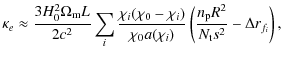
The ability of the weak-lensing cluster count (peak counting) to discriminate between the five different models chosen along the degeneracy, can be explained. If we assume that the dark matter lies at
![]() ,
which would correspond to the maximum lensing efficiency for background galaxies at z = 1, and assuming a constant dark energy model, the number density of massive clusters in the weak lensing mass maps is sensitive to both the amplitude of the mass fluctuations
,
which would correspond to the maximum lensing efficiency for background galaxies at z = 1, and assuming a constant dark energy model, the number density of massive clusters in the weak lensing mass maps is sensitive to both the amplitude of the mass fluctuations ![]() and the matter density parameter
and the matter density parameter
![]() ,
both at z=0. If instead of
,
both at z=0. If instead of ![]() ,
we consider
,
we consider
![]() ,
which represents the amplitude of the fluctuations of the projected weak lensing mass map, the
,
which represents the amplitude of the fluctuations of the projected weak lensing mass map, the
![]() is now a constant for the five models because the five corresponding weak lensing power spectrum are indistinguishable.
This leaves the
is now a constant for the five models because the five corresponding weak lensing power spectrum are indistinguishable.
This leaves the
![]() parameter which controls the structure formation (see e.g., Bahcall & Fan 1998). A low value of
parameter which controls the structure formation (see e.g., Bahcall & Fan 1998). A low value of
![]() ensures that the structures form earlier and a high
ensures that the structures form earlier and a high
![]() ensures that the structures form later. Then, for a low value of
ensures that the structures form later. Then, for a low value of
![]() ,
the abundance of massive clusters at
,
the abundance of massive clusters at
![]() become more significant (see Fig. 1 upper right) than for a high
become more significant (see Fig. 1 upper right) than for a high
![]() .
The cluster count can then be used to differentiate between cosmological models. The massive cluster abundance has already been used to probe
.
The cluster count can then be used to differentiate between cosmological models. The massive cluster abundance has already been used to probe
![]() (see e.g., Bahcall & Fan 1998).
(see e.g., Bahcall & Fan 1998).
Table 3: Discrimination efficiencies (in percent) achieved in unfiltered mass maps with the skewness estimated on the second scale of an isotropic wavelet transform.
5.2.4 Discrimination in MRLens filtered mass maps
Table 6 shows the results obtained when the MRLens filtering scheme is applied to the noisy simulated mass maps.
After MRLens filtering, the sensitivity of all transforms is greatly improved. However, the isotropic wavelet transform remains the most efficient transform certainly helped by the MRLens filtering that uses this transform.
The most effective statistic remains peak counting, which is also helped by the MRLens filtering that essentially reconstructs the clusters. However, the other statistics also achieve good results in these MRLens filtered mass maps compared to those with Gaussian filtered mass maps. This is probably because the MRLens filtering, by favoring clusters reconstruction, helps all statistics that search for non-Gaussianity.
The best result is obtained with WPC on the third scale of the isotropic wavelet transform (see Table 7). Figure 8 shows the 5 distributions that barely overlap. This statistic allows us to discriminate between different models even for adjacent models for which the discrimination is challenging.
Table 4:
Mean discrimination efficiencies (in percent) achieved on Gaussian-filtered mass maps with a false discovery rate of
![]() .
.
A comparison of these results with those obtained for noisy mass maps by the skewness in a wavelet representation (Table 3), shows that the accuracy of the constraints on ![]() and
and
![]() is improved greatly by using WPC estimated for MRLens filtered mass maps.
is improved greatly by using WPC estimated for MRLens filtered mass maps.
6 Discussion
As stated earlier, the formalism of the halo model provides a prediction of the number of clusters contained in a given field for a given cosmological model (Press and Schechter 1974; Sheth and Tormen 1999; Hamana et al. 2004). However, we have to consider that just a fraction of the clusters, present in the sky, will be detected. It follows that we have to take into account the selection effects caused by the observation quality and the data processing method. The solution that is currently used consists of modeling the selection effects by estimating the selection function. An analytic model can be developed by considering all the selection effects. An alternative consists in using a Monte Carlo approach that enables us to take into account all the selection effects that could not be considered in the analytical approach. This study will be done in a future work. When, the selection function is specified, the connection between observations and theory is straightforward. The cosmological parameters can thus be estimated from WPC.
Table 5:
Discrimination efficiencies (in percent) achieved on Gaussian-filtered mass maps with the peak counting statistic on direct space given a False Discovery Rate
![]() .
.
For a perfect differentiation between the 5 cosmological models with WPC upper limits error in the cosmological parameters can be given by considering the spacing between two adjacent models. For space observations covering 4 square degrees, the upper limit error in ![]() is 8%, in the range of
is 8%, in the range of
![]() ,
and the upper limit error in
,
and the upper limit error in
![]() is 12%, in the range of
is 12%, in the range of
![]() .
In future work, an accurate estimation of the error should be done.
.
In future work, an accurate estimation of the error should be done.
7 Conclusion
By using only two-point statistics to constrain the cosmological model, various degeneracies between cosmological parameters are possible, such as the (![]() -
-
![]() )-degeneracy. In this paper, we have considered a range of non-Gaussian statistics to attempt to place tighter constraints on cosmological parameters. For this purpose, we have run N-body simulations of 5 models selected along the (
)-degeneracy. In this paper, we have considered a range of non-Gaussian statistics to attempt to place tighter constraints on cosmological parameters. For this purpose, we have run N-body simulations of 5 models selected along the (![]() -
-
![]() )-degeneracy, and we have examined different non-Gaussian statistical tools in different representations, comparing ttheir abilities to differentiate between models. Using non-Gaussian statistics, we have searched for non-Gaussian signal for small scales caused by gravitational clustering.
)-degeneracy, and we have examined different non-Gaussian statistical tools in different representations, comparing ttheir abilities to differentiate between models. Using non-Gaussian statistics, we have searched for non-Gaussian signal for small scales caused by gravitational clustering.
Table 6:
Mean discrimination efficiencies (in percent) achieved on MRLens filtered mass maps with a false discovery rate of
![]() .
.
| |
Figure 6: Distribution of the skewness calculated from the second scale of an isotropic wavelet transform on the simulated realizations of the 5 models. It illustrates the results of the Table 3. No discrimination is possible except between the farthest models (i.e., between models 1 and 5). |
| Open with DEXTER | |
| |
Figure 7: Distribution of the peak counting estimated directly on the simulated realizations of the 5 models. It illustrates the results of the Table 5. The discrimination is possible except between adjacent models (that is to say between model 1 and model 2, model 2 and model 3, model 3 and model 4, model 4 and model 5). |
| Open with DEXTER | |
| |
Figure 8: Distribution of the wavelet peak counting estimated at the third scale of an isotropic wavelet transform on the simulated realizations of the 5 models. It illustrates the results of the Table 7. We obtain a good discrimination even for adjacent models. |
| Open with DEXTER | |
The main conclusions of our analysis are the following:
- 1.
- The isotropic wavelet transform has been found to be the best representation of the non-Gaussian structures in weak lensing data because it can differentiate between the models the most reliably.
- 2.
- We have shown that a wavelet transform denoising method such as the MRLens filtering, which reconstructs essentially the non-Gaussian structures (the clusters), helps the statistics to characterize the non-Gaussianity more reliably.
- 3.
- We have introduced a new statistic called wavelet peak counting (WPC), which consists of estimating a cluster count per scale of an isotropic wavelet transform.
- 4.
- WPC has been found to be the best statistic compared to the others that we have tested (skewness, kurtosis, bispectrum, HC, Pc), and we have shown that this statistic estimated on MRLens filtered maps provide a strong discrimination between the 5 selected models.
Another issue, discussed in Sect. 6, is selection effects. We need to determinate the selection function to estimate the cosmological parameters and accurately estimate their errors. This study will be completed in a future work.
Finally, while peak counting and WPC provide a lot of information, further statistics such as the cluster count per mass and the spatial cluster correlation will provide further constraints. Future work will be needed to fully exploit these approaches.
Appendix A: The FDR method
| |
Figure 9: Finding a threshold graphically using the FDR procedure. |
| Open with DEXTER | |
Table 7: Discrimination efficiencies (in percent) achieved on MRLens filtered mass maps with WPC on the third scale of an isotropic wavelet transform.
The false discovery rate (FDR) is a statistical approach to the multiple testing problem, introduced by Benjamini & Hochberg (1995). The FDR method offers an effective way of selecting an adaptative threshold, without any assumption. The FDR threshold is determined from the observed p-value distribution, and hence depends on the amount of signal in the data.
This technique was described by Pires et al. (2006); Hopkins et al. (2002); Miller et al. (2001); Starck et al. (2006b) for several astrophysical applications. Instead of controlling the chance of any false positives, FDR controls the expected proportion of false positives. The FDR is given by the ratio of declared active pixels (12) that are false positives, i.e.,
where
| (13) |
Where, the unknown factor
In the FDR procedure, we assume that
P1,..., Pn denote the p_values from the N tests, listed from lowest to highest and
| (14) |
where cN=1, if p_values are statistically independent.
We now declare all pixels with p_values less than or equal to Pd to be active.
Graphically, this procedure corresponds to plotting Pk versus
Appendix B: The higher criticism definition
To define HC, we first convert the individual
![]() into p-values.
Let
into p-values.
Let
![]() be the ith p-value, and p(i) denote the p-values sorted in increasing order. The higher criticism statistic is defined to be
be the ith p-value, and p(i) denote the p-values sorted in increasing order. The higher criticism statistic is defined to be
![$\displaystyle HC_n^*=\max_{\rm i}\left\vert\frac{\sqrt n [i/n-p_{(i)}]}{\sqrt{p_{(i)}(1-p_{(i)})}}\right\vert,$](/articles/aa/full_html/2009/39/aa11459-08/img109.png)
or in a modified form :
![$\displaystyle HC_n^+=\max_{i:1/n \leqslant p_{(i)} \leqslant 1-1/n}\left\vert\frac{\sqrt n [i/n-p_{(i)}]}{\sqrt{p_{(i)}(1-p_{(i)})}}\right\vert.$](/articles/aa/full_html/2009/39/aa11459-08/img110.png)
Appendix C: Description of the representations
The anisotropic bi-orthogonal wavelet transform
The most commonly used wavelet transform is the undecimated bi-orthogonal wavelet transform (OWT). Using the OWT, a 2D signal S can be decomposed as follows:
where
The undecimated isotropic wavelet transform
The undecimated isotropic wavelet transform (UIWT) decomposes an
![]() image
image ![]() into :
into :
where CJ is a coarse or smooth version of the original image
The ridgelet transform
Classical multiresolution methods address only a portion of the entire range of interesting phenomena which is roughly isotropic one on all scales and at all locations. The ridgelet transform was proposed as an alternative to the wavelet representation of image data.
Given a function
f(x1,x2), the ridgelet transform is the superposition
of elements of the form
![]() ,
,
![]() is the wavelet, a > 0 the scale parameter, b the location parameter, and
is the wavelet, a > 0 the scale parameter, b the location parameter, and ![]() the orientation parameter. The ridgelet is constant along lines
the orientation parameter. The ridgelet is constant along lines
![]() ,
and, transverse to these ridges, it is a wavelet.
,
and, transverse to these ridges, it is a wavelet.
The curvelet transform
Ridgelets essentially focus on straight lines rather than curves. However they can be adapted to representing objects with curved edges using an appropriate multiscale localization. If one uses a sufficiently fine scale to capture curved edges, such edges are almost straight. As a consequence, the curvelet transform has been introduced, in which ridgelets are used in a localized manner.
The idea of the curvelet transform (Candès and Donoho 1999; Starck et al. 2003) is to first decompose the image into a set of wavelet planes, then decompose each plane into several blocks (the block size can change on each scale level) before finally analyzing each block with a ridgelet transform. The finer the scale, the more sensitive to the curvature the analysis is. As a consequence, curved singularities can be well represented with very few coefficients.
Appendix D: The MRLens filtering
The MRLens filtering (Starck et al. 2006b) is a non-linear filtering based on Bayesian theory that searches for a solution maximizing the a posteriori probability. Choosing the prior is one of the most critical aspects of Bayesian analysis. The MRLens filtering uses a multiscale entropy prior.
Assuming Gaussian noise, the MRlens filtering solves the minimization
 |
(19) |
where
In Starck et al. (2006b), it was shown that the MRLens filtering outperforms the existing methods. The MRLens
![]() filtering has already been used in several applications to weak lensing data, and was in partocular selected to filter the dark-matter mass map obtained by the Hubble Space Telescope in the COSMOS field.
filtering has already been used in several applications to weak lensing data, and was in partocular selected to filter the dark-matter mass map obtained by the Hubble Space Telescope in the COSMOS field.
References
Footnotes
- ... MRLens
![[*]](/icons/foot_motif.png)
- The MRLens software is available at the following address: http://www-irfu.cea.fr/Ast/878.html
- ... MRLens
- The complete MRLens software package to perform weak lensing filtering can be downloaded from http://www-irfu.cea.fr/Ast/878.html
All Tables
Table 1:
Parameters of the five cosmological models that have been chosen along the (
![]() )-degeneracy.
)-degeneracy.
Table 2:
Mean discrimination efficiencies (in percent) achieved on noisy mass maps with a false discovery rate of
![]() .
.
Table 3: Discrimination efficiencies (in percent) achieved in unfiltered mass maps with the skewness estimated on the second scale of an isotropic wavelet transform.
Table 4:
Mean discrimination efficiencies (in percent) achieved on Gaussian-filtered mass maps with a false discovery rate of
![]() .
.
Table 5:
Discrimination efficiencies (in percent) achieved on Gaussian-filtered mass maps with the peak counting statistic on direct space given a False Discovery Rate
![]() .
.
Table 6:
Mean discrimination efficiencies (in percent) achieved on MRLens filtered mass maps with a false discovery rate of
![]() .
.
Table 7: Discrimination efficiencies (in percent) achieved on MRLens filtered mass maps with WPC on the third scale of an isotropic wavelet transform.
All Figures
| |
Figure 1:
Upper left, the 5 cosmological models along the (
|
| Open with DEXTER | |
| In the text | |
| |
Figure 2:
The following two distributions correspond to the histogram of the values of a given statistic estimated on the 100 realizations of model 1 (m1) and on the 100 realizations of model 2 (m2). The discrimination achieved with this statistic between m1 and m2 is rather good: the two distributions barely overlap. To characterize the discrimination more quantitatively, the FDR method has been used to estimate the thresholds
|
| Open with DEXTER | |
| In the text | |
| |
Figure 3:
Left: noiseless simulated mass map and right: simulated noisy mass map that we should obtain in space observations. The field is 1.975
|
| Open with DEXTER | |
| In the text | |
| |
Figure 4:
Left, noiseless simulated mass map, and right, filtered mass map by convolution with a Gaussian kernel. The field is 1.975
|
| Open with DEXTER | |
| In the text | |
| |
Figure 5:
Left, noiseless simulated mass map, and right, filtered mass map by the FDR multiscale entropy filtering. The field is 1.975
|
| Open with DEXTER | |
| In the text | |
| |
Figure 6: Distribution of the skewness calculated from the second scale of an isotropic wavelet transform on the simulated realizations of the 5 models. It illustrates the results of the Table 3. No discrimination is possible except between the farthest models (i.e., between models 1 and 5). |
| Open with DEXTER | |
| In the text | |
| |
Figure 7: Distribution of the peak counting estimated directly on the simulated realizations of the 5 models. It illustrates the results of the Table 5. The discrimination is possible except between adjacent models (that is to say between model 1 and model 2, model 2 and model 3, model 3 and model 4, model 4 and model 5). |
| Open with DEXTER | |
| In the text | |
| |
Figure 8: Distribution of the wavelet peak counting estimated at the third scale of an isotropic wavelet transform on the simulated realizations of the 5 models. It illustrates the results of the Table 7. We obtain a good discrimination even for adjacent models. |
| Open with DEXTER | |
| In the text | |
| |
Figure 9: Finding a threshold graphically using the FDR procedure. |
| Open with DEXTER | |
| In the text | |
Copyright ESO 2009
Current usage metrics show cumulative count of Article Views (full-text article views including HTML views, PDF and ePub downloads, according to the available data) and Abstracts Views on Vision4Press platform.
Data correspond to usage on the plateform after 2015. The current usage metrics is available 48-96 hours after online publication and is updated daily on week days.
Initial download of the metrics may take a while.