| Issue |
A&A
Volume 505, Number 2, October II 2009
|
|
|---|---|---|
| Page(s) | 825 - 843 | |
| Section | Planets and planetary systems | |
| DOI | https://doi.org/10.1051/0004-6361/200911765 | |
| Published online | 28 July 2009 | |
A&A 505, 825-843 (2009)
Interferometric imaging of carbon monoxide in comet C/1995 O1 (Hale-Bopp): evidence of a strong rotating jet
D. Bockelée-Morvan1 - F. Henry1 - N. Biver1 - J. Boissier2 - P. Colom1 - J. Crovisier1
- D. Despois3 - R. Moreno1 - J. Wink2,![]()
1 - Observatoire de Paris, 92195 Meudon, France
2 - IRAM, 300 rue de la Piscine, Domaine universitaire, 38406 Saint Martin d'Hères, France
3 -
Observatoire de Bordeaux, BP 89, 33270 Floirac, France
Received 2 February 2009 / Accepted 22 June 2009
Abstract
Context. Observations of the CO J(1-0) 115 GHz and J(2-1) 230 GHz lines in comet C/1995 O1 (Hale-Bopp) were performed with the IRAM Plateau de Bure interferometer on 11 March, 1997. The observations were conducted in both single-dish (ON-OFF) and interferometric modes with 0.13 km s-1 spectral resolution. Images of CO emission of between 1.7 and 3
![]() angular resolution were obtained.
angular resolution were obtained.
Aims. The ON-OFF and interferometric spectra show a velocity shift with sinusoidal time variations related to the Hale-Bopp nucleus rotation of 11.35 h. The peak position of the CO images moves perpendicularly to the spin axis direction in the plane of the sky. This suggests that a CO jet is present, is active night and day with about the same extent, and is spiralling according to the nucleus rotation. The high quality of the data allows us to constrain the characteristics of this CO jet.
Methods. We developed a 3D model to interpret the temporal evolution of CO spectra and maps. The CO coma is represented as the combination of an isotropic distribution and a spiralling gas jet, both of nucleus origin.
Results. The analysis of the spectra and visibilities obtained from the interferometric data shows that the CO jet contains ![]() 40% of the total CO production and is located close to the nucleus equator at a latitude
40% of the total CO production and is located close to the nucleus equator at a latitude ![]() 20
20![]() north. Our inability to reproduce all observational characteristics shows that the true structure of the CO coma is more complex than assumed, especially within the first thousand kilometres from the nucleus. The presence of another moving CO structure, faint but compact and possibly created by an outburst, is identified.
north. Our inability to reproduce all observational characteristics shows that the true structure of the CO coma is more complex than assumed, especially within the first thousand kilometres from the nucleus. The presence of another moving CO structure, faint but compact and possibly created by an outburst, is identified.
Key words: comets: individual: C/1995 O1 - radio lines: solar system - techniques: interferometric
1 Introduction
Millimetre spectroscopy has provided many insights into
the composition and physical properties of cometary atmospheres.
Many cometary parent molecules originating in the nucleus were identified
with this technique. The high spectral resolution capabilities, and
the possibility to observe several rotational lines belonging to
the same molecule, has allowed us to retrieve unique information about the
velocity and temperature of the expanding coma, and the anisotropy of gas
production at the nucleus surface. Because of the low, diffraction-limited
spatial resolution provided by radio dishes at millimetre wavelengths,
at best typically 10
![]() ,
studies concerning the spatial distribution of
parent molecules in the coma have been rare.
,
studies concerning the spatial distribution of
parent molecules in the coma have been rare.
The exceptional brightness of comet C/1995 O1 (Hale-Bopp) close to its perihelion on 1 April, 1997, motivated a wealth of innovative cometary observations. Among them, interferometric imaging of rotational transitions of parent
molecules was successfully attempted. The Berkeley-Illinois-Maryland
Association (BIMA) array mapped comet
Hale-Bopp in HCN J(1-0) and CS J(2-1) with 9
![]() angular
resolution. Spatial asymmetries, implying the presence of gas
jets, were detected (Wright et al. 1998; Woodney et al. 2002; Veal et al. 2000).
Constraints on the photodissociative
scalelengths of HCN and CS were obtained from the radial extent of
their radio emissions (Snyder et al. 2001). Using the Owens Valley
Radio Observatory (OVRO) millimetre array, Blake et al. (1999)
obtained maps of HCN, DCN, HNC, and HDO at spatial resolutions of 2-4
angular
resolution. Spatial asymmetries, implying the presence of gas
jets, were detected (Wright et al. 1998; Woodney et al. 2002; Veal et al. 2000).
Constraints on the photodissociative
scalelengths of HCN and CS were obtained from the radial extent of
their radio emissions (Snyder et al. 2001). Using the Owens Valley
Radio Observatory (OVRO) millimetre array, Blake et al. (1999)
obtained maps of HCN, DCN, HNC, and HDO at spatial resolutions of 2-4
![]() over
2-3 h integration time.
The presence of arc-like structures offset from the nucleus is reported
for all species apart from HCN, and interpreted in terms of jets of icy particles
releasing unalterated gas in contrast to that outgassed from the nucleus.
over
2-3 h integration time.
The presence of arc-like structures offset from the nucleus is reported
for all species apart from HCN, and interpreted in terms of jets of icy particles
releasing unalterated gas in contrast to that outgassed from the nucleus.
Interferometric observations of rotational lines in comet
Hale-Bopp were also made with the Plateau de Bure interferometer
(PdBI) of the Institut de Radio Astronomie Millimétrique (IRAM)
at a resolution of 1-3
![]() .
A short and preliminary account of
these observations was given in Wink et al. (1999), Despois (1999), and
Henry et al. (2002). Millimetre lines of CO, HCN, CS, HNC, CH3OH,
H2S, SO, and H2CO were mapped (Wink et al. 1999; Boissier et al. 2007). At the same
time, continuum maps of the dust and nucleus thermal emissions
were obtained (Altenhoff et al. 1999). The PdBI was also used in
single-dish mode to detect new cometary molecules
(Crovisier et al. 2004a,b; Bockelée-Morvan et al. 2000).
.
A short and preliminary account of
these observations was given in Wink et al. (1999), Despois (1999), and
Henry et al. (2002). Millimetre lines of CO, HCN, CS, HNC, CH3OH,
H2S, SO, and H2CO were mapped (Wink et al. 1999; Boissier et al. 2007). At the same
time, continuum maps of the dust and nucleus thermal emissions
were obtained (Altenhoff et al. 1999). The PdBI was also used in
single-dish mode to detect new cometary molecules
(Crovisier et al. 2004a,b; Bockelée-Morvan et al. 2000).
We present observations of the CO J(1-0) (115 GHz) and
J(2-1) (230 GHz) lines, performed
on 11 March 1997, at the Plateau de Bure interferometer. Among the ![]() 20
molecules identified in comet Hale-Bopp, and in general in
cometary atmospheres, carbon monoxide CO is of particular interest for the following reasons:
20
molecules identified in comet Hale-Bopp, and in general in
cometary atmospheres, carbon monoxide CO is of particular interest for the following reasons:
- 1.
- This species is the main agent of distant cometary activity, as first demonstrated for comet 29P/Schwassmann-Wachmann 1 (Crovisier et al. 1995; Senay & Jewitt 1994). This was later confirmed
for comet Hale-Bopp from its long-term monitoring, which showed the change
from a CO-dominated to an H2O-dominated activity at heliocentric distances
 -4 AU (Biver et al. 1999a,1997).
- 2.
- In comets within 3 AU from the Sun, CO is, most often, the second major
gaseous component of the coma after water. CO production rates
relative to water are highly variable from comet to comet, ranging from less than 1% to
 20% (Irvine et al. 2000; Bockelée-Morvan et al. 2004, for a review).
The value obtained in comet Hale-Bopp near perihelion is among the highest ever observed in comets: 20%
(e.g., DiSanti et al. 2001; Bockelée-Morvan et al. 2000).
20% (Irvine et al. 2000; Bockelée-Morvan et al. 2004, for a review).
The value obtained in comet Hale-Bopp near perihelion is among the highest ever observed in comets: 20%
(e.g., DiSanti et al. 2001; Bockelée-Morvan et al. 2000).
- 3.
- There continues to be much debate about CO production mechanisms. Because CO has a low sublimation temperature, the nucleus surface certainly contains a small amount of CO ice. Therefore, CO should outgass at some depth inside the nucleus, possibly from pure CO ice sublimation and/or from amorphous water ice when crystallizing and releasing trapped molecules (e.g., Enzian et al. 1998; Capria et al. 2002,2000), if indeed pre-cometary ices condensed in amorphous form, something that is somewhat debated (Mousis et al. 2000). Another mechanism proposed to explain the CO production of comet Hale-Bopp near perihelion is the release of CO trapped in crystalline water ice during water ice sublimation (Capria et al. 2002,2000). Comparing the CO jet morphology, as the nucleus rotates, to those of less volatile species or dust might provide clues to the origin of CO.
- 4.
- There are several pieces of
observational evidence that a significant part of the CO observed
in cometary atmospheres could be produced by a distributed source.
From in situ measurements of the local CO density in 1P/Halley
with Giotto, Eberhardt et al. (1987) concluded that only about 1/3 of the CO
originated in the nucleus. The spatial distribution of CO
molecules deduced from infrared long-slit observations of comet
Hale-Bopp led DiSanti et al. (2001,1999) to suggest that one-half of
the CO was released by a distributed source when comet Hale-Bopp
was within 1.5 AU from the Sun. The spatial resolution of the CO
maps obtained at PdBI, which corresponded approximately 1000 km to 1700 km radius
on the comet depending on the line observed, is below the
estimated radial extension of the CO distributed source of
 km (DiSanti et al. 2001; Brooke et al. 2003). Therefore, an
important aspect of the study of the CO PdBI interferometric data
is that independent information about the existence of a CO
distributed source in Hale-Bopp coma can possibly be obtained. The
study of the radial distribution of the CO molecules is presented
in a separate paper (Bockelée-Morvan & Boissier 2009). The brightness distribution of
both 115 GHz and 230 GHz lines can be fully explained by pure
nuclear CO production, provided that opacity effects and
temperature variations in the coma are taken into account
(Bockelée-Morvan & Boissier 2009; Bockelée-Morvan et al. 2005).
km (DiSanti et al. 2001; Brooke et al. 2003). Therefore, an
important aspect of the study of the CO PdBI interferometric data
is that independent information about the existence of a CO
distributed source in Hale-Bopp coma can possibly be obtained. The
study of the radial distribution of the CO molecules is presented
in a separate paper (Bockelée-Morvan & Boissier 2009). The brightness distribution of
both 115 GHz and 230 GHz lines can be fully explained by pure
nuclear CO production, provided that opacity effects and
temperature variations in the coma are taken into account
(Bockelée-Morvan & Boissier 2009; Bockelée-Morvan et al. 2005).
2 Observations
2.1 Description
Comet C/1995 O1 (Hale-Bopp) was observed from 6 March to 22 March, 1997 with the Plateau de Bure interferometer of IRAM, located in the French Alps. The observations of the J(2-1) (230.538 GHz) and J(1-0) (115.271 GHz) CO rotational transitions were carried out on 11 March, from 4h to 15h UT. On this day, comet Hale-Bopp was at the geocentric distance
![]() AU and heliocentric distance
AU and heliocentric distance
![]() AU. The weather conditions were good to excellent and the atmospheric seeing was
AU. The weather conditions were good to excellent and the atmospheric seeing was ![]() 0.4
0.4
![]() for both 1.3 and 3 mm receivers.
for both 1.3 and 3 mm receivers.
The comet was tracked using orbital elements provided by Yeomans (JPL, solution 55). The ephemeris was computed by Rocher
(IMCCE, Observatoire de Paris) with a program that takes into
account planetary perturbations. The first interferometric maps
obtained on 9 March (HCN J(1-0) line) inferred that both
continuum and molecular peak intensities were offset by about
5-6
![]() North in declination (Dec) from the nucleus position
provided by the ephemeris. Observations on March 11 were performed with
the ephemeris corrected by 6
North in declination (Dec) from the nucleus position
provided by the ephemeris. Observations on March 11 were performed with
the ephemeris corrected by 6
![]() North in Dec.
North in Dec.
The PdBI was used in the compact configuration C1 (see Fig. 1) with five 15-m antennas providing 10 baselines (the spacing between two antennas) ranging from ![]() 20 to
20 to ![]() 150 m. In 1997, the PdBI comprised a flexible spectral correlator made of six independent units, providing correlated spectra with 64 to 256 channels spaced by between 0.039 MHz and 2.5 MHz. We used 256 channels of 78 kHz separation for the observations of the 230 GHz line, and 256 channels of 39 kHz separation for those of
the 115 GHz line. The four other units were used for the continuum
observations presented in Altenhoff et al. (1999). The effective spectral resolution is a factor of 1.3 broader than the channel spacing, and corresponds to
150 m. In 1997, the PdBI comprised a flexible spectral correlator made of six independent units, providing correlated spectra with 64 to 256 channels spaced by between 0.039 MHz and 2.5 MHz. We used 256 channels of 78 kHz separation for the observations of the 230 GHz line, and 256 channels of 39 kHz separation for those of
the 115 GHz line. The four other units were used for the continuum
observations presented in Altenhoff et al. (1999). The effective spectral resolution is a factor of 1.3 broader than the channel spacing, and corresponds to ![]() 0.13 km s-1 for both lines.
0.13 km s-1 for both lines.
![\begin{figure}
\par\resizebox{9cm}{!}{\includegraphics[angle=270]{117651.ps}}
\end{figure}](/articles/aa/full_html/2009/38/aa11765-09/img33.png) |
Figure 1: The Plateau de Bure Interferometer in C1 configuration |
| Open with DEXTER | |
The observing cycle was : pointing, focusing, 4 min of
cross-correlation on the calibrators (2200+420 BL Lac,
MWC349 and 3C373), 2 min of autocorrelation, and 51 one min scans
of cross-correlation on the comet interlaced with scans on the
phase calibrator (2200+420 BL Lac) observed every 20 min. The cycle
was completed by another
2 min of autocorrelation on Hale-Bopp. For the autocorrelation
observations (in this mode, the five antennas behave as five independent
single-dish telescopes), we used position-switching (ON-OFF) with a 5![]() offset to remove the sky background. The spectra of the five
antennas were then coadded. Hereafter, these autocorrelation
observations are referred to as ON-OFF observations.
offset to remove the sky background. The spectra of the five
antennas were then coadded. Hereafter, these autocorrelation
observations are referred to as ON-OFF observations.
The amplitude and phase calibrator was 2200+420. MWC349 was used to determine the flux density of 2200+420. Bandpass calibration was made on 3C273. Because of the lower accuracy of the phase calibration after 12.5 h UT, only interferometric data
acquired before 12.5 h UT were considered. Calibration was done with the IRAM CLIC software, and the data hence derived were stored in uv-tables. Reduction and cleaning of the maps were performed with the MAPPING/GILDAS software![]() .
.
Concerning ON-OFF spectra, antenna temperatures
![]() were converted into main beam brightness temperatures
were converted into main beam brightness temperatures
![]() by means of
by means of
![]() with
beam efficiencies
with
beam efficiencies
![]() of 0.83 and 0.58, at 115 GHz and 230 GHz, respectively, and forward efficiencies
of 0.83 and 0.58, at 115 GHz and 230 GHz, respectively, and forward efficiencies
![]() of 0.93 and
0.89, at 115 GHz and 230 GHz, respectively. Flux density per beam (S in Jy) is then related to antenna
temperature by means of
of 0.93 and
0.89, at 115 GHz and 230 GHz, respectively. Flux density per beam (S in Jy) is then related to antenna
temperature by means of
![]() ,
where
,
where
![]() is the main beam solid angle. For both ON-OFF and interferometric data, the uncertainties in flux calibration are at most 10% and 15% for the J(1-0) and J(2-1) lines, respectively. The rms in phase noise ranges from 10 to 27
is the main beam solid angle. For both ON-OFF and interferometric data, the uncertainties in flux calibration are at most 10% and 15% for the J(1-0) and J(2-1) lines, respectively. The rms in phase noise ranges from 10 to 27![]() at 230 GHz and from 4.6 to 20
at 230 GHz and from 4.6 to 20![]() at 115 GHz,
depending on the baseline.
at 115 GHz,
depending on the baseline.
For each spectral channel, the cross-correlated spectra produce
interferometric maps with spatial resolutions determined by the
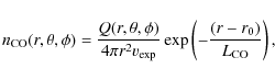
uv-coverage (Fig. 2). When all cross-correlation
data are considered, the full width at half maximum (FWHM) of the
synthesized beam is 2.00
![]()
![]() 1.38
1.38
![]() with
major axis at position angle pa=99.56
with
major axis at position angle pa=99.56![]() at 230 GHz, and
3.58
at 230 GHz, and
3.58
![]()
![]() 2.57
2.57
![]() with pa=86.00
with pa=86.00![]() at 115
GHz. The FWHM of the primary beam of the antennas is 20.9
at 115
GHz. The FWHM of the primary beam of the antennas is 20.9
![]() at 230 GHz, and 41.8
at 230 GHz, and 41.8
![]() at 115 GHz.
at 115 GHz.
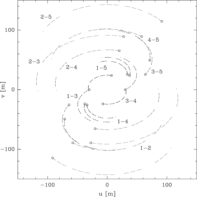 |
Figure 2: uv-coverage at the PdBI on 11 March, 1997 with the C1 configuration. For each arc of ellipse, the white circle represents the uv-point at the beginning of the observations. The time evolution of the uv-points loci is counterclockwise. |
| Open with DEXTER | |
![\begin{figure}
\par {\includegraphics[bb = 110 248 481 543,angle=0,width=18cm,
clip=true]{117653.ps} }
\end{figure}](/articles/aa/full_html/2009/38/aa11765-09/img44.png) |
Figure 3: CO J(2-1) spectra obtained in ON-OFF and interferometric modes as a function of time, given in UT hours on 11 March, 1997. The velocity scale is with respect to the comet rest velocity. Spectra have been shifted vertically according to observation time, but are scaled identically. a) ON-OFF spectra: the integration time is 2 min (on+off); b-d) interferometric spectra (visibility amplitude as a function of spectral channel): averages of 25 to 27 scans of 1 min. Only data for the 3 shortest baselines are shown. |
| Open with DEXTER | |
2.2 ON-OFF spectra
ON-OFF spectra of the CO J(2-1) line are shown in Fig. 3a. The integration time is 2 min (on+off) for each spectrum. They show a feature moving from positive to negative velocities, and back to positive velocities again, with respect to the nucleus velocity frame. In other words, a jet-like CO gas feature, with a velocity vector that has rotated with respect to Earth during the course of the observations, is observed. This CO gas feature contributes to as much as 28% of the total line area.
The synodic rotation period of comet Hale-Bopp in February-April 1997 was
deduced from studies of the dust shells (Sarmecanic et al. 1997; Ortiz & Rodríguez 1999; Farnham et al. 1999). The most accurate value
![]() h measured by Farnham et al. (1999)
agrees with a slightly longer sidereal rotation period of P = 11.34
h measured by Farnham et al. (1999)
agrees with a slightly longer sidereal rotation period of P = 11.34 ![]() 0.02 h (Jorda et al. 1999; Licandro et al. 1998). Figure 4 plots the evolution in the
line velocity shift (the spectrum first order momentum) with time. The points
follow a sinusoidal curve of period corresponding to the comet's nucleus
rotation (taken to equal 11.35 h throughout this paper).
The sinusoid determined from a least squares fit of fixed period P = 11.35 h has a mean level of
0.02 h (Jorda et al. 1999; Licandro et al. 1998). Figure 4 plots the evolution in the
line velocity shift (the spectrum first order momentum) with time. The points
follow a sinusoidal curve of period corresponding to the comet's nucleus
rotation (taken to equal 11.35 h throughout this paper).
The sinusoid determined from a least squares fit of fixed period P = 11.35 h has a mean level of
![]() km s-1 and its amplitude is
km s-1 and its amplitude is
![]() km s-1 (Fig. 4). The line area does not show significant variation with time, and has a mean value of
km s-1 (Fig. 4). The line area does not show significant variation with time, and has a mean value of
![]() K km s-1 in main beam brightness temperature scale
K km s-1 in main beam brightness temperature scale
![]() (i.e., 82.8 Jy km s-1 in flux density scale).
Fluctuations of
(i.e., 82.8 Jy km s-1 in flux density scale).
Fluctuations of ![]() 10% at most are observed (with a standard deviation of 5%), which are not correlated with the velocity shift variations. The velocity shift curve obtained for the J(1-0) line is much more noisy (errorbars
10% at most are observed (with a standard deviation of 5%), which are not correlated with the velocity shift variations. The velocity shift curve obtained for the J(1-0) line is much more noisy (errorbars ![]() 0.2 km s-1 in
individual spectra), but is similar to the J(2-1) velocity shift curve:
a least squares sinusoid fit with P fixed to 11.35 h leads to
0.2 km s-1 in
individual spectra), but is similar to the J(2-1) velocity shift curve:
a least squares sinusoid fit with P fixed to 11.35 h leads to
![]() km s-1,
km s-1,
![]() km s-1 (Henry 2003).
Adding all spectra, the mean velocity shift of the J(1-0) line is
-0.09
km s-1 (Henry 2003).
Adding all spectra, the mean velocity shift of the J(1-0) line is
-0.09 ![]() 0.05 km s-1, in agreement
with that of the J(2-1) line (-0.083
0.05 km s-1, in agreement
with that of the J(2-1) line (-0.083 ![]() 0.007 km s-1). The line area of the J(1-0) line is 0.552
0.007 km s-1). The line area of the J(1-0) line is 0.552 ![]() 0.022 K km s-1 in the
0.022 K km s-1 in the
![]() scale (i.e., 10.8 Jy km s-1).
scale (i.e., 10.8 Jy km s-1).
![\begin{figure}
\par\resizebox{9cm}{!}{\includegraphics[angle=270]{117654.ps}}
\end{figure}](/articles/aa/full_html/2009/38/aa11765-09/img51.png) |
Figure 4:
Time evolution of the velocity shift of CO J(2-1) ON-OFF spectra shown in Fig. 3a.
The plotted curve is the least squares sinusoid fit to the data.
It has a fixed period of 11.35 h, an amplitude of
|
| Open with DEXTER | |
From the spin axis orientation and the equatorial coordinates of the comet,
it is possible to derive the angle
![]() (aspect angle) between the spin axis
and the line of sight, and the North pole position
angle
(aspect angle) between the spin axis
and the line of sight, and the North pole position
angle
![]() ,
defined from North to East.
The different spin orientations published in the literature are listed in
Table 1.
,
defined from North to East.
The different spin orientations published in the literature are listed in
Table 1.
Table 1: Spin axis orientation.
Adopting the spin orientation derived by Jorda et al. (1999) and Schleicher et al. (2004),
the comet spin axis was then only 20![]() from the plane of the sky.
In this geometrical configuration, a polar CO jet would lead to an almost
constant velocity shift. A jet close to the equator can explain a
velocity shift following a sinusoid centred around
from the plane of the sky.
In this geometrical configuration, a polar CO jet would lead to an almost
constant velocity shift. A jet close to the equator can explain a
velocity shift following a sinusoid centred around ![]()
![]() 0 km s-1. Both this sinusoidal curve and the constant CO line area indicate that the amount of CO gas released in this jet did not vary
during nucleus rotation. Given the Sun direction (phase angle of 46
0 km s-1. Both this sinusoidal curve and the constant CO line area indicate that the amount of CO gas released in this jet did not vary
during nucleus rotation. Given the Sun direction (phase angle of 46![]() ,
pa = 160
,
pa = 160![]() ), this near-equatorial CO jet was active day and night with about the same extent.
), this near-equatorial CO jet was active day and night with about the same extent.
From the line areas of the J(1-0) and J(2-1) ON-OFF
profiles, we derive a CO production rate
![]() s-1. Here, we assumed a Haser parent
molecule distribution for CO, and run our excitation model (Sect. 3) with a kinetic temperature T of 120 K which
agrees with temperature determinations pertaining to the
10 000-20 000 km (radius) coma region sampled by the primary
beam of PdBI (DiSanti et al. 2001; Biver et al. 1999a). Using an extended
production for CO consistent with the IR observations does not
significantly affect the inferred
s-1. Here, we assumed a Haser parent
molecule distribution for CO, and run our excitation model (Sect. 3) with a kinetic temperature T of 120 K which
agrees with temperature determinations pertaining to the
10 000-20 000 km (radius) coma region sampled by the primary
beam of PdBI (DiSanti et al. 2001; Biver et al. 1999a). Using an extended
production for CO consistent with the IR observations does not
significantly affect the inferred
![]() .
DiSanti et al. (2001)
inferred a total CO production rate (nuclear+distributed) fully
consistent with our value. In the following sections, we assume
T = 120 K and a total
.
DiSanti et al. (2001)
inferred a total CO production rate (nuclear+distributed) fully
consistent with our value. In the following sections, we assume
T = 120 K and a total
![]() of
of
![]() s-1.
s-1.
2.3 Interferometric data
![\begin{figure}
\par {\includegraphics[width=8.8cm,angle=270]{117655a.ps} }
\vspace{+0.8cm}
{\includegraphics[width=8.8cm,angle=270]{117655b.ps} }
\end{figure}](/articles/aa/full_html/2009/38/aa11765-09/img58.png) |
Figure 5:
CO J(1-0) ( top) and J(2-1) ( bottom) line integrated maps observed on 11 March, 1997 (all data). Twenty-five spectral channels have been averaged. The synthesized beam is in the lower left. The dashed square on the J(1-0) map corresponds to the size of the J(2-1) map. For the CO J(1-0) line, contours are 0.037 Jy/beam,
and the rms is 0.018 Jy/beam. For the J(2-1) line, contours are 0.186 Jy/beam and the rms is 0.066 Jy/beam. Iso-contours are successive multiples of 10% of the maximum intensity, at 10 to 100% of the maximum intensity. The solar direction is indicated. The original images have been shifted so that the maximum brightness peaks at the centre of the maps. In units of line area, the intensities at maximum brightness are
|
| Open with DEXTER | |
We present in Fig. 5 the line integrated maps of CO J(2-1) and J(1-0). Eight hours of observations were averaged (from 4.5 h UT to 12.5 h UT) and 25 velocity channels (12 on both sides of the central channel corresponding to the nucleus velocity) were coadded. An asymmetrical shape, which is not aligned with the elliptical clean beam (the synthesized interferometer beam), is observed and related to the anisotropy of the gas emission.
In the line integrated interferometric map of CO J(2-1) (Fig. 5), the position of the peak brightness (![]() )
is at RA = 22
)
is at RA = 22![]() 30
30![]() 38.02
38.02![]() and Dec = 40
and Dec = 40![]() 46
46![]() 3.1
3.1
![]() (with an astrometric precision of
0.07
(with an astrometric precision of
0.07
![]() )
in apparent geocentric coordinates given for 7.00 h UT.
The peak position of the CO J(1-0) brightness (RA = 22
)
in apparent geocentric coordinates given for 7.00 h UT.
The peak position of the CO J(1-0) brightness (RA = 22![]() 29
29![]() 38.46
38.46![]() and Dec = 40
and Dec = 40![]() 41
41![]() 10.1
10.1
![]() at 4.00 h
UT) is consistent with that of J(2-1), taking into account the
comet motion from 4 to 7 h UT (see Boissier et al. 2007). The peak
position of the continuum emission at 230 GHz observed
simultaneously also almost coincides (0.2
at 4.00 h
UT) is consistent with that of J(2-1), taking into account the
comet motion from 4 to 7 h UT (see Boissier et al. 2007). The peak
position of the continuum emission at 230 GHz observed
simultaneously also almost coincides (0.2
![]() offset) with the
CO J(2-1) peak (Boissier et al. 2007; Altenhoff et al. 1999).
Using orbital elements based on optical astrometric positions
from April 1996 to August 2005 (JPL solution 220),
the offset between the CO peak and the ephemeris is
+2.9
offset) with the
CO J(2-1) peak (Boissier et al. 2007; Altenhoff et al. 1999).
Using orbital elements based on optical astrometric positions
from April 1996 to August 2005 (JPL solution 220),
the offset between the CO peak and the ephemeris is
+2.9
![]() in Dec and +0.4
in Dec and +0.4
![]() in RA. Therefore, positions of the
CO and radio continuum brightness peaks differ by typically
+3
in RA. Therefore, positions of the
CO and radio continuum brightness peaks differ by typically
+3
![]() in Dec from optical astrometric positions. A bright
dusty jet was identified southward in the optical images of comet
Hale-Bopp near perihelion (e.g., Jorda et al. 1999). As shown by
Boissier et al. (2007), the optical astrometric positions were more
affected by dusty jets than the radio positions. Boissier et al. (2007) showed
that the astrometric positions provided by the IRAM continuum radio maps
inferred an orbit that does not require the existence of
non-gravitational forces acting on the Hale-Bopp nucleus, in
contrast to those derived from only optical positions, thereby
solving a contentious issue. In conclusion, there
is no substantial offset between the nucleus position and the mean
photometric centre of CO emission.
in Dec from optical astrometric positions. A bright
dusty jet was identified southward in the optical images of comet
Hale-Bopp near perihelion (e.g., Jorda et al. 1999). As shown by
Boissier et al. (2007), the optical astrometric positions were more
affected by dusty jets than the radio positions. Boissier et al. (2007) showed
that the astrometric positions provided by the IRAM continuum radio maps
inferred an orbit that does not require the existence of
non-gravitational forces acting on the Hale-Bopp nucleus, in
contrast to those derived from only optical positions, thereby
solving a contentious issue. In conclusion, there
is no substantial offset between the nucleus position and the mean
photometric centre of CO emission.
![\begin{figure}
\par {\includegraphics[angle=270,width=17cm]{117656a.ps} }
\vspace{+0.8cm}
{\includegraphics[angle=270,width=17cm]{117656b.ps} }
\end{figure}](/articles/aa/full_html/2009/38/aa11765-09/img62.png) |
Figure 6:
CO maps as a function of spectral channel on 11 March, 1997 (all data averaged). RA and Dec positions are with respect to the mean photometric centre |
| Open with DEXTER | |
![\begin{figure}
\par\includegraphics[angle=270,width=17cm]{117657.ps}
\end{figure}](/articles/aa/full_html/2009/38/aa11765-09/img63.png) |
Figure 7:
Individual maps of CO J(2-1) for data subsets of 1 h. Isocontours are successive multiples of 10% of the maximum
intensity, at 10 to 100% of the maximum intensity. For each map labelled (i) on the top left corners, a cross identifies the mean photometric centre |
| Open with DEXTER | |
The J(1-0) and J(2-1) spectral channel maps (Fig. 6) were obtained with the same procedure. The peak brightness in the blue channels is stronger than that in the red ones. This indicates that there is more emission toward the Earth, which is consistent with the ON-OFF spectra. The interferometric observations indeed covered only 2/3 of the nucleus rotation period, when the jet was, most of the time, facing the Earth (Fig. 4). The spectral maps show that the CO coma structure is complex. The interpretation of the brightness distribution on these maps is not straightforward, since the signal is here averaged over the entire period of observation and the CO coma is rotating. The most central channels are sensitive to molecules expanding along directions close to the plane of the sky. They exhibit coma structures towards north-west and south-east quadrants (roughly along a direction perpendicular to the projected rotation axis; see the 230 GHz maps in Fig. 6). These structures may trace the jet at the time that it was near the plane of the sky. Channels at high negative velocities (-0.6 to -0.9 km s-1) show a much brighter and strongly peaked intensity distribution because the jet is here facing the Earth.
To investigate whether there is temporal evidence for the
rotating jet in the images of the CO emission, we combined
five separate subdivisions of about 1 h each. Resulting maps are
presented in Fig. 7. Because of Earth's rotation, the
beam shape rotates with time from map to map and changes dimension
(see next paragraph). This prevents a detailed study of the
rotating jets directly from the maps and, as explained later,
another approach will be used. However, an interesting feature is
observed. From the observations averaged over the entire day, we
derived the mean photometric centre of CO emission, ![]() .
For each map i, we can also derive the photometric centre,
.
For each map i, we can also derive the photometric centre,
![]() ,
and the vector
,
and the vector
![]() ,
as shown in Fig. 7. The time evolution of
,
as shown in Fig. 7. The time evolution of
![]() is presented in Fig. 8. We observe that it moves counterclockwise (disregarding
is presented in Fig. 8. We observe that it moves counterclockwise (disregarding ![]() )
along an ellipse, whose
long axis is perpendicular to the spin axis direction. This
displacement is that expected in presence of a CO rotating jet.
Provided
)
along an ellipse, whose
long axis is perpendicular to the spin axis direction. This
displacement is that expected in presence of a CO rotating jet.
Provided ![]() coincides with the nucleus position,
coincides with the nucleus position,
![]() reflects the jet direction on map i. For a
spherical nucleus and constant jet activity, the
reflects the jet direction on map i. For a
spherical nucleus and constant jet activity, the ![]() 's
locus should then be an ellipse, whose long axis position angle is
perpendicular to the spin axis, the other characteristics of the
ellipse (axis lengths, centroid) being related to the amount of CO
gas inside the jet, as well as to its latitude on the nucleus
surface. A least squares fit of the photometric centres leads to
an ellipse (Fig. 8) that corresponds to a spin
axis with position angle
's
locus should then be an ellipse, whose long axis position angle is
perpendicular to the spin axis, the other characteristics of the
ellipse (axis lengths, centroid) being related to the amount of CO
gas inside the jet, as well as to its latitude on the nucleus
surface. A least squares fit of the photometric centres leads to
an ellipse (Fig. 8) that corresponds to a spin
axis with position angle
![]() = 211
= 211![]() and aspect angle
and aspect angle
![]() = 79
= 79![]() ,
in good agreement with most of the published
values (Table 1). The ellipse dimensions and position
inferred from the fit do not provide direct quantitative
information about the jet relative strength and latitude because the
nucleus position may be off by a fraction of an arcsec with
respect to
,
in good agreement with most of the published
values (Table 1). The ellipse dimensions and position
inferred from the fit do not provide direct quantitative
information about the jet relative strength and latitude because the
nucleus position may be off by a fraction of an arcsec with
respect to ![]() .
However, the significant displacement of
the photometric centre during nucleus rotation excludes a
high-latitude jet, in agreement with the conclusion obtained from
the ON-OFF spectra. The small offset between
.
However, the significant displacement of
the photometric centre during nucleus rotation excludes a
high-latitude jet, in agreement with the conclusion obtained from
the ON-OFF spectra. The small offset between ![]() and the
nucleus position (as determined from the peak of the continuum
emission) is also consistent with a low-latitude jet.
and the
nucleus position (as determined from the peak of the continuum
emission) is also consistent with a low-latitude jet.
![\begin{figure}
\par\resizebox{9cm}{!}{
\includegraphics[angle=270]{117658.ps}}
\end{figure}](/articles/aa/full_html/2009/38/aa11765-09/img67.png) |
Figure 8:
Time evolution of the photometric centres.
Photometric centres Ci, with i referring to the maps shown in
Fig. 7, are given with their errorbars. The ellipse drawn is a least squares fit to the data.
It corresponds to a parallel of latitude 10 |
| Open with DEXTER | |
For a deeper study of the interferometric data, we decided to work on complex visibilities in the uv-plane. For the benefit of readers unfamiliar with interferometry, we explain briefly what this means and how maps are obtained. An interferometer
measures the Fourier transform (FT) of the source brightness distribution on the sky. The complex visibilities
![]() (u,v) sample the FT at points (u,v)
in the Fourier plane, also called the uv-plane. These points are the
projections of the baselines onto the plane of the sky and define the uv-coverage
of the observations (Fig. 2). As the Earth rotates, the locus of the
points (u,v) produced by one baseline is an arc of ellipse. Therefore, the
uv-radius
(u,v) sample the FT at points (u,v)
in the Fourier plane, also called the uv-plane. These points are the
projections of the baselines onto the plane of the sky and define the uv-coverage
of the observations (Fig. 2). As the Earth rotates, the locus of the
points (u,v) produced by one baseline is an arc of ellipse. Therefore, the
uv-radius
![]() changes with time (except if
the source observed is circumpolar, because the locus is then a circle). The
longer we observe, the longer are these arcs, the larger is the uv-plane
coverage (see Thompson et al. 1991, Chap. 4, Sect. 4.2). The uv-coverage
produced by a pair of antennas comprises two arcs of ellipse that are symmetrical with
respect to the centre
(u,v)=(0,0); this is because the source brightness
distribution is a real function, so its FT verifies
changes with time (except if
the source observed is circumpolar, because the locus is then a circle). The
longer we observe, the longer are these arcs, the larger is the uv-plane
coverage (see Thompson et al. 1991, Chap. 4, Sect. 4.2). The uv-coverage
produced by a pair of antennas comprises two arcs of ellipse that are symmetrical with
respect to the centre
(u,v)=(0,0); this is because the source brightness
distribution is a real function, so its FT verifies
![]() .
To compile a map, one has first to compute the inverse
Fourier transform of the sampled signal. This dirty map should be then
deconvolved from the dirty beam, which is the FT of the uv-coverage.
Because the uv-plane is not regularly covered, interpolations have to be made when performing the FT. When the uv-coverage is highly anisotropic, the dirty beam also exhibits intense
sidelobes, which might not be properly accounted for in the deconvolution step.
This might result in the apparition of artefacts. The
anisotropic uv-coverage also results in an elliptical clean beam.
.
To compile a map, one has first to compute the inverse
Fourier transform of the sampled signal. This dirty map should be then
deconvolved from the dirty beam, which is the FT of the uv-coverage.
Because the uv-plane is not regularly covered, interpolations have to be made when performing the FT. When the uv-coverage is highly anisotropic, the dirty beam also exhibits intense
sidelobes, which might not be properly accounted for in the deconvolution step.
This might result in the apparition of artefacts. The
anisotropic uv-coverage also results in an elliptical clean beam.
Since the individual baselines have different directions and
lengths, they probe different scales and regions of the coma, and
visibilities have to be studied independently for each baseline. In
Fig. 9,
we plot the time evolution of the visibility
amplitude
![]() of the CO J(2-1) line with
respect to the uv-radius
of the CO J(2-1) line with
respect to the uv-radius ![]() .
The visibilities were
integrated over velocity and have units of line area. If we
assume that the line is optically thin and its excitation does not
vary within the field of view, for an isotropic coma described by
a parent molecule distribution, the visibility curve would follow
.
The visibilities were
integrated over velocity and have units of line area. If we
assume that the line is optically thin and its excitation does not
vary within the field of view, for an isotropic coma described by
a parent molecule distribution, the visibility curve would follow
![]() ,
provided that the
photodissociation scalelength is large compared to the field of
view, which is the case here (Bockelée-Morvan & Boissier 2009). We can observe in
Fig. 9 some modulations with respect to the mean
evolution (in
,
provided that the
photodissociation scalelength is large compared to the field of
view, which is the case here (Bockelée-Morvan & Boissier 2009). We can observe in
Fig. 9 some modulations with respect to the mean
evolution (in
![]() )
that are not caused by noise. They
cannot be due to variations in the activity of the comet, since the
area of the line, observed in ON-OFF mode, is roughly constant
with time. Furthermore, modulations do not exhibit the same
behaviour from one baseline to another.
)
that are not caused by noise. They
cannot be due to variations in the activity of the comet, since the
area of the line, observed in ON-OFF mode, is roughly constant
with time. Furthermore, modulations do not exhibit the same
behaviour from one baseline to another.
In Fig. 3b-d, we presented spectra acquired for the three shortest baselines of the interferometer. As for the ON-OFF spectra (Fig. 3a), we can see spectral features moving from red to blue velocities. Figure 10 presents the time evolution of the interferometric velocity shifts. At least for the five shortest baselines, they can be fitted by sinusoids of period equal to the nucleus rotation period. We observe that these curves are not in phase. As the baselines have neither the same length, nor the same orientation, this phase difference may suggest that the CO jet is spiralling and detected at different times with the various baselines. A straight jet would produce velocity shift curves in phase.
The next section presents a model with a rotating gas jet developed to interpret these data.
3 Model
We present a static 3-dimensional model of a spiralling gas jet. It computes uv-tables (i.e., visibilities) corresponding to the observational conditions of the data, i.e., of the same uv-coverage. The time evolution of the coma is simulated by computing a serie of successive static uv-tables.
The CO coma is modelled as a combination of an isotropic outgassing and a gas jet defined by:
- its half-width
 ;
;
- its latitude
 on the nucleus, assumed to be spherical;
- the fraction
 of the CO released within the jet.
The coordinate frame (Oxyz) used in the calculations has its origin at the comet nucleus with the z-axis
along the line of sight opposite to the Earth, and the x and y-axes
pointing East
and North in the plane of the sky. r0 is the nucleus radius.
The jet direction at the nucleus surface
![]() is
is
![]() in the (Oxyz) frame at time t
(usual spherical coordinates)
and moves with time according to the nucleus rotation.
We define
in the (Oxyz) frame at time t
(usual spherical coordinates)
and moves with time according to the nucleus rotation.
We define
![]() to be the rotation matrix for a time lapse
to be the rotation matrix for a time lapse ![]() ,
so that we have
,
so that we have
![]() .
The jet direction at distance
.
The jet direction at distance
![]() in the coma is
in the coma is
![]() ,
where
,
where
![]() is the gas expansion velocity.
is the gas expansion velocity.
We assume a Haser-like parent molecule distribution for CO.
As we remarked upon in Sect. 1, although infrared
observations suggest that part of the CO in Hale-Bopp coma
originated in a distributed source (DiSanti et al. 2001; Brooke et al. 2003), the
present observations do not require CO to be extended
(Bockelée-Morvan & Boissier 2009). The local density at
![]() direction is
then given by
direction is
then given by
where
 |
(2) |
and
The code uses N = 47 (Oxy) grids, each of which
sample one channel of the spectrum centred on
![]() ,
in the nucleus velocity frame, with
,
in the nucleus velocity frame, with
![]() km s-1. The (Oxy) grids are
100
km s-1. The (Oxy) grids are
100
![]()
![]() 100
100
![]() long
long![]() . They are divided into
. They are divided into
![]() cells, whose dimensions are
cells, whose dimensions are
![]() (
(
![]()
![]() ).
).
![\begin{figure}
\par\includegraphics[angle=270,width=17cm]{117659.ps}
\end{figure}](/articles/aa/full_html/2009/38/aa11765-09/img99.png) |
Figure 9:
Time evolution of the visibility amplitudes with respect to the
uv-radius |
| Open with DEXTER | |
 |
Figure 10:
Time evolution of the CO J(2-1) velocity shifts and fitted sinusoids. Baselines are indicated in the top left corners. Observations are shown with empty circles with errorbars, and dashed curves for the sinusoids. Model results (plain squares and plain curves) are for parameter set (3) of Table 3
with
|
| Open with DEXTER | |
In the optically thin case, the brightness distribution in the plane of the
sky [W m-2 sr-1], when selecting only molecules contributing to channel i, is given by
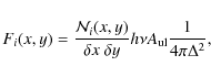
where
We define
![]() to be the number of CO molecules in the upper state of the transition sampled by the cells with Doppler velocities contributing to channel i
to be the number of CO molecules in the upper state of the transition sampled by the cells with Doppler velocities contributing to channel i
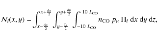 |
(4) |
where pu is the relative population of the upper level of the transition, which depends on the radial distance to nucleus,
![\begin{displaymath}{\rm H}_i(x,y,z) = \left\{
\begin{array}{ll}
1 & \textrm{if...
...v}{2}\right] \\
0 & \textrm{elsewhere}
\end{array}
\right.
\end{displaymath}](/articles/aa/full_html/2009/38/aa11765-09/img109.png) |
(5) |
where vz(x,y,z) is the gas velocity projected onto the line of sight. The gas velocity is radial, and its amplitude is represented by a Gaussian centred on
Because the CO production rate is high in comet Hale-Bopp and a dense CO jet is present, optical depth effects need to be considered when calculating the CO J(2-1) brightness distribution (i.e., Fi(x,y)). They are not expected to affect the ON-OFF spectra significantly, but could be significant in the case of the interferometric signals. The results presented in this paper were performed by solving the full radiative transfer equation, as explained in Boissier et al. (2007), assuming the local velocity dispersion to be thermal.
A synthetic 47-channels ON-OFF spectrum is obtained by the convolution of Fi with the antennas primary beam. For each channel i, the visibilities are defined by (see e.g., Thompson et al. 1991, Chap. 4, Sect. 4.1):
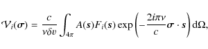
where
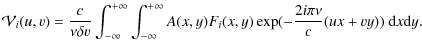 |
(7) |
Visibilities are computed with a Fast Fourier Transform (FFT) algorithm.
The population of the rotational levels (pu) is derived from an
excitation model that takes into account collisions with H2O and
IR radiative pumping of the v(1-0) CO vibrational band
(Crovisier & Le Bourlot 1983; Crovisier 1987). This model describes populations pu as
a function of radial distance r, given a H2O density law with r.
For simplicity, we assumed an isotropic H2O coma, and a pu that only depends upon r. The collisional CO-H2O cross-section is taken to be
equal to
![]() cm2 (Biver et al. 1999b), and the
H2O production rate is
cm2 (Biver et al. 1999b), and the
H2O production rate is
![]() s-1 (Colom et al. 1999). In the simulations presented in Sect. 4, a kinetic temperature T = 120 K is used (see Sect. 2.2
for further discussion). The evolution of the population
of the CO J = 2 and J = 1 levels is shown in Fig. 11.
The beam size of
s-1 (Colom et al. 1999). In the simulations presented in Sect. 4, a kinetic temperature T = 120 K is used (see Sect. 2.2
for further discussion). The evolution of the population
of the CO J = 2 and J = 1 levels is shown in Fig. 11.
The beam size of
![]() for CO J(2-1) corresponds to
for CO J(2-1) corresponds to
![]() km in the coma. Most CO molecules within the
field of view are in local thermal equilibrium.
km in the coma. Most CO molecules within the
field of view are in local thermal equilibrium.
Table 2: Model parameters.
![\begin{figure}
\par\resizebox{9cm}{!}
{\includegraphics[angle=270]{1176511.ps}}
\end{figure}](/articles/aa/full_html/2009/38/aa11765-09/img124.png) |
Figure 11: Relative populations of the CO rotational levels J=1 and J=2, as function of distance from the nucleus. A kinetic temperature of 120 K is assumed. |
| Open with DEXTER | |
Given the evolving coma, a full simulation of the observations
would require to compute for each one minute scan the visibilities
corresponding to the current state of the coma and their
uv-coverage. To limit the computer time, we modelled an
entire nucleus revolution (P = 11.35 h) with
12 snapshots (see Fig. 12). We tested the validity of the
approach by verifying that calculations of higher time sampling
(namely 36 snapshots) provide similar results. Between 2 snapshots i and
i+1, the jet direction changed according to
![]() ,
where
,
where
![]() is the rotation matrix for a time span of
P/12. Provided that the initial jet longitude at time t
corresponding to snapshot i = 1 is fixed, a composite uv-table
can be computed with the uv-coverage of the observations. The
numerical code computes twelve composite uv-tables, each of them
corresponding to different initial jet longitudes at intervals of
360
is the rotation matrix for a time span of
P/12. Provided that the initial jet longitude at time t
corresponding to snapshot i = 1 is fixed, a composite uv-table
can be computed with the uv-coverage of the observations. The
numerical code computes twelve composite uv-tables, each of them
corresponding to different initial jet longitudes at intervals of
360![]() /12. The longitude origin is chosen so that the
sub-terrestrial point on the nucleus surface is at a longitude of
0
/12. The longitude origin is chosen so that the
sub-terrestrial point on the nucleus surface is at a longitude of
0![]() .
For illustration, Fig. 12 shows the twelve jet
positions for a jet at a longitude of 0
.
For illustration, Fig. 12 shows the twelve jet
positions for a jet at a longitude of 0![]() at the time of the
first snapshot. The model also computes synthetic ON-OFF spectra
for each snapshot.
at the time of the
first snapshot. The model also computes synthetic ON-OFF spectra
for each snapshot.
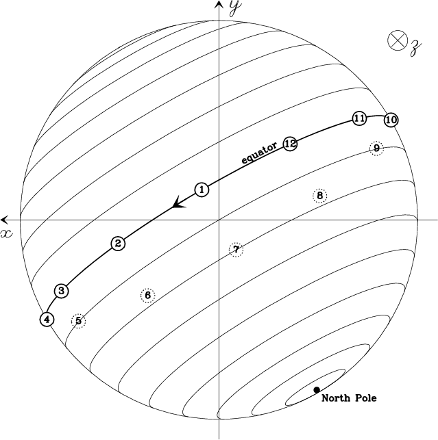 |
Figure 12:
Schematic view of comet Hale-Bopp nucleus on 11 March, 1997,
as seen from the Earth assuming
|
| Open with DEXTER | |
4 Jet morphology analysis
The ON-OFF and interferometric velocity shift
curves observed for CO J(2-1) (Figs. 4
and 10), and the time evolution of the
visibilities (Fig. 9) are now analysed with the model
presented in the previous Section to constrain its free
parameters. Because of the limited signal-to-noise ratio of the data, a
similar analysis was impossible for J(1-0) observations. For the
spin axis orientation defined by its aspect angle
![]() and
position angle
and
position angle
![]() ,
we restricted our study to the mean values
found in the literature (see Table 1):
,
we restricted our study to the mean values
found in the literature (see Table 1):
![]() = 60 to
90
= 60 to
90![]() ,
and
,
and
![]() = 200 to 230
= 200 to 230![]() .
The jet width
.
The jet width ![]() was
tested from 1
was
tested from 1![]() to 90
to 90![]() ,
the jet latitude
,
the jet latitude ![]() from
0
from
0![]() to 90
to 90![]() North, and
North, and
![]() from 10% to 80%.
from 10% to 80%.
4.1 ON-OFF velocity shift curve
![\begin{figure}
\par\resizebox{9cm}{!}
{\includegraphics[angle=270]{1176513.ps}}
\end{figure}](/articles/aa/full_html/2009/38/aa11765-09/img128.png) |
Figure 13:
Evolution of the amplitude of the velocity shift curve
|
| Open with DEXTER | |
As discussed in Sect. 2.2, data shown in Fig. 4
are well fitted by a sinusoid with a period P=11.35 h, an amplitude
![]() km s-1, and centred on v0=-0.05 km s-1. We can also define a phase
km s-1, and centred on v0=-0.05 km s-1. We can also define a phase
![]() UT, which corresponds to the time when the velocity shift
is equal to v0 on the increasing side of the curve.
We used these three parameters (
UT, which corresponds to the time when the velocity shift
is equal to v0 on the increasing side of the curve.
We used these three parameters (
![]() ,
v0, t0) as
criteria when selecting the models that could explain the observations.
We note that the position angle
,
v0, t0) as
criteria when selecting the models that could explain the observations.
We note that the position angle
![]() of the spin axis
has no influence on the velocity shift.
of the spin axis
has no influence on the velocity shift.
The phase t0 is controlled only by the initial longitude of the jet. From t0 derived from the observations, we infer the initial longitude to be 300![]() at 3 h 47 UT.
at 3 h 47 UT.
To first order,
![]() is governed by
is governed by
![]() and
and ![]() : it increases when either
: it increases when either
![]() increases or
increases or ![]() decreases. This behaviour can be easily explained. If
decreases. This behaviour can be easily explained. If
![]() increases - all other parameters remaining unchanged - more signal
from the jet falls into the same number of spectral channels.
The velocity shift and the amplitude of the velocity shift curve then increase. In a similar way, when
increases - all other parameters remaining unchanged - more signal
from the jet falls into the same number of spectral channels.
The velocity shift and the amplitude of the velocity shift curve then increase. In a similar way, when ![]() decreases - keeping
decreases - keeping
![]() constant - an equal amount of signal coming from the jet covers a larger number of spectral channels. This results in reducing both the velocity shift and
constant - an equal amount of signal coming from the jet covers a larger number of spectral channels. This results in reducing both the velocity shift and
![]() .
This is illustrated in Figs. 13 and 14,
which show the evolution in
.
This is illustrated in Figs. 13 and 14,
which show the evolution in
![]() with
with
![]() and
and ![]() .
Moreover,
.
Moreover,
![]() is
insensitive to the aspect angle
is
insensitive to the aspect angle
![]() ,
except for small
,
except for small ![]() 's, as observed in Figs. 13 and 14. Furthermore, we note that the jet latitude
's, as observed in Figs. 13 and 14. Furthermore, we note that the jet latitude ![]() has little
influence on the amplitude, within the limits that we tested (
has little
influence on the amplitude, within the limits that we tested (![]()
![]() )
(Fig. 15).
To conclude, the observed amplitude of 0.29 km s-1 can be fitted by many (
)
(Fig. 15).
To conclude, the observed amplitude of 0.29 km s-1 can be fitted by many (
![]() ,
,![]() ,
,![]() )
combinations.
)
combinations.
![\begin{figure}
\par\resizebox{9cm}{!}
{\includegraphics[angle=270]{1176514.ps}}
\end{figure}](/articles/aa/full_html/2009/38/aa11765-09/img132.png) |
Figure 14:
Evolution of the amplitude of the velocity shift curve
|
| Open with DEXTER | |
![\begin{figure}
\par\resizebox{9cm}{!}{
\includegraphics[angle=270]{1176515a.ps}}...
...2cm}
\resizebox{9cm}{!}{\includegraphics[angle=270]{1176515b.ps}}
\end{figure}](/articles/aa/full_html/2009/38/aa11765-09/img133.png) |
Figure 15:
Evolution of
|
| Open with DEXTER | |
The mean velocity v0 of the simulated curves depends mainly on the jet latitude ![]() .
An equatorial jet always produces a curve centred on 0 km s-1, regardless
.
An equatorial jet always produces a curve centred on 0 km s-1, regardless
![]() .
For
.
For
![]() < 90
< 90![]() ,
a
jet with a northern (respectively southern) latitude produces a curve centred on a negative (respectively positive) velocity. This behaviour is again understandable. With
,
a
jet with a northern (respectively southern) latitude produces a curve centred on a negative (respectively positive) velocity. This behaviour is again understandable. With
![]() < 90
< 90![]() ,
the North pole is pointing towards the Earth (see Fig. 12). As a result, a northern jet is directed towards the Earth for a longer time than a southern one. The opposite effects are obtained for
,
the North pole is pointing towards the Earth (see Fig. 12). As a result, a northern jet is directed towards the Earth for a longer time than a southern one. The opposite effects are obtained for
![]() > 90
> 90![]() ,
while
,
while
![]() = 90
= 90![]() (rotation axis in the plane of the sky) always produces a curve
centred on 0 km s-1, irrespective of the sign of the latitude.
The greater the rotation axis is from the plane of the sky, the greater the shift in the velocity shift curve. Furthermore, the velocity shift curve is shifted all the more because
(rotation axis in the plane of the sky) always produces a curve
centred on 0 km s-1, irrespective of the sign of the latitude.
The greater the rotation axis is from the plane of the sky, the greater the shift in the velocity shift curve. Furthermore, the velocity shift curve is shifted all the more because ![]() is small and
is small and
![]() is large (Fig. 15).
This study leads us to the conclusion that, here again, many combinations (
is large (Fig. 15).
This study leads us to the conclusion that, here again, many combinations (
![]() ,
,![]() ,
,![]() )
are able to reproduce the observed v0. However, it shows that only a
northern jet can describe the observations.
)
are able to reproduce the observed v0. However, it shows that only a
northern jet can describe the observations.
![\begin{figure}
\par\includegraphics[angle=270,width=17cm]{1176516.ps}
\end{figure}](/articles/aa/full_html/2009/38/aa11765-09/img134.png) |
Figure 16:
The pairs of parameters (
|
| Open with DEXTER | |
For a given (
![]() ,
,![]() ,
,
![]() )
parameter set, it is possible to
find the jet width
)
parameter set, it is possible to
find the jet width ![]() that is able to reproduce the amplitude
that is able to reproduce the amplitude
![]() km s-1. Figure 16 shows in dotted curves the locus of the pairs (
km s-1. Figure 16 shows in dotted curves the locus of the pairs (
![]() ,
,![]() )
that reproduce the correct amplitude
)
that reproduce the correct amplitude
![]() for several fixed (
for several fixed (
![]() ,
,![]() )
values. The same method is employed to determine the pairs of
variables (
)
values. The same method is employed to determine the pairs of
variables (
![]() ,
,![]() )
that reproduce the correct velocity centre
v0 = -0.05 km s-1 (dashed curves in
Fig. 16). For each set (
)
that reproduce the correct velocity centre
v0 = -0.05 km s-1 (dashed curves in
Fig. 16). For each set (
![]() ,
,![]() ), the
intersection of the dotted and the dashed curves infers the only pair (
), the
intersection of the dotted and the dashed curves infers the only pair (
![]() ,
,![]() )
that reproduces
)
that reproduces
![]() and v0. We completed these computations for latitudes of between 0
and v0. We completed these computations for latitudes of between 0![]() and 45
and 45![]() ,
and for
,
and for
![]() = 70
= 70![]() and 80
and 80![]() .
Computations for
.
Computations for
![]() = 90
= 90![]() were useless because they infer that v0=0 km s-1.
were useless because they infer that v0=0 km s-1.
The combinations (
![]() ,
,
![]() ,
,![]() ,
,![]() )
selected by this study are summarized in Table 3. We note that the jet strength
)
selected by this study are summarized in Table 3. We note that the jet strength
![]() is typically between 35% and 50%. The jet is located on the northern hemisphere at a latitude
of between 0
is typically between 35% and 50%. The jet is located on the northern hemisphere at a latitude
of between 0![]() and 45
and 45![]() (both excluded) for
(both excluded) for
![]() = 80
= 80![]() ,
and between 0
,
and between 0![]() and 20
and 20![]() (both excluded) for
(both excluded) for
![]() = 70
= 70![]() .
.
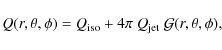
The velocity shift curve obtained for parameter set (3) is shown in Fig. 10, together with the observed curve. We note the almost perfect match between model and observations. The corresponding synthetic line profiles are shown in Fig. 17. At any time, the jet contributes to both blue and red channels, their relative contributions varying because of its spiral shape.
Table 3:
Selected sets of parameters
![]() ,
,
![]() ,
,
![]() and
and
![]() reproducing the velocity shift curve of the ON-OFF observations.
reproducing the velocity shift curve of the ON-OFF observations.
![\begin{figure}
\par\includegraphics[angle=-90,width=7.5cm,clip]{1176517.ps}
\end{figure}](/articles/aa/full_html/2009/38/aa11765-09/img135.png) |
Figure 17:
Synthetic CO 230 GHz ON-OFF line profile as a function of UT time on 11 March for parameter set (3) of
Table 3 (
|
| Open with DEXTER | |
4.2 Interferometric velocity shift curves
We now study the velocity shift curves observed for
the individual baselines. Figure 10 shows
model results for the parameter set (3) in Table 3 (i.e.,
![]() = 80
= 80![]() ,
,
![]() = 210
= 210![]() ,
,
![]() = 18.3
= 18.3![]() ,
,
![]() = 20
= 20![]() and
and
![]() = 35.5%). Other parameter sets
in Table 3 produce similar curves. Modelled
curves are periodic functions, with a period equal to P. They
mimic sinusoidal curves, although significant deviations from a
sinusoid are observed. This is because line shifts measured in
= 35.5%). Other parameter sets
in Table 3 produce similar curves. Modelled
curves are periodic functions, with a period equal to P. They
mimic sinusoidal curves, although significant deviations from a
sinusoid are observed. This is because line shifts measured in
![]() spectra are (u,v) dependent: stronger jet
contrast appears in specific regions because of spatial filtering.
Then, because of the combination of Earth and jet rotation, regions
with more or less jet contrast are sampled by the individual
baselines. Simulations indicate that these curves evolve toward a true
sinusoid when the jet width
spectra are (u,v) dependent: stronger jet
contrast appears in specific regions because of spatial filtering.
Then, because of the combination of Earth and jet rotation, regions
with more or less jet contrast are sampled by the individual
baselines. Simulations indicate that these curves evolve toward a true
sinusoid when the jet width ![]() is increasing (
is increasing (
![]() kept
constant), due to smaller jet contrast. These curves change when
varying the jet parameters in the same way as for the ON-OFF
curve. Changing the spin axis parameters by
kept
constant), due to smaller jet contrast. These curves change when
varying the jet parameters in the same way as for the ON-OFF
curve. Changing the spin axis parameters by ![]() 10
10![]() does
not significantly affect the curves.
does
not significantly affect the curves.
![\begin{figure}
\par\resizebox{9cm}{!}{\includegraphics[bb=60 43 536 690,clip=true]{1176518.ps}}
\end{figure}](/articles/aa/full_html/2009/38/aa11765-09/img138.png) |
Figure 18:
Phase t0 ( bottom) and amplitude
|
| Open with DEXTER | |
The modelled velocity shift curves for the different baselines are
not in phase, t0 (defining the phase, see
Sect 4.1) increasing with decreasing baseline length
(Fig. 18). We expect a phase offset because of
the spiral shape of the jet. With respect to long baselines,
short baselines probe molecules in more distant regions of
the spiral. Hence, they sample molecules released on average at
earlier times. In addition, baselines of different
length (even if they are parallel) detect the maximum amount of signal from the jet at different times due to the curvature of the jet. This can be understood from Fig. 19, which plots the amplitude of the visibility as a function of both the orientation and length of the baselines for
a simple geometry (rotation axis along the line of sight and
equatorial jet) and at a given time. The combination of both effects
introduces a phase offset in the velocity shift curves.
The delay between two baselines in the
velocity shift curves represents the elapsed time between the jet
detection by one baseline and its detection by the following one.
We note that, given the large curvature of the
spiral (molecules travel
![]() km, when the nucleus
rotates by 90
km, when the nucleus
rotates by 90![]() ), only its innermost part contributes
significantly to the detected signal. The dashed curve in
Fig. 18 shows the evolution of t0 with
uv-radius, assuming that t0 varies linearly with
), only its innermost part contributes
significantly to the detected signal. The dashed curve in
Fig. 18 shows the evolution of t0 with
uv-radius, assuming that t0 varies linearly with
![]() /
/![]() ,
which agrees approximately with the t0 curve
computed by the model (plain curve).
,
which agrees approximately with the t0 curve
computed by the model (plain curve).
![\begin{figure}
\par\resizebox{9cm}{!} {\includegraphics[angle=270,width=6cm,clip=true]{1176519.ps}}
\end{figure}](/articles/aa/full_html/2009/38/aa11765-09/img141.png) |
Figure 19:
Visibilities of the CO 230 GHz line (central chanel) as a
function of baseline orientation in the uv plane and baseline length ( |
| Open with DEXTER | |
The comparison between modelled and observed phases t0 and
amplitudes
![]() shows that there is relatively good agreement for
some baselines and strong discrepancies for others
(Fig. 18). Good agreement for both t0 and
shows that there is relatively good agreement for
some baselines and strong discrepancies for others
(Fig. 18). Good agreement for both t0 and
![]() is obtained for baselines 3-4 and 2-4. Phase t0 is well
reproduced for baseline 1-3 (but not amplitude). A strong
discrepancy (of 3 h for t0, and a factor of almost 2 for
is obtained for baselines 3-4 and 2-4. Phase t0 is well
reproduced for baseline 1-3 (but not amplitude). A strong
discrepancy (of 3 h for t0, and a factor of almost 2 for
![]() )
is
observed for baselines 1-4, 1-5, and possibly 4-5 (errorbars are
large for this baseline). It is remarkable that good
agreement is obtained for baselines of field of view
aligned along the spin vector, while discrepancies are observed
for baselines of field of view perpendicular to the spin
vector. Clearly our model is too simple to reproduce all
observational characteristics. We were unable to identify any simple
explanation of these discrepancies. Velocity acceleration inside
the jet would change the t0 evolution with baseline in an opposite way:
it would produce a flatter increase with decreasing baseline
length than obtained with a constant velocity. The presence of
other CO evolving structures in the coma of Hale-Bopp is, however, the most likely explanation (Sect. 4.5).
)
is
observed for baselines 1-4, 1-5, and possibly 4-5 (errorbars are
large for this baseline). It is remarkable that good
agreement is obtained for baselines of field of view
aligned along the spin vector, while discrepancies are observed
for baselines of field of view perpendicular to the spin
vector. Clearly our model is too simple to reproduce all
observational characteristics. We were unable to identify any simple
explanation of these discrepancies. Velocity acceleration inside
the jet would change the t0 evolution with baseline in an opposite way:
it would produce a flatter increase with decreasing baseline
length than obtained with a constant velocity. The presence of
other CO evolving structures in the coma of Hale-Bopp is, however, the most likely explanation (Sect. 4.5).
4.3 Visibilities
Figure 9 shows the time evolution in the
visibilities
![]() plotted as a function of the uv-radius
plotted as a function of the uv-radius
![]() (as defined in Sect. 2.3,
(as defined in Sect. 2.3,
![]() refers to
the amplitude of the visibilities integrated over velocity). A
least squares fit to these data implies that
refers to
the amplitude of the visibilities integrated over velocity). A
least squares fit to these data implies that
![]() ,
which should be compared with the
,
which should be compared with the
![]() variation expected for a parent molecule
distribution and an optically thin line (Bockelée-Morvan & Boissier 2009).
This trend can be explained by optical depth effects being more important for long baselines probing the inner coma.
variation expected for a parent molecule
distribution and an optically thin line (Bockelée-Morvan & Boissier 2009).
This trend can be explained by optical depth effects being more important for long baselines probing the inner coma.
Modulations are observed about this fit: they trace variations
in the brightness distribution sampled by the individual baselines as the baselines and jet rotate. These modulations are characterized by both their shape and amplitude. Their shape depends on the rotation-axis position angle
![]() and the jet latitude
and the jet latitude ![]() .
For example, a high-latitude jet would
result in strong modulations for baselines 3-4, 2-4, and 2-3, and
no modulations for baselines 1-3 and 1-4, which scan regions along the equator (Fig. 20). The reverse is expected for
a high-latitude jet and a
.
For example, a high-latitude jet would
result in strong modulations for baselines 3-4, 2-4, and 2-3, and
no modulations for baselines 1-3 and 1-4, which scan regions along the equator (Fig. 20). The reverse is expected for
a high-latitude jet and a
![]() of 90
of 90![]() from the nominal
from the nominal
![]() of the Hale-Bopp rotation axis. Qualitatively, the observed modulations exclude both a high-latitude jet and a rotation-axis position angle that differs much from the
of the Hale-Bopp rotation axis. Qualitatively, the observed modulations exclude both a high-latitude jet and a rotation-axis position angle that differs much from the
![]() derived from visible observations. This confirms the conclusion obtained from the time evolution of the photometric centres (Sect. 2.3), which is
sensitive to both the amplitude and phase of the visibilities.
derived from visible observations. This confirms the conclusion obtained from the time evolution of the photometric centres (Sect. 2.3), which is
sensitive to both the amplitude and phase of the visibilities.
![\begin{figure}
\par\resizebox{9cm}{!}{\includegraphics[angle=270]{1176520.ps}}
\end{figure}](/articles/aa/full_html/2009/38/aa11765-09/img144.png) |
Figure 20: CO 230 GHz modelled visibilities for a high-latitude jet. |
| Open with DEXTER | |
![\begin{figure}
\par\resizebox{9cm}{!}
{\includegraphics[angle=270]{1176521.ps}}
\end{figure}](/articles/aa/full_html/2009/38/aa11765-09/img145.png) |
Figure 21:
CO 230 GHz modelled visibilities for the jet and rotation axis parameters which reproduce at best the observations (set (3) with
|
| Open with DEXTER | |
![\begin{figure}
\par\resizebox{9cm}{!}
{\includegraphics[angle=270]{1176522.ps}}
\end{figure}](/articles/aa/full_html/2009/38/aa11765-09/img146.png) |
Figure 22:
CO 230 GHz modelled visibilities for set (3) with
|
| Open with DEXTER | |
We compared the observed visibilities to those computed by the
model with the sets of jet parameters (2), (3), and (4) given in
Table 3 (those with
![]() = 80
= 80![]() and
and
![]() = 210
= 210![]() ). The lowest
). The lowest ![]() (reduced
(reduced
![]() = 5.1
for N = 150 data points and n = 5 free parameters) was obtained for the set of parameters (3) with
= 5.1
for N = 150 data points and n = 5 free parameters) was obtained for the set of parameters (3) with
![]()
![]() ,
,
![]() = 20
= 20![]() ,
and
,
and
![]() = 35.5%. Simulations with the parameter set (2) (respectively (4))
show larger (respectively lower) modulations than observed, and
= 35.5%. Simulations with the parameter set (2) (respectively (4))
show larger (respectively lower) modulations than observed, and ![]() values 60% (respectively 22%) larger than with parameters (3). Using
the jet parameter set (3), we also compiled simulations with
values 60% (respectively 22%) larger than with parameters (3). Using
the jet parameter set (3), we also compiled simulations with
![]() = 60 and
70
= 60 and
70![]() ,
and
,
and
![]() = 200, 220, and 230
= 200, 220, and 230![]() .
The
.
The ![]() was
minimized for
was
minimized for
![]() = 220
= 220![]() (
(
![]() ), while
), while
![]() has no
significant influence on the visibilities. However,
has no
significant influence on the visibilities. However,
![]() = 210
= 210![]() provides a solution that explains the visibilities of the 3-4 baseline more accurately. Figure 21 shows the modelled visibilities
with parameters (3) and
provides a solution that explains the visibilities of the 3-4 baseline more accurately. Figure 21 shows the modelled visibilities
with parameters (3) and
![]() = 210
= 210![]() .
Looking at the shape
of the modulations, there is overall agreement between model and
observations, although the agreement is not perfect. A
plot of observed versus modelled visibilities shows that the closest
agreement is for baselines 3-4, 1-5, 1-4, 1-3, and 4-5. The
largest discrepancies are for baselines 2-4, 1-2, and 2-5. For
most baselines, jet detection (traced by amplitude increase)
occurs
.
Looking at the shape
of the modulations, there is overall agreement between model and
observations, although the agreement is not perfect. A
plot of observed versus modelled visibilities shows that the closest
agreement is for baselines 3-4, 1-5, 1-4, 1-3, and 4-5. The
largest discrepancies are for baselines 2-4, 1-2, and 2-5. For
most baselines, jet detection (traced by amplitude increase)
occurs ![]() 1 h earlier in the simulation than in the
observations. In contrast, in the velocity shift curves, the
simulated jet is late with respect to the observed jet for most
baselines. This again shows that our model is too simple to
explain the data satisfactorily.
1 h earlier in the simulation than in the
observations. In contrast, in the velocity shift curves, the
simulated jet is late with respect to the observed jet for most
baselines. This again shows that our model is too simple to
explain the data satisfactorily.
The visibilities obtained when optical depth effects are neglected, exhibit the same temporal behaviour (Fig. 22). However, as expected, the modulations are more prominent in the optically thin case.
The visibilities obtained with jet parameter set (3) vary according to
![]() ,
which is
consistent, to first order, with the observed variation
(
,
which is
consistent, to first order, with the observed variation
(
![]() ).
).
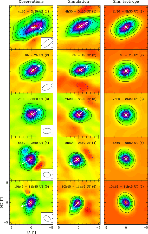 |
Figure 23:
CO 230 GHz Hale-Bopp maps as a function of time. Left column: observations; central column: simulations with the jet and rotation axis parameters that reproduce most effectively the observations (set (3):
|
| Open with DEXTER | |
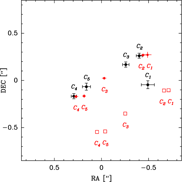 |
Figure 24:
Time evolution of the photometric centre, determined
by fitting data in the uv-plane. Measurements for Hale-Bopp
CO 230 GHz observations are shown by black dots with errorbars. Those
from simulations with jet parameter set (3) (
|
| Open with DEXTER | |
4.4 Maps
Simulated maps as a function of time are compared with observed maps in
Fig. 23. The shape of the observed CO coma is relatively
well reproduced by the model. Some differences may be caused by the presence
of other CO coma features, as suggested by noticeable discrepancies at
8h50-9h5 UT. The time evolution of
the photometric centre measured in the simulated data (jet parameters (3) with
![]() = 210
= 210![]() )
is shown in
Fig. 24. When the position of
the photometric centre is defined with respect to the mean photometric
centre for the observing period, and can therefore be directly
compared to the measurements, there is good agreement in the overall
evolution. As expected, the relative
(modelled-observed) positions generally differ, with discrepancies reaching
)
is shown in
Fig. 24. When the position of
the photometric centre is defined with respect to the mean photometric
centre for the observing period, and can therefore be directly
compared to the measurements, there is good agreement in the overall
evolution. As expected, the relative
(modelled-observed) positions generally differ, with discrepancies reaching ![]() 0.3
0.3
![]() for 4h30-5h30 and 7h20-8h20 data (maps 1 and 3).
However, the good overall agreement confirms a posteriori that the
observed time evolution of the CO 230 GHz peak brightness position is related to the CO rotating coma.
for 4h30-5h30 and 7h20-8h20 data (maps 1 and 3).
However, the good overall agreement confirms a posteriori that the
observed time evolution of the CO 230 GHz peak brightness position is related to the CO rotating coma.
We compiled synthetic 230 GHz spectral maps that are directly comparable to the observations (Fig. 6). Some observed basic features are well reproduced, such as the very peaked and strong emission in the blue channels at high velocity and the elongated coma in the East-West direction for the blue channels at velocities close to zero. However, the asymmetry in the spatial distribution observed in the red channels is not reproduced by the model. As a matter of fact, the model, whose parameters were constrained by the large-scale ON-OFF observations, predicts that the inner parts of the jet probed during the course of the interferometric observations were most of the time projecting Earthward (i.e., with negative Doppler velocities). The discrepancies between modelled and observed spectral visibilities discussed previously are observed directly on the spectral maps.
4.5 Evidence of a second moving structure
![\begin{figure}
\par {\includegraphics[angle=270,width=17cm]{1176525a.ps} }
\par {\includegraphics[angle=270,width=17cm]{1176525b.ps} }
\end{figure}](/articles/aa/full_html/2009/38/aa11765-09/img155.png) |
Figure 25: Time evolution of the CO 230 GHz photometric centre for individual velocity channels at v = -1.0, -0.5, 0, +0.5, +1.0 km s-1. The spectral data were smoothed to a spectral resolution of 0.5 km s-1. The time intervals labelled 1 to 6 are given in Sect. 4.5 . Note that they do not correspond to those used for Figs. 23 and 24. The top figure shows the measurements, while the model (set of parameters (3) in Table 3) is shown in the bottom figure. To illustrate how the photometric centres are affected by the main jet, we have connected points (coloured in blue) indicative of the motion of the CO main jet. The so-called ''red jet'' is shown by red symbols. |
| Open with DEXTER | |
The inability of our one-jet model to reproduce satisfactorily the interferometric data is due to the presence of a second moving CO structure, possibly produced during an outburst.
This moving structure is that seen North-West from the nucleus at positive velocities in the time-averaged channel maps (Fig. 6). This structure, which is moving away from the observer, is oriented along the fringes of baselines 1-4, 1-5, 3-5, and 4-5, i.e., along those for which a strong discrepancy in the time variation of the velocity shift is observed. This structure is clearly detected by these baselines : hence, the velocity shift measured for these baselines is smaller than expected (Fig. 10).
To study the time evolution of this stucture, the spectral data were smoothed to a spectral resolution of 0.5 km s-1, for velocity channels centred on -1.0, -0.5, 0, +0.5,
+1.0 km s-1 with respect to the comet rest velocity. Five
consecutive time intervals (![]() ,
,
![]() 2,
2, ![]() 4,
4, ![]() 5,
5, ![]() 6) of
between
6) of
between ![]() 50 min and 1h30 long, were considered. The time intervals
correspond to characteristic line shapes in the spectrum recorded
by baseline 3-4 (Fig. 3):
50 min and 1h30 long, were considered. The time intervals
correspond to characteristic line shapes in the spectrum recorded
by baseline 3-4 (Fig. 3): ![]() (4h30-5h48 UT) symmetric shape ;
(4h30-5h48 UT) symmetric shape ; ![]() 2 ( 5h48-7h07 UT) and
2 ( 5h48-7h07 UT) and ![]() 4 (7h07-9h08 UT) asymmetric shape with strong blueshift ;
4 (7h07-9h08 UT) asymmetric shape with strong blueshift ; ![]() 5 (9h08-10h00 UT) symmetric shape; and
5 (9h08-10h00 UT) symmetric shape; and ![]() 6 (10h00 UT-11h28) asymmetric shape with high redshift. A sixth period, labelled
6 (10h00 UT-11h28) asymmetric shape with high redshift. A sixth period, labelled ![]() 3, merging intervals
3, merging intervals ![]() 2 and
2 and ![]() 4, was also considered.
4, was also considered.
The
![]() extracted data sets were analysed in the Fourier
plane by assuming that the brightness distribution is a 2D Gaussian,
and that its intensity, width and offset with respect to the
line-integrated, time-averaged centre Cm were free parameters.
Figure 25 shows the observed time evolution of the
offset (RA(t), Dec(t)) for each channel. The same plot is shown
using model parameter set (3) as input.
extracted data sets were analysed in the Fourier
plane by assuming that the brightness distribution is a 2D Gaussian,
and that its intensity, width and offset with respect to the
line-integrated, time-averaged centre Cm were free parameters.
Figure 25 shows the observed time evolution of the
offset (RA(t), Dec(t)) for each channel. The same plot is shown
using model parameter set (3) as input.
For a non-rotating nucleus, the motion of a cloud of gas released
during a short time interval from a nuclear source should follow
a straight line in the (RA, Dec) quadrant and the velocity
channel where its velocity vector is projected. For a rotating
nucleus, a permanent nuclear source near the equator will produce
an expanding jet that will appear successively in the different
channels as the nucleus rotates. In the case of comet Hale-Bopp,
if the equatorial jet projects North-West in (RA, Dec) at positive
velocity channels (V+) at a given time, then it will
project North-West in negative velocity channels
(V-), South-East/V-, South-East/V+. As shown in
Fig. 25, there is satisfactory agreement between
model and observations for channels centred on -1.0,
-0.5 and 0 km s-1. We tentatively connected the points
corresponding to the motion of the CO main jet. At time ![]() ,
the
jet is moving westward in the v = 0 channel; at time
,
the
jet is moving westward in the v = 0 channel; at time ![]() 4, it is moving
eastward in the v = -0.5 km s-1 channel; at time
4, it is moving
eastward in the v = -0.5 km s-1 channel; at time ![]() 5,
eastward in the v = 0 channel; and at time
5,
eastward in the v = 0 channel; and at time ![]() 6, eastward in the
v = +0.5 km s-1 channel.
6, eastward in the
v = +0.5 km s-1 channel.
The motion of the red structure is clearly apparent in the
channels at v = +0.5 and +1 km s-1. The direction of the
motion suggests that it originates in a low latitude region at
the nucleus surface. The longitude of this source is estimated to
be within 90-150![]() westward from the source of the main
jet. The weak contribution of the red structure to some baselines
can be explained by spatial filtering, implying that a compact
structure is present. The CO 230 GHz flux density in channels v = +0.5 and
+1 km s-1 is four times lower than in channel v = -0.5 km s-1, at the time that the CO main jet is contributing. This may
explain why the red source does not contribute much to the ON-OFF
spectra.
westward from the source of the main
jet. The weak contribution of the red structure to some baselines
can be explained by spatial filtering, implying that a compact
structure is present. The CO 230 GHz flux density in channels v = +0.5 and
+1 km s-1 is four times lower than in channel v = -0.5 km s-1, at the time that the CO main jet is contributing. This may
explain why the red source does not contribute much to the ON-OFF
spectra.
5 Discussion
5.1 Model assumptions
The observations presented in this paper have been interpreted with a
simple geometric model of a CO rotating coma. Apart from the assumed
conical shape of the jet at ejection (see the discussion below), several other
simplifying assumptions were made to limit the number of free
model parameters. The outflow velocity was fixed and taken to be
constant throughout the coma, whereas some acceleration is
expected by gas dynamical models (Combi et al. 1999). Day-to-night
asymmetries in velocity for the CO background gas were not taken
into account, although they are clearly present. The
velocity cutoff and width of the blue wing of the CO velocity
profiles are indeed 10% higher than the corresponding values for the red
wings (Fig. 3), which suggests higher velocities
towards the sunlit side of the nucleus given the Earth-comet-Sun
geometry. In addition, we assumed that CO molecules inside the jet
expand at the same velocity as those in the background. We
believe that including slight variations in the flow velocity
field would not change the main conclusions of this paper, although
the characteristics of the jet could somewhat differ. For example,
including the day-to-night asymmetry in velocity would shift the
jet towards lower latitudes. Higher velocities inside the jet
would require a proportionally higher jet contribution to the
total CO production
![]() to fit the ON-OFF data. We also did not
consider the temperature variations in the coma that can have
direct effects on CO excitation. A kinetic temperature that is higher in
the jet than in the background gas would have resulted in a higher
inferred
to fit the ON-OFF data. We also did not
consider the temperature variations in the coma that can have
direct effects on CO excitation. A kinetic temperature that is higher in
the jet than in the background gas would have resulted in a higher
inferred
![]() .
However, a 10 K difference in temperature would
change
.
However, a 10 K difference in temperature would
change
![]() by less than 10%.
by less than 10%.
5.2 CO jet
Our observations, interpreted with the help of a simple model,
suggest the presence of a spiralling ``jet'' of CO, originating in the
nucleus. The rotation of this jet is consistent with the rotation
period and axis direction derived from most optical studies. The jet
originates in a low-latitude (![]() 20
20![]() )
region of the nucleus, and
is responsible for a significant amount of the total CO production (
)
region of the nucleus, and
is responsible for a significant amount of the total CO production (![]() 40%) in a
40%) in a ![]() 20-30
20-30![]() wide
aperture. This is the first evidence of a CO spiralling coma around a comet nucleus. The CO ro-vibrational line emission observed in comet Hale-Bopp from January to May 1997 exhibits strong
East/West asymmetries, the position of the maximum brightness
moving with time from up to
wide
aperture. This is the first evidence of a CO spiralling coma around a comet nucleus. The CO ro-vibrational line emission observed in comet Hale-Bopp from January to May 1997 exhibits strong
East/West asymmetries, the position of the maximum brightness
moving with time from up to
![]() 2
2
![]() West to
West to ![]() 2
2
![]() East of the continuum peak (DiSanti et al. 2001; Brooke et al. 2003). This is probably caused by the rotating CO structure observed in the radio (Brooke et al. 2003) and shows that
this CO structure is not a transient phenomenon related to some outburst.
East of the continuum peak (DiSanti et al. 2001; Brooke et al. 2003). This is probably caused by the rotating CO structure observed in the radio (Brooke et al. 2003) and shows that
this CO structure is not a transient phenomenon related to some outburst.
Our model, which includes a single jet, appears to be too simple to interpret all the observational characteristics. Other ``jets'' are present, in particular another moving structure has been identified at positive velocities in the interferometric data. Its full characterization is difficult on the basis of our data and beyond the scope of this paper. The CO main jet is certainly more complex than a simple conical spiralling structure. Gas structures created by inhomogeneities in gas production at the nucleus surface will unescapably be modified during their outflow by the surrounding collisional environment (the collisional sphere in Hale-bopp coma exceeded 105 km near perihelion, Combi et al. 1999).
Gas dynamical models investigating the behavior of expanding dusty gas jets have been developed (see the review of Crifo et al. 2005). One or several active sources releasing water were considered, the remainder of the nucleus being assumed to be weakly active. They show that, because of lateral expansion driven by pressure gradients, jets broaden with increasing distance to nucleus, and interact with each other, to become eventually almost indiscernible in the outer coma. In addition, if there is solar modulation of the surface gas flux, the jet morphology will change its appearance as the nucleus rotates. These calculations may not however be relevant to the CO jet seen in comet Hale-Bopp. First of all, it is very likely that CO diffuses from subsurface layers. Our observations suggest that, to first order, there is no significant day-to-night asymmetry in the amount of CO gas released by the active source. Secondly, if the active source responsible for the CO jet does not produce similarly strong enhancement in water production, pressure smoothing will not be very effective and jet broadening may be produced instead by molecular diffusion. In this case, it is possible that a nearly invariant CO density pattern corotates with the nucleus and remains relatively well preserved on large scales in the coma. However, it can be anticipated that the jet development will still be influenced by the surrounding environment.
A good illustration is the following. Rodionov & Crifo (2006) performed time-dependent 3D gas dynamical calculations by simulating rotationally-induced gas coma structures. They used an arbitrarily Halley-like aspherical nucleus, scaled to the Hale-Bopp nucleus size and homogeneous in composition. Carbon monoxide was assumed to diffuse uniformly from below the surface, and H2O sublimates according to solar illumination. The computed CO coma was asymmetric. The model output has faint H2O and CO spiralling structures resulting from weak shocks induced by the surface topography. In other words, the CO outflow is largely influenced by the general and detailed properties of the flow. The analysis of the CO Plateau de Bure observations using time-dependent (multi-fluid) gas dynamics calculations was performed by Boissier et al. (2005,2009). They show that the observed time variations cannot be explained by the above mentioned shock structures, and are instead caused by a strong inhomogeneity in CO production from the nucleus surface or subsurface. Many hypotheses can explain this CO overproduction. It can traduce inhomogeneities in CO content inside the nucleus but also local variations in mantle thickness, or in some properties of the nucleus material (e.g., dust/ice matrix structure, thermal conductivity). We leave this discussion to experts and encourage them to perform numerical simulations (see the review of Prialnik et al. 2005).
5.3 Comparison with other studies
There are two open questions about our study:
- 1)
- is the CO jet that we observed related (correlated) to jets observed for other molecules?
- 2)
- is the CO jet that we observed related (correlated) to observed dust jets?
Lederer & Campins (2002) and Lederer et al. (2009) observed spiralling jets of OH, CN and C2.
Several (up to five) active areas were necessary to reproduce
their observations from their Monte Carlo simulation. The
strongest jets originate in low-latitude regions (-22![]() to +20
to +20![]() ). One of them could thus be associated with our CO
jet. One low-latitude southern area is responsible for one-half of
the OH coming from jet-source, but has a large opening angle
(120
). One of them could thus be associated with our CO
jet. One low-latitude southern area is responsible for one-half of
the OH coming from jet-source, but has a large opening angle
(120![]() ), so is unlikely to be related to the CO jet. Spatial
profiles of H2O obtained from long-slit observations of
infrared water lines only show small East-West asymmetries
(Dello Russo et al. 2000). In summary, there is no strong evidence of a
strong H2O jet associated with the CO jet.
), so is unlikely to be related to the CO jet. Spatial
profiles of H2O obtained from long-slit observations of
infrared water lines only show small East-West asymmetries
(Dello Russo et al. 2000). In summary, there is no strong evidence of a
strong H2O jet associated with the CO jet.
Woodney et al. (2002) mapped HCN in comet Hale-Bopp with the BIMA array. Their observations, which spanned over several days, were binned and averaged according to the phase of the comet rotation, to avoid smearing due to rotation. They found a jet morphology, possibly correlated with CN imaged in the visible. However, there is apparently no correlation of the HCN with dust jets. The presence of a high-latitude HCN jet is however inferred by the PdBI data (Boissier et al. 2007).
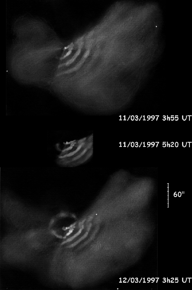 |
Figure 26: Drawings of the inner coma of comet Hale-Bopp on 11 and 12 March, 1997 (N. Biver, 25.6 cm Newtonian telescope). |
| Open with DEXTER | |
Dust jets also appear to be uncorrelated with our CO jet.
From visible imaging at the time of the PdBI observations,
Jorda et al. (1999) observed a high latitude (64![]() )
dust jet. In
the analysis of Vasundhara & Chakraborty (1999), strong dust jets are present from
latitudes +65
)
dust jet. In
the analysis of Vasundhara & Chakraborty (1999), strong dust jets are present from
latitudes +65![]() and -65
and -65![]() ,
in addition to weaker jets from
low latitudes (see also Schleicher et al. 2004). In February-May 1997,
the high-latitude northern jet produced repetitive sunward shells
instead of a full spiral (Fig. 26), indicating
that the source of this dust jet stopped during the night, in
contrast to the CO jet.
,
in addition to weaker jets from
low latitudes (see also Schleicher et al. 2004). In February-May 1997,
the high-latitude northern jet produced repetitive sunward shells
instead of a full spiral (Fig. 26), indicating
that the source of this dust jet stopped during the night, in
contrast to the CO jet.
In addition to the CO main jet, we have identified a second moving
structure in red channels that we believe originates in a low
latitude source. Interestingly, on 1997 March 12.14 UT the dust
coma presented a well defined shell at ![]() 40
40
![]() in a
direction opposite to the repetitive sunward shells produced by
the high-latitude sources (Fig. 26). This
shell was not present on March 11.16 UT, nor on March 14.80 UT, and can
be attributed to an outburst initiated on March 11.20 UT, i.e., at
the time when the red structure began its expansion. The
red structure is possibly related to this outburst.
in a
direction opposite to the repetitive sunward shells produced by
the high-latitude sources (Fig. 26). This
shell was not present on March 11.16 UT, nor on March 14.80 UT, and can
be attributed to an outburst initiated on March 11.20 UT, i.e., at
the time when the red structure began its expansion. The
red structure is possibly related to this outburst.
5.4 Plans for further studies
ON-OFF and interferometric data were obtained at the Plateau de Bure interferometer for HCN, HNC, CS, H2S, SO, H2CO, and CH3OH (Wink et al. 1999; Boissier et al. 2007). Some lines (e.g., lines of HCN and CS) do exhibit rotation-induced variations in their velocity shifts. Our analysis of the Plateau de Bure observations continues and will be presented in forthcoming papers.
The present study has showed that radio observations can provide valuable information about the distribution of parent molecules in inner cometary atmospheres and its temporal evolution. In contrast with standard imaging techniques, radio observations are sensitive to radial velocities, i.e., they are sensitive to the gas distribution along the line of sight, whereas the other techniques are rather sensitive to the distribution on the plane of the sky. They also probe different gas species. Radio observations and other techniques therefore provide complementary information.
Radio interferometric imaging is a powerful tool for astrometry. Our observations show that rotating comas can be also detected from the motion of the centroid of molecular maps. This opens new perspectives because possibly useful constraints on the rotation properties of cometary nuclei will be obtained from these measurements.
The analysis of our interferometric data was hampered by the limited instantaneous uv-coverage of the Plateau de Bure interferometer. The Atacama Large Millimeter and submillimeter Array (ALMA), with its 50 antennas, will be able to obtain images of molecular and continuum emissions with a short sampling time, high sensitivity, and high angular resolution. It will provide a 3D dynamical picture of inner cometary gaseous atmospheres, simultaneous images of the dust coma, and spatial information about the gas temperature (Bockelée-Morvan 2008; Biver 2005). Important breakthroughs in terms of nucleus and coma processes can be expected.
Acknowledgements
This paper is dedicated to Jörn Wink, who performed these marvellous observations and helped us in their analysis despite his terrible illness. We gratefully thank the IRAM staff, for help in the observations, and P. Rocher (IMCCE, Observatoire de Paris) for providing us with detailed ephemeris of comet Hale-Bopp. We thank Jean-François Crifo for enlightening discussions about coma hydrodynamics. Many thanks also to Anne Dutrey for constant support, and to Laurent Jorda, for helpful exchanges about comet Hale-Bopp rotation. IRAM is an international institute co-funded by the CNRS, France, the Max-Planck-Gesellschaft, Germany, and the Instituto Geogràfico Nacional, Spain. This work has been supported by the Programme national de planétologie of Institut national des sciences de l'univers.
References
- Altenhoff, W. J., Bieging, J. H., Butler, B., et al. 1999, A&A, 348, 1020 [NASA ADS] (In the text)
- Biver, N. 2005, The Dusty and Molecular Universe. A prelude to Herschel and ALMA, ESA SP-577, 151
- Biver, N., Bockelée-Morvan, D., Colom, P., et al. 1997, Science, 275, 1915 [NASA ADS] [CrossRef]
- Biver, N., Winnberg, A., Bockelée-Morvan, D., et al. 1998, BAAS, 30, 5519
- Biver, N., Bockelée-Morvan, D., Colom, P., et al. 1999a, Earth, Moon & Planets, 78, 5
- Biver, N., Bockelée-Morvan, D., Crovisier, J., et al. 1999b, AJ, 118, 1850 [NASA ADS] [CrossRef] (In the text)
- Blake, G. A., Qi, C., Hogerheijde, M. R., Gurwell, M. A., & Muhleman, D. O. 1999, Nature, 398, 213 [NASA ADS] [CrossRef] (In the text)
- Bockelée-Morvan, D. 2008, Ap&SS, 313, 183 [NASA ADS] [CrossRef]
- Bockelée-Morvan, D., & Boissier 2009, A&A, in preparation (In the text)
- Bockelée-Morvan, D., Lis, D. C., Wink, J. E., et al. 2000, A&A, 353, 1101 [NASA ADS]
- Bockelée-Morvan, D., Crovisier, J., Mumma, M. J., & Weaver, H. A. 2004, in Comets II, ed. M. C. Festou, H. U. Keller, & H. A. Weaver (Tucson: The University of Arizona Press), 391
- Bockelée-Morvan, D., Boissier, J., Crovisier, J., Henry, F., & Weaver, H. A. 2005, BAAS, 37, 633 [NASA ADS]
- Boissier, J., Bockelée-Morvan, D., Crifo, J., & Rodionov, R. 2005, Asteroids, Comets, Meteors, Buzios, August 7-12, book of abstract.
- Boissier, J., Bockelée-Morvan, D., Biver, N., et al. 2007, A&A, 475, 1131 [NASA ADS] [CrossRef] [EDP Sciences]
- Boissier, J., Bockelée-Morvan, D., Rodionov, R., & Crifo, J.-F. 2009, A&A, submitted
- Brooke, T. Y., Weaver, H. A., Chin, G., et al. 2003, Icarus, 166, 167 [NASA ADS] [CrossRef]
- Capria, M. T., Coradini, A., De Sanctis, M. C., & Orosei, R. 2000, A&A, 357, 359 [NASA ADS]
- Capria, M. T., Coradini, A., & De Sanctis, M. C. 2002, Earth, Moon & Planets, 90, 217
- Colom, P., Gérard, E., Crovisier, J., et al. 1999, Earth, Moon, & Planets, 78, 37 (In the text)
- Combi, M. R., Kabin, K., DeZeeuw, D. L., Gombosi, T. I., & Powell, K. G. 1999, Earth, Moon & Planets, 79, 275 (In the text)
- Crifo, J.-F., Fulle, M., Kömle, N. I., & Szego, K. 2005, in Comets II, ed. M. C. Festou, H. U. Keller, & H. A. Weaver (The University of Arizona Press, Tucson), 471 (In the text)
- Crovisier, J. 1987, A&AS, 68, 223 [NASA ADS]
- Crovisier, J., & Le Bourlot, J. 1983, A&A, 123, 61 [NASA ADS]
- Crovisier, J., Biver, N., Bockelée-Morvan, D., et al. 1995, Icarus, 115, 213 [NASA ADS] [CrossRef]
- Crovisier, J., Bockelée-Morvan, D., Biver, et al. 2004a, A&A, 418, L35 [NASA ADS] [CrossRef] [EDP Sciences]
- Crovisier, J., Bockelée-Morvan, D., Colom, P., et al. 2004b, A&A, 418, 1141 [NASA ADS] [CrossRef] [EDP Sciences]
- Dello Russo, N., Mumma, M. J., DiSanti, M., et al. 2000, Icarus, 143, 324 [NASA ADS] [CrossRef] (In the text)
- Despois, D. 1999, Earth, Moon & Planets, 79, 103 (In the text)
- DiSanti, M. A., Mumma, M. J., Dello Russo, N., et al. 1999, Nature, 399, 662 [NASA ADS] [CrossRef]
- DiSanti, M., Mumma, M., Dello Russo, N., & Magee-Sauer, K. 2001, Icarus, 153, 361 [NASA ADS] [CrossRef]
- Eberhardt, P., Krankowsky, D., Schulte, W., et al. 1987, A&A, 187, 481 [NASA ADS] (In the text)
- Enzian, A., Cabot, H., & Klinger, J. 1998, Planetary Space Science, 46, 851 [NASA ADS] [CrossRef]
- Farnham, T. L., Schleicher, D. G., Williams, W. R., & Smith, B. R. 1999, BA&AS, 31, 3001
- Henry, F. 2003, La comète Hale-Bopp à l'interféromètre du Plateau de Bure: étude de la distribution du monoxyde de carbone, Ph.D. Thesis, University of Paris 6 (In the text)
- Henry, F., Bockelée-Morvan, D., Crovisier, J., & Wink, J. 2002, Earth, Moon & Planets, 90, 57 (In the text)
- Huebner, W., Keady, J., & Lyon, S. 1992, Ap&SS, 195, 7 [NASA ADS] [CrossRef]
- Irvine, W. M., Schloerb, F. P., Crovisier, J., Fegley, B., Jr., & Mumma, M. J. 2000, in Protostars and Planets IV, ed. V. Mannings, A. P. Boss, & S. S. Russel (Tucson: The University of Arizona Press), 1159
- Jorda, L., Rembor, K., Lecacheux, J., et al. 1999, Earth, Moon & Planets, 77, 167
- Lederer, S. M., & Campins, H. 2002, Earth Moon & Planets, 90, 381 [NASA ADS] [CrossRef] (In the text)
- Lederer, S. M., Campins, H., & Osip. D. J. 2009, Icarus, 199, 477 [NASA ADS] [CrossRef] (In the text)
- Licandro, J., Bellot Rubio, L. R., Boehnhardt, H., et al. 1998, ApJ, 501, L221 [NASA ADS] [CrossRef]
- Licandro, J., Bellot Rubio, L. R., Casas, R., et al. 1999, Earth Moon & Planets, 77, 199 [NASA ADS] [CrossRef]
- Metchev S., & Luu J., In 1st International Conference on Hale-Bopp, Tenerife, Spain, February 2-5, 1998
- Mousis, O., Gautier, D., Bockelée-Morvan, D., Robert, F., & Dubrulle, B. 2000, Icarus, 148, 513 [NASA ADS] [CrossRef] (In the text)
- Ortiz, J. L., & Rodríguez, E. 1999, Earth, Moon & Planets, 77, 207
- Prialnik, D., Benkhoff, J., & Podolak, M. 2005, in Comets II, ed. M. C. Festou, H. U. Keller, & H. A. Weaver (The University of Arizona Press, Tucson), 359 (In the text)
- Rodionov, A. V., & Crifo, J. F. 2006, Adv. Space Res., 38, 1923 [NASA ADS] [CrossRef] (In the text)
- Sarmecanic, J. R., Osip, D. J., Lederer, S. M., Fomenkova, M. N., & Jones, B. 1997, BAAS, 29, 3207
- Schleicher, D. G., Farnham, T. L., & Hawley, W. 2004, BAAS, 36, 1126 [NASA ADS] (In the text)
- Sekanina, Z., & Boehnhardt, H. 1999, Earth, Moon & Planets, 78, 313
- Sekanina, Z., Boehnhardt, H., Womack, M., et al. 1997, IAU Circ., 6542
- Senay, M., & Jewitt, D. 1994, Nature 371, 229
- Snyder, L. E., Veal, J. M., Woodney, L. M., et al. 2001, AJ, 121, 1147 [NASA ADS] [CrossRef] (In the text)
- Thompson, A., Moran, J., & Swenson, G. 1991, Interferometry and Synthesis in Radio Astronomy (Krieger Publishing Company) (In the text)
- Vasundhara, R., & Chakraborty, P. 1999, Icarus, 140, 221 [NASA ADS] [CrossRef] (In the text)
- Veal, J. M., Snyder, L. E., Wright, M., et al. 2000, AJ, 119, 1498 [NASA ADS] [CrossRef]
- Wink, J., Bockelée-Morvan, D., Despois, D., et al. 1999, Earth, Moon & Planets, 78, 63 (In the text)
- Woodney, L. M., A'Hearn, M. F., Schleicher, D. G., et al. 2002, Icarus, 157, 193 [NASA ADS] [CrossRef]
- Wright, M. C. H., de Pater, I., Forster, J. R., et al. 1998, AJ, 116, 3018 [NASA ADS] [CrossRef]
Footnotes
- ...
![[*]](/icons/foot_motif.png)
- Deceased.
- ... software
- http://www.iram.fr/IRAMFR/GILDAS/
- ... long
- This is much larger than the primary beam of the antennas, but was necessary in order to maintain a good resolution in the Fourier plane.
All Tables
Table 1: Spin axis orientation.
Table 2: Model parameters.
Table 3:
Selected sets of parameters
![]() ,
,
![]() ,
,
![]() and
and
![]() reproducing the velocity shift curve of the ON-OFF observations.
reproducing the velocity shift curve of the ON-OFF observations.
All Figures
| |
Figure 1: The Plateau de Bure Interferometer in C1 configuration |
| Open with DEXTER | |
| In the text | |
| |
Figure 2: uv-coverage at the PdBI on 11 March, 1997 with the C1 configuration. For each arc of ellipse, the white circle represents the uv-point at the beginning of the observations. The time evolution of the uv-points loci is counterclockwise. |
| Open with DEXTER | |
| In the text | |
| |
Figure 3: CO J(2-1) spectra obtained in ON-OFF and interferometric modes as a function of time, given in UT hours on 11 March, 1997. The velocity scale is with respect to the comet rest velocity. Spectra have been shifted vertically according to observation time, but are scaled identically. a) ON-OFF spectra: the integration time is 2 min (on+off); b-d) interferometric spectra (visibility amplitude as a function of spectral channel): averages of 25 to 27 scans of 1 min. Only data for the 3 shortest baselines are shown. |
| Open with DEXTER | |
| In the text | |
| |
Figure 4:
Time evolution of the velocity shift of CO J(2-1) ON-OFF spectra shown in Fig. 3a.
The plotted curve is the least squares sinusoid fit to the data.
It has a fixed period of 11.35 h, an amplitude of
|
| Open with DEXTER | |
| In the text | |
| |
Figure 5:
CO J(1-0) ( top) and J(2-1) ( bottom) line integrated maps observed on 11 March, 1997 (all data). Twenty-five spectral channels have been averaged. The synthesized beam is in the lower left. The dashed square on the J(1-0) map corresponds to the size of the J(2-1) map. For the CO J(1-0) line, contours are 0.037 Jy/beam,
and the rms is 0.018 Jy/beam. For the J(2-1) line, contours are 0.186 Jy/beam and the rms is 0.066 Jy/beam. Iso-contours are successive multiples of 10% of the maximum intensity, at 10 to 100% of the maximum intensity. The solar direction is indicated. The original images have been shifted so that the maximum brightness peaks at the centre of the maps. In units of line area, the intensities at maximum brightness are
|
| Open with DEXTER | |
| In the text | |
| |
Figure 6:
CO maps as a function of spectral channel on 11 March, 1997 (all data averaged). RA and Dec positions are with respect to the mean photometric centre |
| Open with DEXTER | |
| In the text | |
| |
Figure 7:
Individual maps of CO J(2-1) for data subsets of 1 h. Isocontours are successive multiples of 10% of the maximum
intensity, at 10 to 100% of the maximum intensity. For each map labelled (i) on the top left corners, a cross identifies the mean photometric centre |
| Open with DEXTER | |
| In the text | |
| |
Figure 8:
Time evolution of the photometric centres.
Photometric centres Ci, with i referring to the maps shown in
Fig. 7, are given with their errorbars. The ellipse drawn is a least squares fit to the data.
It corresponds to a parallel of latitude 10 |
| Open with DEXTER | |
| In the text | |
| |
Figure 9:
Time evolution of the visibility amplitudes with respect to the
uv-radius |
| Open with DEXTER | |
| In the text | |
| |
Figure 10:
Time evolution of the CO J(2-1) velocity shifts and fitted sinusoids. Baselines are indicated in the top left corners. Observations are shown with empty circles with errorbars, and dashed curves for the sinusoids. Model results (plain squares and plain curves) are for parameter set (3) of Table 3
with
|
| Open with DEXTER | |
| In the text | |
| |
Figure 11: Relative populations of the CO rotational levels J=1 and J=2, as function of distance from the nucleus. A kinetic temperature of 120 K is assumed. |
| Open with DEXTER | |
| In the text | |
| |
Figure 12:
Schematic view of comet Hale-Bopp nucleus on 11 March, 1997,
as seen from the Earth assuming
|
| Open with DEXTER | |
| In the text | |
| |
Figure 13:
Evolution of the amplitude of the velocity shift curve
|
| Open with DEXTER | |
| In the text | |
| |
Figure 14:
Evolution of the amplitude of the velocity shift curve
|
| Open with DEXTER | |
| In the text | |
| |
Figure 15:
Evolution of
|
| Open with DEXTER | |
| In the text | |
| |
Figure 16:
The pairs of parameters (
|
| Open with DEXTER | |
| In the text | |
| |
Figure 17:
Synthetic CO 230 GHz ON-OFF line profile as a function of UT time on 11 March for parameter set (3) of
Table 3 (
|
| Open with DEXTER | |
| In the text | |
| |
Figure 18:
Phase t0 ( bottom) and amplitude
|
| Open with DEXTER | |
| In the text | |
| |
Figure 19:
Visibilities of the CO 230 GHz line (central chanel) as a
function of baseline orientation in the uv plane and baseline length ( |
| Open with DEXTER | |
| In the text | |
| |
Figure 20: CO 230 GHz modelled visibilities for a high-latitude jet. |
| Open with DEXTER | |
| In the text | |
| |
Figure 21:
CO 230 GHz modelled visibilities for the jet and rotation axis parameters which reproduce at best the observations (set (3) with
|
| Open with DEXTER | |
| In the text | |
| |
Figure 22:
CO 230 GHz modelled visibilities for set (3) with
|
| Open with DEXTER | |
| In the text | |
| |
Figure 23:
CO 230 GHz Hale-Bopp maps as a function of time. Left column: observations; central column: simulations with the jet and rotation axis parameters that reproduce most effectively the observations (set (3):
|
| Open with DEXTER | |
| In the text | |
| |
Figure 24:
Time evolution of the photometric centre, determined
by fitting data in the uv-plane. Measurements for Hale-Bopp
CO 230 GHz observations are shown by black dots with errorbars. Those
from simulations with jet parameter set (3) (
|
| Open with DEXTER | |
| In the text | |
| |
Figure 25: Time evolution of the CO 230 GHz photometric centre for individual velocity channels at v = -1.0, -0.5, 0, +0.5, +1.0 km s-1. The spectral data were smoothed to a spectral resolution of 0.5 km s-1. The time intervals labelled 1 to 6 are given in Sect. 4.5 . Note that they do not correspond to those used for Figs. 23 and 24. The top figure shows the measurements, while the model (set of parameters (3) in Table 3) is shown in the bottom figure. To illustrate how the photometric centres are affected by the main jet, we have connected points (coloured in blue) indicative of the motion of the CO main jet. The so-called ''red jet'' is shown by red symbols. |
| Open with DEXTER | |
| In the text | |
| |
Figure 26: Drawings of the inner coma of comet Hale-Bopp on 11 and 12 March, 1997 (N. Biver, 25.6 cm Newtonian telescope). |
| Open with DEXTER | |
| In the text | |
Copyright ESO 2009
Current usage metrics show cumulative count of Article Views (full-text article views including HTML views, PDF and ePub downloads, according to the available data) and Abstracts Views on Vision4Press platform.
Data correspond to usage on the plateform after 2015. The current usage metrics is available 48-96 hours after online publication and is updated daily on week days.
Initial download of the metrics may take a while.