| Issue |
A&A
Volume 504, Number 2, September III 2009
|
|
|---|---|---|
| Page(s) | 653 - 661 | |
| Section | Astronomical instrumentation | |
| DOI | https://doi.org/10.1051/0004-6361/200809613 | |
| Published online | 09 July 2009 | |
Orbit determination for next generation space clocks
L. Duchayne1 - F. Mercier2 - P. Wolf1
1 - LNE-SYRTE, Observatoire de Paris, CNRS, UPMC, 75014 Paris, France
2 - Centre National d'Études Spatiales, France
Received 20 February 2008 / Accepted 26 April 2009
Abstract
We study the requirements on orbit determination compatible with operation of next generation space clocks at their expected uncertainty.
Using the ACES (Atomic Clock Ensemble in Space) mission as an example, we develop a relativistic model for time and frequency transfer to investigate
the effects of orbit determination errors. For the orbit error models considered we show that the required uncertainty goal can be reached with
relatively modest constraints on the orbit determination of the space clock, which are significantly less stringent than expected from ``naive''
estimates. Our results are generic to all space clocks and represent a significant step towards the generalized use of next generation space clocks
in fundamental physics, geodesy, and time/frequency metrology.
Key words: relativity - reference systems - time - ephemerides - instrumentation: miscellaneous - space vehicles: instruments
1 Introduction
Over the last decade of the 20th and the start of the 21st century, the uncertainty of atomic clocks has decreased by over two orders of magnitude, improving from 10-14 to below 10-16, in relative frequency (Bize et al. 2005; Heavner et al. 2005; Oskay et al. 2006; Rosenband et al. 2008). This rapid evolution has been achieved by recent technological breakthroughs (laser cooling and trapping of atoms and ions), which allow effective control and reduction in the motion of the atoms and correspondingly long interrogation times. Atomic fountain microwave clocks use freely falling laser-cooled atoms and were the first to reach uncertainties below 10-15. Some of them achieving uncertainties in the low 10-16 range. They are now closely followed, and even surpassed, by trapped ion and neutral atom optical clocks, the best of which have uncertainties of below 10-16.
Space applications in e.g. fundamental physics, geodesy, time and frequency metrology, and navigation are among the most promising for this new generation of clocks. When onboard terrestrial or solar system satellites, their exceptional frequency stability and accuracy make them prime tools for testing the fundamental laws of nature, and studying the Earth's and solar system gravitational potentials and their evolution. In the longer term, they are likely to become the primary time reference for the Earth, because clocks on the ground will be affected by the poor knowledge of the geopotential on the surface (Wolf & Petit 1995).
When comparing a clock on a low Earth orbiting satellite (![]() 1000 km altitude) with one on the ground, one observes a difference of
1000 km altitude) with one on the ground, one observes a difference of ![]() 10-10 in relative frequency due to the relativistic gravitational frequency shift. Measuring this difference with an uncertainty of 10-17would allow a test of the gravitational frequency shift to a few parts in 107 or equivalently, a determination of the potential difference between
the clocks at the 10 cm level. The latter would contribute significantly to the knowledge of the geopotential and related applications in geophysics,
representing the first realisation of relativistic geodesy (Bjerhammar 1985; Soffel 1998) where the fundamental observable is directly the gravitational
potential inferred from the relativistic redshift.
10-10 in relative frequency due to the relativistic gravitational frequency shift. Measuring this difference with an uncertainty of 10-17would allow a test of the gravitational frequency shift to a few parts in 107 or equivalently, a determination of the potential difference between
the clocks at the 10 cm level. The latter would contribute significantly to the knowledge of the geopotential and related applications in geophysics,
representing the first realisation of relativistic geodesy (Bjerhammar 1985; Soffel 1998) where the fundamental observable is directly the gravitational
potential inferred from the relativistic redshift.
From the above, it is obvious that the next generation space clocks at the envisaged uncertainty level require a fully relativistic analysis and
modelling, not only of the clocks (in space and on the ground) but also of the time/frequency transfer method used to compare them
(Allan & Ashby 1986; Klioner 1992; Petit & Wolf 1994; Wolf & Petit 1995; Blanchet et al. 2001; Linet & Teyssandier 2002). A highly accurate space clock is indeed of limited use unless (1) it can be compared with ground clocks using a method that does not degrade the overall uncertainty, and (2) the behaviour of the clocks as a function of their positions and
velocities can be modelled with sufficient accuracy. As an example, simple order of magnitude estimates of the relativistic gravitational frequency
shift show that an 1 m error in the position of the clocks leads to an error of ![]() 10-16 in the determination of their frequency
difference. Similarly when using a one-way system (GPS like) for the time transfer, a 1 m position error leads to an error of
10-16 in the determination of their frequency
difference. Similarly when using a one-way system (GPS like) for the time transfer, a 1 m position error leads to an error of ![]()
![]() s in the synchronisation i.e.,
s in the synchronisation i.e., ![]() 10-14 in relative frequency over one day.
10-14 in relative frequency over one day.
In this paper, we study in more detail the requirements for orbit determination compatible with operation of next generation space clocks at the
required uncertainty, based on a completely relativistic model. We use the example of the ACES (atomic clock ensemble in space) mission, an ESA-CNES
project to be installed onboard the ISS (International Space Station) in 2013. It consists of two atomic clocks and a two-way time transfer system
(microwave link, MWL) with an overall uncertainty goal of 1 part in 1016 after a ten day integration (see Sect. 3 for more details).
We show that the required accuracy can be reached with relatively modest constraints on the orbit determination of the space clock of ![]() 10 m
in position (for the considered orbit error models), which is about an order of magnitude less stringent than expected from ``naïve'' estimates
(
10 m
in position (for the considered orbit error models), which is about an order of magnitude less stringent than expected from ``naïve'' estimates
(![]() 1 m, see above). This is because of the first order cancellation between the velocity and position part of the orbit determination error
in the determination of the relativistic frequency shift of the space clock, and the use of a two-way time transfer system (MWL) leading to first
order cancellation of the position errors in the clock comparison (see Sect. 6). Our results are applicable to all space clocks (not only
to the ACES mission) and represent a significant step towards the generalised use of next generation space clocks in fundamental physics, geodesy,
and time/frequency metrology, since they show that the constraints on the orbit determination of the space clock are significantly less stringent
than previously thought.
1 m, see above). This is because of the first order cancellation between the velocity and position part of the orbit determination error
in the determination of the relativistic frequency shift of the space clock, and the use of a two-way time transfer system (MWL) leading to first
order cancellation of the position errors in the clock comparison (see Sect. 6). Our results are applicable to all space clocks (not only
to the ACES mission) and represent a significant step towards the generalised use of next generation space clocks in fundamental physics, geodesy,
and time/frequency metrology, since they show that the constraints on the orbit determination of the space clock are significantly less stringent
than previously thought.
In Sects. 2 and 3, we briefly describe the ACES mission and the relativistic model used for the clocks and the time transfer. We explicitly derive the effect of orbit errors on the clock comparison in Sect. 4. Up to this point, our results are completely general (within the specified approximations) with no assumptions about the expected orbit determination errors. We then apply those results using two examples of expected orbit errors (Sect. 5). Our main results are the calculation of the effect of these orbit errors on the determination of the relativistic frequency shift of the clocks and on the time transfer (MWL) for the ACES mission (Sect. 6). We provide the overall requirements of orbit determination for the ACES mission, and show that the mission objectives can be achieved with relatively modest accuracy of orbit determination. We discuss those results and conclude in Sect. 7.
2 The ACES mission
Led by CNES and ESA, the ACES project aims to establish several highly stable clocks in 2013 on the ISS. The ACES payload includes two clocks, a hydrogen maser (SHM developed by TEMEX), and a cold atom clock PHARAO (developed by CNES) respectively for short and long term performances,
respectively, and a microwave link for communication and time/frequency comparison. The frequency stability of PHARAO onboard the ISS is expected to be better than 10-13 for one second,
![]() over one day, and
over one day, and
![]() over ten days, with an accuracy goal of
over ten days, with an accuracy goal of
![]() in relative frequency.
in relative frequency.
The ACES mission has as objectives:
- to operate a cold atom clock in microgravity with a 100 mHz linewidth;
- to compare the high performances of the two atomic clocks in space
(PHARAO and SHM) and achieve a stability of
 over one day;
- to perform time comparisons between the two space clocks and ground clocks;
- to carry out tests of fundamental physics such as a gravitational redshift
measurement and a test of Lorentz invariance, and to search for a possible drift in the fine structure constant
 ;
;
- to perform precise measurements of the Total Electron Content (TEC) in the ionosphere, the tropospheric delay and the Newtonian potential.
According to the mission specifications, the microwave link must synchronize two atomic clocks with a time stability of ![]() 0.3 ps over 300 s,
0.3 ps over 300 s,
![]() 7 ps over one day, and
7 ps over one day, and ![]() 23 ps over 10 days. The performance of this link is a key issue because it must perform high precision time
comparisons without damaging the high performances of the clocks.
23 ps over 10 days. The performance of this link is a key issue because it must perform high precision time
comparisons without damaging the high performances of the clocks.
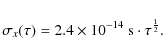
For our purposes, we express the above requirements for the MWL in a simplified form by the temporal Allan deviation
![]() expressed in
seconds, given by:
expressed in
seconds, given by:
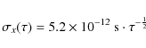
where the integration time
The temporal Allan deviation can be related to frequency instability in terms of the modified Allan deviation
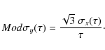
We assume that (1) and (2) represent our upper limits to the calculation of all perturbing effects in the following sections, together with the overall accuracy requirement (maximum allowed frequency bias) of
3 Relativistic model for clocks and time transfer of ACES
In a general relativistic framework, each clock produces its own local proper time, in our case
![]() and
and
![]() for ground and space clocks,
respectively.
for ground and space clocks,
respectively.
To model signal propagation between the ground and the space stations, we use a non-rotating geocentric space-time coordinate system. Thus, t=x0/cis the geocentric coordinate time, and
![]() are the spatial coordinates, where c is the speed of light in vacuum
(
c = 299 792 458 m s-1). We denote
are the spatial coordinates, where c is the speed of light in vacuum
(
c = 299 792 458 m s-1). We denote
![]() as the total Newtonian potential at the coordinate time t and the position
as the total Newtonian potential at the coordinate time t and the position
![]() with the convention that
with the convention that ![]() (Soffel et al. 2003). In these coordinates, the metric is given by an approximate solution of
Einstein's equations that is valid for low velocity and potential (
(Soffel et al. 2003). In these coordinates, the metric is given by an approximate solution of
Einstein's equations that is valid for low velocity and potential (
![]() and
and
![]() ):
):
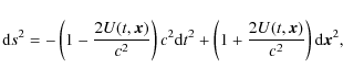 |
(4) |
where higher order terms can be neglected for our purposes (Wolf & Petit 1995).
In this system, each emission or reception event (at the antenna phase center) is identified by its coordinate time ti (Fig. 1) and a coordinate time interval is defined by
Tij=tj-ti. We define
![]() ,
,
![]() ,
and
,
and
![]() to be the position, velocity, and acceleration of the ground station, respectively, and
to be the position, velocity, and acceleration of the ground station, respectively, and
![]() ,
,
![]() ,
and
,
and
![]() to be the position, velocity, and acceleration of the space station,
respectively.
to be the position, velocity, and acceleration of the space station,
respectively.
| |
Figure 1: MWL principle. |
| Open with DEXTER | |
The ACES mission uses two different antennas: one Ku-band antenna for uplink and downlink, and one S-band antenna for downward signals only. The
antennae are characterized by their phase pattern, which describes the position of the antenna phase center as a function of the direction of the
incoming signal. The phase patterns of the MWL antennas have been measured in the laboratory at all three frequencies. For example, the phase
variations with direction of the Ku-band antenna can reach up to ![]() 0.1 rad (
0.1 rad (![]() 1 ps in time). Those variations can be corrected from the known
phase pattern and a knowledge of ISS attitude (i.e., direction of the incoming signal). Once corrected the remaining errors, mostly due to
uncertainties in ISS attitude, are below the MWL specifications.
1 ps in time). Those variations can be corrected from the known
phase pattern and a knowledge of ISS attitude (i.e., direction of the incoming signal). Once corrected the remaining errors, mostly due to
uncertainties in ISS attitude, are below the MWL specifications.
The f1 frequency signal is emitted by the ground station at the coordinate time t1 and received by the space station at t2. The f2 and f3 frequency signals are emitted from the space station at t3 and t5, and received at the ground station at t4 and t6. The third frequency is added to measure the TEC in the ionosphere, which allows the correction of the ionospheric delay.
The MWL is characterized by its continuous emission. It measures the time offsets between the locally generated and received signals. It provides three measurements (or observables) of the code (one on the space station, two on the ground) and three measurements of the phase of the carrier frequency at a sampling rate of one Hertz.
An observable is related to the phase comparison between a signal derived from the local oscillator and the received signal, corrected for the frequency difference mainly due to the first order Doppler effect (see Bahder 2003, for details of a similar procedure used in GPS). If we
consider a particular bit of the signal that is produced locally at
![]() and received at
and received at
![]() ,
an observable is a measurement of the local proper time interval between these two events. The true measurement of the phase difference
,
an observable is a measurement of the local proper time interval between these two events. The true measurement of the phase difference
![]() occurs at the single space-time point (
occurs at the single space-time point (
![]() ,
,
![]() )
and is labeled with the arrival proper time
)
and is labeled with the arrival proper time
![]() .
It can be expressed as
.
It can be expressed as
 |
(5) |
where
Considering the experimental uncertainties in the ACES mission (see Eqs. (1) and (2)), we neglect any terms in the relativistic model that, when maximised, lead to corrections of less than
![]() s in time. Numerical applications are necessary to evaluate which terms can be neglected. For this purpose, we consider the International Space Station with a circular trajectory at an altitude of 400 km in a plane inclined by
s in time. Numerical applications are necessary to evaluate which terms can be neglected. For this purpose, we consider the International Space Station with a circular trajectory at an altitude of 400 km in a plane inclined by
![]() with respect to the equatorial plane. Its velocity is
with respect to the equatorial plane. Its velocity is
![]() m s-1 in a gravitational potential of
m s-1 in a gravitational potential of
![]() .
The ground station has a velocity
.
The ground station has a velocity
![]() m s-1 at a gravitational potential of
m s-1 at a gravitational potential of
![]() .
.
The tropospheric delay
![]() is considered to be independent of the signal frequency, and slowly varying in time with an amplitude of less than 100 ns.
is considered to be independent of the signal frequency, and slowly varying in time with an amplitude of less than 100 ns.
We assume that the density of electrons in the ionosphere ![]() is lower than
is lower than
![]() electrons/m3. The ionospheric delay
electrons/m3. The ionospheric delay
![]() is maximum for the f3 frequency signal with an amplitude of less than 10 ns.
is maximum for the f3 frequency signal with an amplitude of less than 10 ns.
The relation between the proper time ![]() and the coordinate
time t is given to sufficient accuracy by
and the coordinate
time t is given to sufficient accuracy by
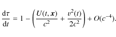
Higher order terms of Eq. (6) have negligible effects at the projected uncertainty of
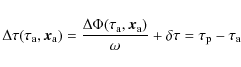
The ACES mission aims to measure the variation in the desynchronisation between ground and space clocks with time, that is to say, the function
![]() .
It is evaluated by combining the measurements performed on the ground and onboard the space station and a precise
calculation of the signal propagation times. To be able to control T23 (see below), we combine two measurements
.
It is evaluated by combining the measurements performed on the ground and onboard the space station and a precise
calculation of the signal propagation times. To be able to control T23 (see below), we combine two measurements
![]() and
and
![]() but with
but with
![]() .
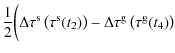
The expression of
desynchronisation then reads (see Duchayne 2008, for a detailed derivation)
.
The expression of
desynchronisation then reads (see Duchayne 2008, for a detailed derivation)
where
However, it is the derivative with respect to the coordinate time t of Eq. (7) that has to be studied for
applications such as the gravitational redshift test or geodesy, and then compared with the relation derived from Eq. (6):
We note that any constant term appearing in the desynchronisation given by Eq. (7) will have no effect on the final result in Eq. (8) because of the derivation.
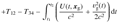
In (7), the difference
T12-T34 needs to be calculated from the knowledge of satellite and ground
positions and velocities (orbit determination). For example, T12 is the time interval elapsed between emission from the ground station and
reception by the satellite of the f1 frequency signal. It can be written as
where
Only one of the clocks (which we assume here to be the ground clock) has a known relation with coordinate time t, so
![]() cannot be directly obtained from the orbit determination, only
cannot be directly obtained from the orbit determination, only
![]() is known. Equation (9) is then modified to
is known. Equation (9) is then modified to
where
Assuming that
![]() s , the expression of
T12-T34, where all terms greater than
s , the expression of
T12-T34, where all terms greater than
![]() s have been included when
maximized for ACES can be evaluated by:
s have been included when
maximized for ACES can be evaluated by:
where
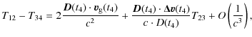
To obtain Eq. (11) we applied Eq. (10) to the upward and downward signals and expanded all positions and velocities in Taylor series around their values at t4, which can be obtained from the time of measurement (``label'' of the observable
![]() in Eq. (7)), on the ground.
in Eq. (7)), on the ground.
The difference T12 - T34 of upward and downward signals at f1 and f2 allows us to eliminate, to first order, delaying and restraining factors such as the range (D/c), and troposphere or Shapiro effects. Because of the asymmetry of the paths, that cancellation is not perfect, and some terms remain (Eq. (11)) that depend on orbit determination as well as on the coordinate time interval T23 elapsed between reception and emission at the phase center of the MWL antenna onboard the ISS.
The time interval T23 can be controlled by ``shifting'' the time of the measurements on the ground or onboard the space station (e.g., shifting
![]() in
in
![]() of Eq. (7)) when post-processing the data. This allows the control
of the difference between emission and reception at the clock. However, T23 given in Eq. (11) is defined at the antenna phase center, and therefore its control requires the knowledge (calibration and in situ measurement) of the instrumental delays (e.g., cables
and electronics) in the MWL space segment. So the control and knowledge (uncertainty
of Eq. (7)) when post-processing the data. This allows the control
of the difference between emission and reception at the clock. However, T23 given in Eq. (11) is defined at the antenna phase center, and therefore its control requires the knowledge (calibration and in situ measurement) of the instrumental delays (e.g., cables
and electronics) in the MWL space segment. So the control and knowledge (uncertainty
![]() )
of T23 is determined by the uncertainty in the calibration and measurement of internal delays, which also play a role in the following.
)
of T23 is determined by the uncertainty in the calibration and measurement of internal delays, which also play a role in the following.
The ionospheric effect
![]() on a radio signal of frequency f can be modelled by (Bassiri & Hajj 1993):
on a radio signal of frequency f can be modelled by (Bassiri & Hajj 1993):
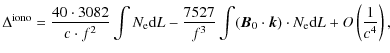
where
The electron density integrated along the signal trajectory,
![]() ,
is usually referred to as the total electron content (TEC). The
difference in the ionospheric delays in Eq. (11) is then
,
is usually referred to as the total electron content (TEC). The
difference in the ionospheric delays in Eq. (11) is then
The second and third term in Eq. (13) represent the effect of the Earth's magnetic field and reach at most 0.5 ps for ACES, which is almost negligible. Therefore, an approximate estimation of these terms is sufficient.
The TEC is determined by combining the two downward signal observables. The time interval T46 between the reception of the two signals depends
on the difference in their internal delays at the emission from the space station (i.e., T35) and the difference in their propagation time.
Assuming that
![]() s, the expression of the Total Electron Content is then given by:
s, the expression of the Total Electron Content is then given by:
where the final term in Eq. (14) is negligible when used for the time transfer (when inserted into Eq. (13)) but may be significant for the study of the TEC itself.
In summary, a reliable orbit determination is required for two main reasons: to calculate precisely the corrections in Eq. (11); and to evaluate correctly the terms on the right-hand side of Eq. (8) i.e., the second order Doppler and gravitational redshifts.
We also require a precise knowledge of the time interval T23, (i.e., of the onboard internal delays) to be able to calculate the corresponding terms in Eq. (11) with sufficient accuracy.
In this work, we aim to estimate using simple orbit error models, which levels of uncertainty in orbit determination and calibration of internal delays (knowledge of T23) are required to reach the required performances. For that purpose only the leading terms in Eq. (11) are required i.e.,
which, together with Eq. (8) for the relativistic frequency shift, is sufficient to derive the maximum allowed uncertainties in orbit determination and calibration of internal delays in order to stay below the limits given by Eqs. (1) and (2).
4 Effects of orbit errors on clock comparison
We now use Eqs. (15) and (8) to express the effects of station trajectory and time calibration uncertainties on both the time transfer and the relativistic frequency shift. In this section we make no assumptions about the orbit determination errors, our results being completely general and valid up to the neglected terms as described below.
We use (
![]() ,
,
![]() )
and (
)
and (
![]() ,
,
![]() )
for the true and computed
trajectories of the antenna phase center, respectively, and (
)
for the true and computed
trajectories of the antenna phase center, respectively, and (
![]() ,
,
![]() )
and (
)
and (
![]() ,
,
![]() )
for the true and computed trajectories of the clock reference point, respectively. We also define
(
)
for the true and computed trajectories of the clock reference point, respectively. We also define
(
![]() ,
,
![]() )
the true trajectory and the true velocity of the center of mass of the ISS. These five
trajectories are expressed in the non-rotating geocentric frame (GCRS, Geocentric Celestial Reference System) (Soffel et al. 2003).
)
the true trajectory and the true velocity of the center of mass of the ISS. These five
trajectories are expressed in the non-rotating geocentric frame (GCRS, Geocentric Celestial Reference System) (Soffel et al. 2003).
On the one hand, the error in the time transfer is related to the uncertainties in
T12 - T34, and can be obtained from the simplified Eq.
(15). It is dependent on the ground and space station trajectory knowledge, and on both the value of T23 and its uncertainty
![]() .
As said before, a precise knowledge of the time interval T23 is related to the internal delay calibrations. The error in
T12 - T34 is
.
As said before, a precise knowledge of the time interval T23 is related to the internal delay calibrations. The error in
T12 - T34 is
In general, ground station uncertainties are below 10 cm. Thus, the uncertainty in the ground station position is negligible with respect to the ISS position errors and the knowledge of the vector
Equation (16) can then be written as:
We note that Eq. (17) depends the antenna phase center position error (
On the other hand, the clock relativistic correction along a trajectory is obtained from Eq. (8). It depends on the position and the velocity of the reference point, in this case the clock. We need to express the error in the reference point frequency - i.e., the frequency difference between the true clock position and the computed clock position - to compare its Modified Allan deviation with the specifications.
The gravitational potential can be evaluated on a given trajectory with sufficient precision (Wolf & Petit 1995) using gravity models (e.g., GRIM5 or EGM96). The error in the frequency shift at the clock position is given by


The frequency difference between the reference point position


The trajectory of
where
Using
| (21) |
and to first order
 |
(22) |
and multiplying Eq. (20) by the vector
| = | |||
| = |  |
(23) |
We then obtain
which can be simplified to
 |
= |  |
|
 |
(25) |
In this expression the term
 can be
interpreted as the relativistic correction for the clock referenced to the local ISS frame. For an observer in the ISS frame, the non-gravitational
acceleration
can be
interpreted as the relativistic correction for the clock referenced to the local ISS frame. For an observer in the ISS frame, the non-gravitational
acceleration
Combining the previous equation with the same expressed in ![]() ,
we obtain
,
we obtain

In order to simplify Eq. (26), we evaluate the order of magnitude of the different contributors appearing in this equation.
To investigate the importance of the non-gravitational term
 ,
the drag was modeled
along a reference orbit of the ISS. A period with important solar activity was chosen to evaluate the worst case (see Fig. 2).
,
the drag was modeled
along a reference orbit of the ISS. A period with important solar activity was chosen to evaluate the worst case (see Fig. 2).
![\begin{figure}
\par\includegraphics[height=5.9cm]{09613fg2.eps} \end{figure}](/articles/aa/full_html/2009/35/aa09613-08/img166.png) |
Figure 2: Estimation of the non-gravitational acceleration of the ISS vs. time (in days) |
| Open with DEXTER | |
To estimate its effect on Eq. (26), the acceleration was multiplied by a 10 m bias, by a 10 meter random noise, or by a 10 m sinusoidal function at orbital period, corresponding to possible attitude and orbit error effects of the ISS. The Allan deviation remains below
10-21, which is totally negligible here. This term also has no effect on the frequency accuracy at the 10-16 level that ACES is designed to
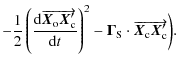
achieve. In addition, the residual term of the second order Doppler shift
![$\frac{1}{2 c^2} [(\frac{{\rm d} \overrightarrow{\vec{X}_{\rm o} \vec{X}_{\rm c}...
...(\frac{{\rm d}
\overrightarrow{\vec{X}_{\rm o} \vec{X}_{\rm c}'}}{{\rm d}t})^2]$](/articles/aa/full_html/2009/35/aa09613-08/img167.png) must be computed with the GCRS trajectories. The order of magnitude of these terms can be evaluated as
must be computed with the GCRS trajectories. The order of magnitude of these terms can be evaluated as
![]()
![]() with
with ![]() the orbital angular frequency,
the orbital angular frequency,
![]() ,
and
,
and ![]() its error. For
its error. For
![]() m and
m and
![]() m, this effect is also totally negligible.
m, this effect is also totally negligible.
The only important term in the performance evaluation is thus the along-track term
![]() ,
and Eq. (26) can be written
,
and Eq. (26) can be written
![$\displaystyle \frac{1}{c^{2}} \biggl[ \frac{{\rm d}} {{\rm d}
t}\left(\vec{V}_{\rm o}\cdot\overrightarrow{\vec{X}_{\rm c} \vec{X}_{\rm c}'} \right) \biggr].$](/articles/aa/full_html/2009/35/aa09613-08/img175.png)
Therefore, only the component of the clock position error
The scalar products of vectors can be evaluated in a local frame. For example, it may be useful to study them in the local orbital frame
(![]() ,
,
![]() ,
,
![]() )
defined by
)
defined by ![]() ,
which is the unit vector between the Earth's
center and the space station,
,
which is the unit vector between the Earth's
center and the space station, ![]() ,
which is orthogonal to
,
which is orthogonal to ![]() and the inertial velocity, and
and the inertial velocity, and ![]() ,
which is orthogonal to
,
which is orthogonal to ![]() and
and ![]() .
.
The ISS attitude is assumed to be roughly constant. The clock position error in this frame is represented by a constant vector (error in the position of the clock relative to the centre of mass), and by perturbations which produce
- attitude uncertainties (rigid body behaviour of ISS). If we take
 5 degrees uncertainty and a distance of 10 meters, this leads to a 0.87 m amplitude error in the clock position;
- ISS deformations: these are caused by thermoelastic effects, which will occur mainly at orbital period (eclipses and sun orientation). We suppose that these effects have an amplitude of below one meter;
- vibrations: here we assume that the ``vibrations'' are related to frequencies higher or equal to the first ISS eigenfrequency, which is higher than the orbital period. The corresponding displacements remain small and are expected to remain below one meter.
In summary, the errors in the time transfer and in the relativistic correction have been expressed as functions of the trajectory knowledge by means of Eqs. (17) and (27). Only the error in the knowledge of the ISS center of mass position plays a significant role in the relativistic correction.
5 Orbit error examples
We now describe two simple models for ISS orbit errors as examples of investigating numerically the effect that they should have on ACES performance.
We consider two methods used to evaluate the orbit of a satellite. On the one hand, the dynamical method takes into account the equations of motion to estimate the trajectory, it fits the measured data with an orbit satisfying the principles of celestial mechanics, and estimates a number of parameters that provide the best fit trajectory. On the other hand, the kinematical method uses the measurements of the satellite position (e.g., GPS data) directly with no a priori assumption about the form of the orbit. In both cases, the resulting orbit errors are in general not easily described by a simple model, but for our purposes we use two examples that should approximately reflect the orders of magnitude of the main orbit error contributions.
For dynamical orbit determination, the differences between the true and computed trajectories of the ISS center of mass are expected to show specific structures. For example, an eccentricity error has no long-term effect, but periodic errors can be important, and the radial, along track, and velocity errors are all correlated. For weak eccentricity orbits, the difference between two real orbits is given by the Hill model (or the Clohessy-Wiltshire model), which is an expansion of the uncertainties relative to a reference circular orbit (Colombo 1986; Colombo et al. 2004). If we suppose that a set of parameters exists that perfectly describes the true orbit of the ISS, then this model is a first approximation to the errors in the center of mass between the computed and the true orbits.
For kinematical orbit determination, one expects little a priori correlation between the different orbital error components. We therefore use a simple independent random noise on each component as a first approximation.
In the Hill model, the position uncertainties along the radial, tangential, and normal axis (in the local ISS frame) are given as follows:
where X, Y, cR, and dR are amplitude coefficients, and where
6 Numerical results
We now use the previously described error models to calculate the corresponding constraints imposed by the ACES stability (Eqs. (1) and (2)) and accuracy requirements, by means of Eqs. (17) and (27). We first consider the Hill model, followed by results for a simple random noise.
We consider orbit error models in the local (![]() ,
,
![]() ,
,
![]() )
frame, so we need to transform them to the GCRS and determine the uncertainties in this frame in position and velocity parameters. We consider an ephemeris of the ISS corresponding to the 20th of May, 2005 and a ground station based in Toulouse, France
)
frame, so we need to transform them to the GCRS and determine the uncertainties in this frame in position and velocity parameters. We consider an ephemeris of the ISS corresponding to the 20th of May, 2005 and a ground station based in Toulouse, France
![]() .
This station has indeed been chosen as the master ground station of the ACES mission. All station parameters and their uncertainties have to be expressed in the same frame (i.e., GCRS).
.
This station has indeed been chosen as the master ground station of the ACES mission. All station parameters and their uncertainties have to be expressed in the same frame (i.e., GCRS).
We first consider the error in the time transfer given by Eq. (17). We choose the signs of the independent parameters
(
![]() ,
T23, and
,
T23, and
![]() )
so as to maximize the resulting temporal Allan deviation. The calculated deviation must
be compared with the MWL specifications.
)
so as to maximize the resulting temporal Allan deviation. The calculated deviation must
be compared with the MWL specifications.
Assuming that the error in T23 is negligible (i.e.,
![]() s), for all values of the factor X (or Y) in Eq.
(28), it is possible to determine the maximum value of the time interval T23 for which the temporal Allan deviation remains
smaller than the specifications. For numerous values of X, we calculate a bound that delineates two different areas: the allowed uncertainties
area in which each couple of parameters (X, T23) gives a deviation staying under the specifications, and the prohibited area.
s), for all values of the factor X (or Y) in Eq.
(28), it is possible to determine the maximum value of the time interval T23 for which the temporal Allan deviation remains
smaller than the specifications. For numerous values of X, we calculate a bound that delineates two different areas: the allowed uncertainties
area in which each couple of parameters (X, T23) gives a deviation staying under the specifications, and the prohibited area.
![\begin{figure}
\par\includegraphics[width=8.5cm]{09613fg3.eps}
\end{figure}](/articles/aa/full_html/2009/35/aa09613-08/img189.png) |
Figure 3:
The maximum allowed value of T23 as a function of the scale factor X to comply with the specifications, assuming
|
| Open with DEXTER | |
Figure 3 shows that, the shorter the time interval T23, the larger the allowed uncertainty in the space station position.
This result provides a way to combine upwards and downwards signals to allow the maximum uncertainty in space station position and to comply with the
specifications. The most favorable situation is when the reception at the antenna phase center of the space station corresponds to the emission at
the same place i.e., t2 = t3 (see Fig. 4). This way of combining signals is named the ``![]() configuration''. To
work with parameters in the asymptotic area (see Fig. 3) we require T23 to be below 10-6 s.
configuration''. To
work with parameters in the asymptotic area (see Fig. 3) we require T23 to be below 10-6 s.
| |
Figure 4:
The `` |
| Open with DEXTER | |
If we then plot the maximum value of
![]() for all values of the factor X, there will be two asymptotic values that we cannot cross if we
want to stay within the specifications (see Fig. 5). Basically a compromise between the knowledge of the space
station trajectory and the precision of the internal delay calibration must be achieved owing to the maximization of the Allan deviation. We will
evaluate the maximum allowed errors in these two parameters if no other errors are present.
for all values of the factor X, there will be two asymptotic values that we cannot cross if we
want to stay within the specifications (see Fig. 5). Basically a compromise between the knowledge of the space
station trajectory and the precision of the internal delay calibration must be achieved owing to the maximization of the Allan deviation. We will
evaluate the maximum allowed errors in these two parameters if no other errors are present.
![\begin{figure}
\par\includegraphics[height=5cm]{09613fg5.eps}
\end{figure}](/articles/aa/full_html/2009/35/aa09613-08/img191.png) |
Figure 5:
Maximum allowed value of
|
| Open with DEXTER | |
We search for the asymptotic value of factors X and Y that comply with the specifications for all phases (![]() ,
,
![]() )
when we have
no error in T23. The asymptotic value for the orbit determination is obtained for X, Y = 4200 m, which corresponds to a 4.2 km error in the
tangential and normal axes, and to a 2.1 km error in the radial axis.
)
when we have
no error in T23. The asymptotic value for the orbit determination is obtained for X, Y = 4200 m, which corresponds to a 4.2 km error in the
tangential and normal axes, and to a 2.1 km error in the radial axis.
The asymptotic value of the time calibration does not depend on the orbit determination uncertainties. So it is independent of the phases ![]() and
and ![]() .
We can then draw the temporal Allan deviations for different values of
.
We can then draw the temporal Allan deviations for different values of
![]() (see Fig.
6). We find that
(see Fig.
6). We find that
![]() must stay below à
must stay below à
![]() s.
s.
![\begin{figure}
\par\includegraphics[width=9cm]{09613fg6.eps}
\end{figure}](/articles/aa/full_html/2009/35/aa09613-08/img195.png) |
Figure 6:
Temporal Allan deviations for X = 0, T23= 0 s and
|
| Open with DEXTER | |
The requirements for several passes have also been investigated. In this case, the calculated deviations have to be compared to the specifications given by Eq. (2). The results have shown that the requirements on orbit determination and time calibration are less stringent for several passes than for a single pass. Therefore, if specifications are respected for a single pass, specifications for longer integration times are also respected.
We now evaluate the requirements on orbit determination considering the relativistic frequency shift. We search for the maximum value of X to
comply with the specifications given by Eqs. (1) and (2). Equation (27) is evaluated
with the error model in Eq. (28), and its Allan deviation is calculated for different values of X. For integration times longer
than one thousand seconds, these Allan deviations are independent of the phases ![]() and
and ![]() .
.
![\begin{figure}
\par\includegraphics[height=5.3cm]{09613fg7.eps}
\end{figure}](/articles/aa/full_html/2009/35/aa09613-08/img196.png) |
Figure 7: Modified Allan deviations of the redshift error for X=14, 16, 18, 20 m. |
| Open with DEXTER | |
Figure 7 shows that, if the factor X in Eq. (28) equals 16 m i.e., if we have an eight meter error in the radial position and a sixteen meter error in the tangential position, then we comply with the specifications.
Because of the projection of the position error along the ISS center of mass velocity (see Eq. (27)), the requirement on the factor Y is orders of magnitude less stringent. The bound is determined by the asymptotic value arising from the time transfer (see Eq. (17) and Fig. 5).
We now turn to the second example of orbit determination errors: independent random errors in ![]() ,
,
![]() ,
and
,
and
![]() .
We consider white noise of amplitude (standard deviation)
.
We consider white noise of amplitude (standard deviation) ![]() ,
,
![]() ,
and
,
and ![]() at one second sampling
intervals for each of the three components.
at one second sampling
intervals for each of the three components.
As for the Hill model, the by far more stringent constraints come from the effect of these errors in the relativistic frequency shift given by Eq.
(27). In particular, a white noise ![]() in Eq. (27) will translate into a temporal Allan variance given by
in Eq. (27) will translate into a temporal Allan variance given by
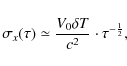
which satisfies the requirements Eqs. (1) and (2) for all integration times when
Because of the projection of the error onto
![]() in Eq. (27), the relativistic frequency shift imposes virtually
no limits on the normal and radial components of the errors. These are limited by the effect on the time transfer given by Eq.
(17). Assuming that
in Eq. (27), the relativistic frequency shift imposes virtually
no limits on the normal and radial components of the errors. These are limited by the effect on the time transfer given by Eq.
(17). Assuming that
![]() s and
s and
![]() s (see above), the first term of that
equation is by far dominant. Maximizing the dot product in that term, we obtain an upper limit of 1.4 km to both
s (see above), the first term of that
equation is by far dominant. Maximizing the dot product in that term, we obtain an upper limit of 1.4 km to both ![]() and
and ![]() when
remaining within specifications for all integration times.
when
remaining within specifications for all integration times.
Finally, we consider the accuracy requirement of ACES, i.e., 10-16 in relative frequency when averaged over ten days. From the integral of Eq.
(27), this implies that the tangential component of the position error
(
![]() )
in Eq. (27))
cumulated over ten days needs to remain below one kilometer (including for example the linear term along the tangential axis in Eq.
(28)). This is unlikely to raise any difficulty, if the far more stringent requirements from periodic or random errors (see above)
are met. We note that the accuracy requirement is related to a requirement on the knowledge and conservation of the total energy of the orbit. An
error in the total energy will show up as a velocity bias, and thus as a linear term along the tangential axis. The non-conservation of the total
energy (non-gravitational accelerations) was found to be negligible in Sect. 4. Nonetheless, possible long-term effects, if they exist,
will lead to a slow variation in the tangential error. The constraint on both the error in the total energy and the effects due to energy
non-conservation is provided by the accuracy requirement, i.e., that the tangential error cumulated over ten days needs to remain below one
kilometer.
)
in Eq. (27))
cumulated over ten days needs to remain below one kilometer (including for example the linear term along the tangential axis in Eq.
(28)). This is unlikely to raise any difficulty, if the far more stringent requirements from periodic or random errors (see above)
are met. We note that the accuracy requirement is related to a requirement on the knowledge and conservation of the total energy of the orbit. An
error in the total energy will show up as a velocity bias, and thus as a linear term along the tangential axis. The non-conservation of the total
energy (non-gravitational accelerations) was found to be negligible in Sect. 4. Nonetheless, possible long-term effects, if they exist,
will lead to a slow variation in the tangential error. The constraint on both the error in the total energy and the effects due to energy
non-conservation is provided by the accuracy requirement, i.e., that the tangential error cumulated over ten days needs to remain below one
kilometer.
7 Conclusion
We have derived detailed and general (within the specified assumptions) expressions for the calculation of the effect of orbit determination and instrumental calibration errors, on the stability and accuracy of ground to space clock comparisons. These expressions were then used for the specific example of the ACES mission to derive the maximum allowed errors given the stability requirements of that mission. For that purpose, we used two simplified orbit error models (Hill model and random noise), setting limits on the appropriate parameters of those models. Although neither of those models is likely to reflect all of the ISS orbit errors correctly, they are nonetheless expected to provide reliable order of magnitude estimates of the maximum allowed orbit determination uncertainties. These are summarized in Table 1, where in each column we have provide the more stringent result of the two models.
Table 1: Requirements on orbit determination and internal delay calibration.
Furthermore, we have identified an optimal way of combining upward and downward signals (the ![]() configuration), which allows for the maximum
orbit determination errors. This then provides a constraint on the maximum allowed value of
configuration), which allows for the maximum
orbit determination errors. This then provides a constraint on the maximum allowed value of
![]() s and its maximum allowed
uncertainty of
s and its maximum allowed
uncertainty of
![]() s,
which constrains the required knowledge of the sum (transmission + reception) of instrumental delays
between the antenna phase centre and the onboard clock (also provided in Table 1).
s,
which constrains the required knowledge of the sum (transmission + reception) of instrumental delays
between the antenna phase centre and the onboard clock (also provided in Table 1).
Finally, the accuracy requirement of ACES was used to constrain long-term (![]() 10 days) linear drifts and other slow variations in the orbit
determination errors. We find that the total tangential error cumulated over 10 days needs to remain below
1 km to comply with the accuracy
specification (10-16 in relative frequency after ten days of averaging), which should pose no particular problems given the more stringent
short-term requirements (see Table 1).
10 days) linear drifts and other slow variations in the orbit
determination errors. We find that the total tangential error cumulated over 10 days needs to remain below
1 km to comply with the accuracy
specification (10-16 in relative frequency after ten days of averaging), which should pose no particular problems given the more stringent
short-term requirements (see Table 1).
In conclusion, the requirements on the orbit determination are significantly less stringent than the initial 'naive' estimate (one meter error for 10-16 in relative frequency), which is mainly due to partial cancelation between the gravitational redshift and the second order Doppler effect in the relativistic frequency correction of the onboard clock.
Acknowledgements
The research project is supported by the French space agency CNES and ESA through Loïc Duchayne's research scholarship No. 05/0812.
References
- Allan, D. W., & Ashby, N. 1986, in Relativity in Celestial Mechanics and Astronomy, ed. J., Kovalevsky, & V. A., Brumberg, Proc. IAU Symp., 114, Leningrad 1985 (Dordrecht: Reidel Publ.) (In the text)
- Bahder, T. B. 2003, Phys. Rev. D, 68, 063005 [NASA ADS] [CrossRef] (In the text)
- Bassiri, S. & Hajj, G. A. 1993, ISSN 0065-3438, 1071 (In the text)
- Bize, S., Laurent, P., Abgrall, M., et al. 2005, J. Phys. B: At. Mol. Opt. Phys., 38, S449 [NASA ADS] [CrossRef] (In the text)
- Bjerhammar, A. 1985, Bull. Geod., 59, 207 [CrossRef] (In the text)
- Blanchet, L., Salomon, C., Teyssandier, P., Wolf, P., et al. 2001, A&A, 370, 320 [NASA ADS] [CrossRef] [EDP Sciences] (In the text)
- Colombo, O. L. 1986, Bulletin géodésique, 60, 64 [NASA ADS] [CrossRef] (In the text)
- Colombo, O. L., et al. 2004, Proceedings of the Institute Of Navigation GNSS Meeting (In the text)
- Duchayne, L. 2008, Ph.D. dissertation, in French, available on http://tel.archives-ouvertes.fr/index.php (In the text)
- Heavner, T. P., Jefferts, S. R., Donley, E. A., Shirley, J. H., Parker, T. E., et al. 2005, Metrologia, 42, 411 [NASA ADS] [CrossRef] (In the text)
- Klioner, S. A. 1992, Celest. Mech. Dynam. Astron., 53, 81 [NASA ADS] [CrossRef] (In the text)
- Linet, B., & Teyssandier, P. 2002, Phys. Rev. D, 66, 024045 [NASA ADS] [CrossRef] (In the text)
- Oskay, W. H., et al. 2006, Phys. Rev. Lett., 97, 020845 [CrossRef] (In the text)
- Petit, G., & Wolf, P. 1994, A&A, 286, 971 [NASA ADS] (In the text)
- Rosenband, T., Hume, D. B., Schmidt, P. O., et al. 2008, Science, 319, 1808 [NASA ADS] [CrossRef] (In the text)
- Shapiro, I. I. 1964, Phys. Rev. Lett., 13, 789 [NASA ADS] [CrossRef] (In the text)
- Soffel, M. 2003, AJ, 126, 2687 [NASA ADS] [CrossRef] (In the text)
- Soffel, M., Rakuljic, G. A., Yariv, A., et al. 1988, Manuscripta Geodetica, 13 143 (In the text)
- Wolf, P., & Petit, G. 1995 A&A, 304, 653 (In the text)
All Tables
Table 1: Requirements on orbit determination and internal delay calibration.
All Figures
| |
Figure 1: MWL principle. |
| Open with DEXTER | |
| In the text | |
| |
Figure 2: Estimation of the non-gravitational acceleration of the ISS vs. time (in days) |
| Open with DEXTER | |
| In the text | |
| |
Figure 3:
The maximum allowed value of T23 as a function of the scale factor X to comply with the specifications, assuming
|
| Open with DEXTER | |
| In the text | |
| |
Figure 4:
The `` |
| Open with DEXTER | |
| In the text | |
| |
Figure 5:
Maximum allowed value of
|
| Open with DEXTER | |
| In the text | |
| |
Figure 6:
Temporal Allan deviations for X = 0, T23= 0 s and
|
| Open with DEXTER | |
| In the text | |
| |
Figure 7: Modified Allan deviations of the redshift error for X=14, 16, 18, 20 m. |
| Open with DEXTER | |
| In the text | |
Copyright ESO 2009
Current usage metrics show cumulative count of Article Views (full-text article views including HTML views, PDF and ePub downloads, according to the available data) and Abstracts Views on Vision4Press platform.
Data correspond to usage on the plateform after 2015. The current usage metrics is available 48-96 hours after online publication and is updated daily on week days.
Initial download of the metrics may take a while.