| Issue |
A&A
Volume 504, Number 1, September II 2009
|
|
|---|---|---|
| Page(s) | 259 - 276 | |
| Section | Planets and planetary systems | |
| DOI | https://doi.org/10.1051/0004-6361/200911760 | |
| Published online | 15 July 2009 | |
A grid of polarization models for Rayleigh scattering planetary atmospheres![[*]](/icons/foot_motif.png)
E. Buenzli - H. M. Schmid
Institute for Astronomy, ETH Zurich, 8093 Zurich, Switzerland
Received 30 January 2009 / Accepted 27 June 2009
Abstract
Context. Reflected light from giant planets is polarized by scattering, offering the possibility of investigating atmospheric properties with polarimetry. Polarimetric measurements are available for the atmospheres of solar system planets, and instruments are being developed to detect and study the polarimetric properties of extrasolar planets.
Aims. We investigate the intensity and polarization of reflected light from planets in a systematic way with a grid of model calculations. Comparison of the results with existing and future observations can be used to constrain parameters of planetary atmospheres.
Methods. We present Monte Carlo simulations for planets with Rayleigh scattering atmospheres. We discuss the disk-integrated polarization for phase angles typical of extrasolar planet observations and for the limb polarization effect observable for solar system objects near opposition. The main parameters investigated are single scattering albedo, optical depth of the scattering layer, and albedo of an underlying Lambert surface for a homogeneous Rayleigh scattering atmosphere. We also investigate atmospheres with isotropic scattering and forward scattering aerosol particles, as well as models with two scattering layers.
Results. The reflected intensity and polarization depend strongly on the phase angle, as well as on atmospheric properties, such as the presence of absorbers or aerosol particles, column density of Rayleigh scattering particles and cloud albedo. Most likely to be detected are planets that produce a strong polarization flux signal because of an optically thick Rayleigh scattering layer. Limb polarization depends on absorption in a different way than the polarization at large phase angles. It is especially sensitive to a vertical stratification of absorbers. From limb polarization measurements, one can set constraints on the polarization at large phase angles.
Conclusions. The model grid provides a tool for extracting quantitative results from polarimetric measurements of planetary atmospheres, in particular on the scattering properties and stratification of particles in the highest atmosphere layers. Spectropolarimetry of solar system planets offers complementary information to spectroscopy and polarization flux colors can be used for a first characterization of exoplanet atmospheres.
Key words: polarization - scattering - techniques: polarimetric - planetary systems - planets and satellites: general
1 Introduction
Light reflected from planetary atmospheres is generally polarized. The reflection is the result of different types of scattering particles with characteristic polarization properties. Polarimetric observations therefore provide information on the atmospheric structure and on the nature of scattering particles that complements other observations. Systematic model calculations are required to interpret the available polarimetry from solar system planets and prepare for future polarimetric measurements of extrasolar planets.
Scattering processes.
Rayleigh scattering occurs on particles much smaller than the
wavelength of the scattered light. This process produces 100%
polarization for a single right angle scattering.
Rayleigh scattering is much stronger for short wavelengths because
the cross section behaves like
![]() ,
and it
favors forward and backward scattering, which are both equally strong.
The blue sky in Earth's atmosphere is a well known example of
Rayleigh scattering by molecules.
,
and it
favors forward and backward scattering, which are both equally strong.
The blue sky in Earth's atmosphere is a well known example of
Rayleigh scattering by molecules.
Aerosol haze particles with a size roughly comparable to the
wavelength can produce strongly forward directed
scatterings. Depending on the structure of the particle, a high
(p>90%) or low (
![]() %)
fractional polarization results for a scattering angle of
%)
fractional polarization results for a scattering angle of ![]() .
For example, the maximum polarization
for scattering by optically thin zodiacal or cometary dust is not more
than
.
For example, the maximum polarization
for scattering by optically thin zodiacal or cometary dust is not more
than
![]() % (e.g. Leinert et al. 1981; Levasseur-Regourd et al. 1996), while a polarization close to 100% is inferred for single scattering of haze
particles in Saturn's moon Titan (Tomasko et al. 2008).
% (e.g. Leinert et al. 1981; Levasseur-Regourd et al. 1996), while a polarization close to 100% is inferred for single scattering of haze
particles in Saturn's moon Titan (Tomasko et al. 2008).
Liquid droplets in clouds produce a polarization because of
refraction and reflection, which can be particularly high (>50%) for scattering angles of about ![]() for spherical water droplets,
corresponding to the primary rainbow (see e.g. Bailey
2007). Clouds made of ice crystals reflect and refract light
in many different ways, and no distinct polarization features like rainbows are
expected, except locally, where ice crystals may have very similar structures.
for spherical water droplets,
corresponding to the primary rainbow (see e.g. Bailey
2007). Clouds made of ice crystals reflect and refract light
in many different ways, and no distinct polarization features like rainbows are
expected, except locally, where ice crystals may have very similar structures.
Multiple scatterings in planetary atmospheres randomize the polarization direction of the single scatterings and lower the observable polarization significantly. Therefore the net polarization of the reflected light depends not only on the scattering angle and the properties of the scattering particles, but also on the atmospheric structure. For this reason it is not suprising that a large diversity of polarization properties exists for the solar system planets.
Observations.
Venus shows a low (<5%) negative polarization, which is a polarization parallel to the scattering plane, for most phase angles . In the blue and UV, a rainbow feature with a positive polarization of several percent is present (e.g. Coffeen & Gehrels 1969; Dollfus & Coffeen 1970), indicating that the reflection occurs mainly from droplets in optically thick clouds (Hansen & Hovenier 1974).
For the giant planets, only observations near opposition are possible with earth-bound observations. Near opposition the disk-integrated polarization is low because single back-scattering is unpolarized and multiple scattering polarization cancels for a symmetric planet.
With disk-resolved observations of Jupiter, Lyot (1929) first detected that the Jovian poles show a strong limb polarization of order 5-10%. To understand this effect one has to consider a back-scattering situation at the limb of a sphere, where locally we have a configuration of grazing incidence and grazing emergence (for a plane parallel atmosphere) for the incoming and the back-scattered photons, respectively. Photons scattered upwards will mostly escape without a second scattering, and photons scattered down have a low probability of being reflected towards us after the second scattering, but a high probability of being absorbed or undergoing multiple scatterings. Thus photons that are reflected towards us by two scatterings travel predominantely parallel to the surface. Because the polarization angle induced in a single dipole-type scattering process, like Rayleigh scattering, is perpendicular to the propagation direction of the incoming photon, a polarization perpendicular to the limb is produced.
Measurements at large phase angles
![]() for Jupiter with
spacecrafts detected a polarization of
for Jupiter with
spacecrafts detected a polarization of
![]() % for the poles while the
polarization is much lower (<10%) for the equatorial region
(Smith & Tomasko 1984).
The high polarization at the poles can be explained by reflection from
a scattering aerosol haze layer, while the polarization at the equator is low
because of reflection from clouds. Towards short wavelengths (blue) the
polarization at the equator increases strongly, indicating that also
Rayleigh scattering contributes to the resulting polarization.
% for the poles while the
polarization is much lower (<10%) for the equatorial region
(Smith & Tomasko 1984).
The high polarization at the poles can be explained by reflection from
a scattering aerosol haze layer, while the polarization at the equator is low
because of reflection from clouds. Towards short wavelengths (blue) the
polarization at the equator increases strongly, indicating that also
Rayleigh scattering contributes to the resulting polarization.
For Saturn the polarization is qualitatively similar to Jupiter with an enhanced polarization at the poles at short wavelengths (blue). In the red the polarization level of the poles is lower than for Jupiter (Tomasko & Doose 1984).
Uranus and Neptune display a strong limb polarization along the entire limb (Schmid et al. 2006a; Joos & Schmid 2007). Albedo spectra (e.g. Baines & Bergstralh 1986) and the polarization indicate that Rayleigh scattering is predominant in these atmospheres.
An interesting case is Saturn's moon Titan, which has a thick
scattering layer of photochemical haze that produces a very
high disk-integrated polarization of ![]() % in the B and
R band (Tomasko & Smith 1982). More recently the Huygens
probe measured the scattering and polarization properties of the aerosol
particles in great detail during its descent through Titan's
atmosphere (Tomasko et al. 2008).
% in the B and
R band (Tomasko & Smith 1982). More recently the Huygens
probe measured the scattering and polarization properties of the aerosol
particles in great detail during its descent through Titan's
atmosphere (Tomasko et al. 2008).
The observations show that Rayleigh scattering is
an important polarigeneric process in atmospheres of solar system
objects, in particular for Uranus and Neptune, and for the equatorial regions of
Jupiter and Saturn. Besides Rayleigh scattering one has to consider the reflection from
haze particles (aerosols). Scattering by small aerosol particles
![]() may be approximated by Rayleigh scattering. For
large particles,
may be approximated by Rayleigh scattering. For
large particles,
![]() ,
the strong forward scattering effect
and the reduced polarization for right angle scattering cause
significant differences when compared to Rayleigh scattering.
,
the strong forward scattering effect
and the reduced polarization for right angle scattering cause
significant differences when compared to Rayleigh scattering.
Clouds dominate in the atmosphere of Venus, and at longer wavelengths (red) also in Saturn and Jupiter. The reflection from clouds produces only a low positive or even negative polarization signal in Venus, Saturn or Jupiter, typically at a level p <5%. In a first approximation one may therefore treat clouds like a diffusely scattering layer producing no polarization.
Polarimetric measurements of stellar systems with known extrasolar planets were attempted, but up to now no convincing detection of the polarized reflected light from an extrasolar planet has been made (Lucas et al. 2009; Wiktorowicz 2009). The deduced upper limits on the polarization flux from the close-in planet indicate that these objects are not covered with a well reflecting Rayleigh scattering layer.
Model calculations.
The classical theory for the analytic solution of the multiple scattering problem is treated in the seminal work of Chandrasekhar (1950), from which the polarization of conservative (non-absorbing) Rayleigh scattering planets can be derived. Van de Hulst (1980) gives a comprehensive overview on theoretical work up to that time including many numerical model results.
Schmid et al. (2006a) put together available model results useful for parameter studies of the polarization from Rayleigh scattering atmospheres. This includes the following model results:
- phase curves for the disk-integrated intensity and polarization for finite, conservative (no absorption) Rayleigh scattering atmospheres for different optical thicknesses and ground albedos from Kattawar & Adams (1971);
- the limb polarization at opposition for semi-infinite Rayleigh scattering atmospheres with different single scattering albedos derived from formulas and tabulated functions given in Abhyankar & Fymat (1970, 1971) and Chandrasekhar (1950);
- the limb polarization at opposition for finite, conservative (no absorption) Rayleigh scattering atmospheres for different optical thicknesses and ground albedos from tabulations given in Coulson et al. (1960).
Another line of investigation now concentrates on the expected polarization of extrasolar planets. The Rayleigh and Mie scattering polarization of close-in planets was investigated by Seager et al. (2000). These calculations consider planets which are unresolved from their central star and the polarization signal is strongly diluted by the unpolarized stellar light.
Stam et al. (2004) modeled the polarization of a Jupiter-like extrasolar planet with methane absorption bands for three special cases and presented polarization spectra and wavelength integrated phase curves. Also monochromatic phase curves for a non-absorbing clear and a hazy atmosphere are available (Stam et al. 2006). Other studies determined the expected polarization from clouds of terrestrial planets (e.g. Bailey 2007) or the polarization of extrasolar analogs to Earth (Stam 2008).
Despite all these models systematic model calculations are sparse in the literature. For finite Rayleigh scattering atmospheres, polarization phase curves have been calculated only for few selected cases. No results are available for the limb polarization of atmospheres with finite thickness and absorption.
It is the goal of this paper to present a grid of model results for Rayleigh scattering models with absorption and to explore the model parameter space in a systematic way. The results should allow a comparison with observations and provide a tool for their interpretation. Additionally effects of selected deviations from simple Rayleigh scattering models will be discussed.
In the next section the paper describes our scattering model and the
Monte Carlo simulations. Section 3 presents the results from a
comprehensive Rayleigh scattering model grid covering the three atmosphere
parameters: single scattering albedo ![]() ,
optical thickness of the Rayleigh
scattering layer
,
optical thickness of the Rayleigh
scattering layer
![]() ,
and albedo of the underlying reflecting
surface
,
and albedo of the underlying reflecting
surface ![]() .
In Sect. 4 we explore the effects of a mixure of isotropic and Rayleigh scattering, of particles with a forward scattering phase function, and of two polarizing layers. In Sect. 5 we discuss spectral dependences. Section 6 highlights some special cases and diagnostic diagrams which may be of particular interest for the interpretation of
observational data. A discussion and conclusions are given in the final
section. Appendix A describes the tables with the numerical results of our calculations of intensity and polarization phase curves for a grid of 333 model parameter combinations. These are available in electronic form at the CDS.
.
In Sect. 4 we explore the effects of a mixure of isotropic and Rayleigh scattering, of particles with a forward scattering phase function, and of two polarizing layers. In Sect. 5 we discuss spectral dependences. Section 6 highlights some special cases and diagnostic diagrams which may be of particular interest for the interpretation of
observational data. A discussion and conclusions are given in the final
section. Appendix A describes the tables with the numerical results of our calculations of intensity and polarization phase curves for a grid of 333 model parameter combinations. These are available in electronic form at the CDS.
2 Model description
Our planet model consists of a spherical body of radius R, illuminated
by a parallel beam. This geometry is appropriate for not rapidely rotating
planets with a large separation, ![]() ,
from the parent star.
Each surface element is approximated by a plane parallel atmosphere. This
simplification is reasonable for planets
without an extended, tenuous atmosphere.
,
from the parent star.
Each surface element is approximated by a plane parallel atmosphere. This
simplification is reasonable for planets
without an extended, tenuous atmosphere.
2.1 Intensity and polarization parameters
The intensity and polarization of the reflected light is described by the
Stokes vector
![]() .
The linear polarized
intensity or polarization flux is defined by the parameters
Q=I0-I90 and
U=I45-I135, where the indices
stand for the polarization direction with respect to a specified direction
in the selected coordinate system. In this paper only processes producing
linear polarization are studied and therefore the Stokes parameter V
for the circular polarization is omitted.
We express the fractional polarization by the symbols
.
The linear polarized
intensity or polarization flux is defined by the parameters
Q=I0-I90 and
U=I45-I135, where the indices
stand for the polarization direction with respect to a specified direction
in the selected coordinate system. In this paper only processes producing
linear polarization are studied and therefore the Stokes parameter V
for the circular polarization is omitted.
We express the fractional polarization by the symbols
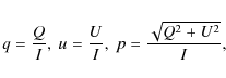 |
(1) |
and the polarized intensity
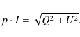 |
(2) |
For the study of the limb polarization in resolved solar system planets at opposition we introduce the radial Stokes parameter Qr, which is positive for an orientation of the polarization parallel to the radius vector
The radial polarization curves qr(r) and Qr(r) can only be observed if the planetary disk is well resolved. The measured radial profile depends strongly on the achieved spatial resolution. Because of the limited spatial resolution of most observations it is very hard to exactly measure the polarization near the limb. It is much less difficult to evaluate a disk-integrated polarization or polarization flux and to estimate and correct the degradation of the observed value with respect to the intrinsic value with a simulation of the observational resolution or point spread function. This approach is described in detail in Schmid et al. (2006a) for seeing limited polarimetry of Uranus and Neptune.
Therefore we mainly discuss the intensity weighted
polarization
![]() ,
which is the equivalent to
the disk-integrated radial polarization
,
which is the equivalent to
the disk-integrated radial polarization
![]() normalized to the geometric albedo.
The geometric albedo
normalized to the geometric albedo.
The geometric albedo
![]() is the disk-integrated reflected intensity
of a given model at opposition normalized to the reflection of a white Lambertian disk. It corresponds to
is the disk-integrated reflected intensity
of a given model at opposition normalized to the reflection of a white Lambertian disk. It corresponds to
![]() in our calculations.
in our calculations.
The radial polarization curves are qualitatively similar for most models. The
shape of the intensity curve varies significantly from limb darkening to limb brightening for different
model parameteres and cannot
solely be described by the geometric albedo. Additionally we choose the Minnaert law exponent k as fit parameter for the shape of the center-to-limb intensity curve.
The Minnaert law for opposition is
![]() ,
where
,
where
![]() .
This yields the following one-parameter fit curve
I(r) = Ir=0 (1-r2)k-1/2.
.
This yields the following one-parameter fit curve
I(r) = Ir=0 (1-r2)k-1/2.
2.2 Atmosphere parameters
The plane parallel atmosphere is assumed to consist of a homogeneous scattering layer that is either semi-infinite or finite with a reflecting (cloud or ground) Lambertian surface layer with a surface albedo. The basic model atmospheres are described by three parameters:
- the single scattering albedo
 ;
;
- the (vertical) optical thickness for scattering,
 ,
of the scattering layer;
,
of the scattering layer;
- the albedo
 of the surface below the scattering layer.
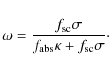 |
(3) |
The value
The optical depth for scattering
![]() follows from the column density Z of the scattering layer:
follows from the column density Z of the scattering layer:
![]() ,
where
,
where ![]() is the scattering cross section per particle.
The semi-infinite case corresponds to
is the scattering cross section per particle.
The semi-infinite case corresponds to
![]() .
We treat absorption like an addition of absorption optical depth to a
layer with a given scattering optical depth
.
We treat absorption like an addition of absorption optical depth to a
layer with a given scattering optical depth
![]() ,
which is equivalent to reducing the single scattering albedo. This approach is suited for discussing the reflected
intensity and polarization inside and outside of absorption features
like CH4 or H2O-bands, where
,
which is equivalent to reducing the single scattering albedo. This approach is suited for discussing the reflected
intensity and polarization inside and outside of absorption features
like CH4 or H2O-bands, where ![]() differs dramatically while
differs dramatically while ![]() is essentially equal.
Then the total optical thickness
is essentially equal.
Then the total optical thickness ![]() of the layer including absorption
of the layer including absorption ![]() is given by
is given by
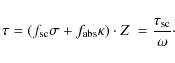 |
(4) |
The basic model grid (Sect. 3) considers only Rayleigh scattering (
2.3 Geometric parameters
The geometric parameters describe the location of the considered
surface point P and the escape direction of the photons (Fig. 1).
A global coordinate system describes the orientation of the planet with respect to the star. Its polar axis is the surface normal at the sub-stellar point S', and the location of each point P is described by polar angle ![]() and azimuthal angle
and azimuthal angle ![]() (not drawn).
(not drawn). ![]() is also the photon's angle of incidence at point P. The escape direction, i.e. the location of the observer, is given by a polar angle
is also the photon's angle of incidence at point P. The escape direction, i.e. the location of the observer, is given by a polar angle ![]() and azimuthal angle
and azimuthal angle ![]() (not drawn).
(not drawn). ![]() is equivalent to the phase angle defined by the three (central) points: star or sun S, planet 0, and observer E (Earth).
is equivalent to the phase angle defined by the three (central) points: star or sun S, planet 0, and observer E (Earth).
For the description of the scattering processes, a local coordinate system is set up at point P for the plane parallel atmosphere with surface normal z perpendicular to the planet surface in P, polar angle ![]() and azimuthal angle
and azimuthal angle ![]() .
.
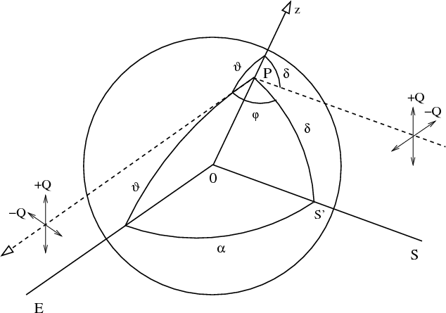 |
Figure 1: Model geometry. The dashed line represents the trajectory of a reflected photon. |
| Open with DEXTER | |
In general, each point P can have individual atmospheric properties. Then
the model outputs, the Stokes vector components I, Q and U, depend each on seven parameters:
This description allows calculation of the reflected intensity and polarization of each surface point on the illuminated hemisphere viewed from any direction. Obviously this large parameter space needs to be simplified for a first parameter analysis. If we adopt the same atmospheric structure everywhere on the planet,
For extrasolar planets it will not be
possible to resolve the disk in the near future. For disk-integrated results we can eliminate the dependence
of the reflected intensity and polarization on the surface point parameters ![]() and
and ![]() .
Because of the rotational symmetry of the geometric model, the
intensity and the polarization then only depend on the polar
viewing angle or phase angle
.
Because of the rotational symmetry of the geometric model, the
intensity and the polarization then only depend on the polar
viewing angle or phase angle ![]() .
Moreover the orientation of the
polarization signal is either parallel or perpendicular to the scattering
plane (the plane S-0-E), which we call the Qpolarization direction. Q is defined positive for a polarization
perpendicular to the plane S-0-E and negative for a polarization parallel to this
plane. The U-polarization is zero in this coordinate system for
symmetry reasons.
.
Moreover the orientation of the
polarization signal is either parallel or perpendicular to the scattering
plane (the plane S-0-E), which we call the Qpolarization direction. Q is defined positive for a polarization
perpendicular to the plane S-0-E and negative for a polarization parallel to this
plane. The U-polarization is zero in this coordinate system for
symmetry reasons.
For the full disk the integrated intensity and polarization signals from a planet
depend on the following parameters:
For solar system planets at opposition we obtain a rotationally symmetric scattering geometry (viewing direction is identical to the axis of symmetry of the geometric model). We then have a scattering model which depends only on
For exact opposition the dependences of the scattering model results
can be described by the following parameters:
These are the center to limb intensity curve and the center to limb radial polarization curves which both depend only on the atmospheric parameters.
2.4 Monte Carlo simulations
For our simulations we used the Monte Carlo code described in Schmid
(1992), which was slightly adapted for the case of light reflection
from a planet. Basically the code calculates the random
walk histories of many photons in the planet model atmosphere until the photons have
escaped or are destroyed by an absorption process. After a sufficiently large
number have escaped, the scattering intensity and polarization of the
reflected light can be established for different lines of sight.
In our calculations we assume that despite multiple scatterings the escaping
photons emerge at the same point where they penetrated into the planet.
In each scattering process the photon undergoes a
direction and polarization change calculated from the appropriate phase matrix.
The linear polarization of the photons in the simulations is defined by the
orientation ![]() of the electric vector for the photon's
electromagnetic wave. In a given coordinate system we can then
evaluate the contribution to the Stokes intensity for each photon in
of the electric vector for the photon's
electromagnetic wave. In a given coordinate system we can then
evaluate the contribution to the Stokes intensity for each photon in
![]() and
and
![]() direction.
direction.
The escaping photons have to be collected in discret
direction bins (in our models phase angles
![]() with a finite bin width
with a finite bin width
![]() )
to evaluate
)
to evaluate ![]() and
and ![]() .
These are then a mean photon intensity and polarization for that bin.
.
These are then a mean photon intensity and polarization for that bin.
![]() should be small to resolve any structure in
should be small to resolve any structure in ![]() and
and ![]() ,
but also sufficiently large to collect enough photons for results with small statistical
errors. The aim of our simulations is to reach at least the expected
precision of observational data. The rotational
symmetry imposed on our models helps to increase the bin size for the phase curve
interval
,
but also sufficiently large to collect enough photons for results with small statistical
errors. The aim of our simulations is to reach at least the expected
precision of observational data. The rotational
symmetry imposed on our models helps to increase the bin size for the phase curve
interval ![]() ,
which behaves like
,
which behaves like
![]() .
This means that we have to divide the photon count per bin
by the factor
.
This means that we have to divide the photon count per bin
by the factor
![]() .
The intensity is obtained by normalizing with the reflectivity of a white Lambertian disk.
For a given simulation the relative statistical
errors (photon shot noise) are particularly good for
.
The intensity is obtained by normalizing with the reflectivity of a white Lambertian disk.
For a given simulation the relative statistical
errors (photon shot noise) are particularly good for
![]() ,
much less favorable for
,
much less favorable for
![]() and very bad for
and very bad for
![]() where only a few photons
will be collected, because the irradiated hemisphere of the planet
is almost invisible for this phase angle. For the center-to-limb curves we bin uniformly in
where only a few photons
will be collected, because the irradiated hemisphere of the planet
is almost invisible for this phase angle. For the center-to-limb curves we bin uniformly in
![]() with a bin size of
with a bin size of
![]() ,
which requires an additional normalization by
,
which requires an additional normalization by
![]() .
.
The number of photons per model was chosen such that the
number of reflected photons in phase angle bins relevant for observations (
![]() )
are about
)
are about
![]() when integrated over the whole disk. This corresponds to an error in polarization
when integrated over the whole disk. This corresponds to an error in polarization
![]() %. For the radial curves the total number of photons was increased such that the same precision was reached in most radial bins. No photons emerge at the exact phase angle
%. For the radial curves the total number of photons was increased such that the same precision was reached in most radial bins. No photons emerge at the exact phase angle
![]() .
Therefore for the limb polarization calculations we count all photons that are in the bin
.
Therefore for the limb polarization calculations we count all photons that are in the bin
![]() ,
even though the calculation for the radial polarization includes the assumption that
,
even though the calculation for the radial polarization includes the assumption that
![]() .
The error induced by this measure is smaller than the statistical error.
.
The error induced by this measure is smaller than the statistical error.
A general guideline for the Monte Carlo technique for random walk problems is given in Cashwell & Everett (1959) and many Monte Carlo simulations for the investigation of light scattering are described in the astronomical literature (see e.g. Witt 1991; Code & Whitney 1995; Wolf et al. 1999). In Schmid (1992) a detailed description on many aspects of the employed Monte Carlo code are given; e.g. the general scheme of the code, the required transformations between the involved coordinate systems (star-planet, planet-plane parallel atmosphere, atmosphere-photon), the determination of the free path length, the treatment of isotropic scattering and Rayleigh scattering according to the Rayleigh phase matrix, an assessment of statistical errors, and a comparison with analytical calculations.
3 Model results for a homogeneous Rayleigh scattering atmosphere
This section discusses the model grid results for simple homogeneous Rayleigh scattering atmospheres described by parameters ![]() ,
,
![]() and
and ![]() (cf. Sect. 2.2) We discuss phase curves (Sect. 3.1) and radial profiles (Sect. 3.2) for selected cases and explore the full parameter space for disk-integrated results at
(cf. Sect. 2.2) We discuss phase curves (Sect. 3.1) and radial profiles (Sect. 3.2) for selected cases and explore the full parameter space for disk-integrated results at
![]() and
and
![]() (Sect. 3.3).
(Sect. 3.3).
Many of the general dependences of these model results on atmospheric parameters were already discussed in previous studies mentioned in the introduction (Sect. 1). Compared to these our calculations are much more comprehensive and the extensive model grid results are provided in electronic form (see Appendix A). An overview of the dependence of observable quantities, such as intensity, fractional polarization and polarized intensity, on atmosphere parameters is presented in diagrams which may be useful for the interpretation of observational data.
The results presented in this section are in very good agreement with the previous calculations in Kattawar & Adams (1971), Stam et al. (2006) and Schmid et al. (2006a).
3.1 Phase curves
![\begin{figure}
\par\includegraphics[width=17cm,clip]{11760f02.eps} \end{figure}](/articles/aa/full_html/2009/34/aa11760-09/img102.png) |
Figure 2:
Left: phase dependence of the intensity I, fractional
polarization q and polarized intensity Q for Rayleigh
scattering atmospheres. Right: radial dependence of the intensity I, radial
polarization qr and radial polarized intensity Qr at
opposition. Line styles denote: semi-infinite case
|
| Open with DEXTER | |
For the investigation of extrasolar planets, the phase dependence of the disk-integrated polarization is of interest. We discuss the phase curve for selected model cases (Fig. 2, left): a semi-infinite and a finite scattering layer with different absorption properties of the scattering and surface layers.
The semi-infinite, conservatively scattering layer is a good reference case for an illuminated sphere and is often used for scattering atmospheres. All irradiated light is reflected after one or several scatterings and the spherical albedo is equal to 1. An intensity phase curve for isotropic scattering is given in van de Hulst (1980), and Bhatia & Abhyankar (1982) published a polarization curve for Rayleigh scattering in graphical form, but no tabulated values could be found in the literature.
In our Monte Carlo simulation we treat
the semi-infinite atmosphere as
![]() and
and
![]() ,
which yields essentially the same
results as an infinite layer but avoids infinite scattering of some
photons. Our results of this case are tabulated in Table 1.
,
which yields essentially the same
results as an infinite layer but avoids infinite scattering of some
photons. Our results of this case are tabulated in Table 1.
Table 1:
Reflectivity ![]() ,
polarization fraction
,
polarization fraction ![]() and polarized intensity
and polarized intensity ![]() phase curves for a very deep
(
phase curves for a very deep
(![]() )
conservative
)
conservative
![]() Rayleigh scattering atmosphere above a perfectly
reflecting Lambert surface (surface albedo
Rayleigh scattering atmosphere above a perfectly
reflecting Lambert surface (surface albedo
![]() ).
).
Intensity:
The intensity phase curves
Of course, the reflected intensity decreases with absorption
(with lower single scattering albedo ![]() )
in the atmosphere and with
the albedo
)
in the atmosphere and with
the albedo ![]() of the underlying surface layer. The effect of
absorption in the scattering atmosphere is important for thick layers,
while the albedo of the underlying surface is important if the optical
depths of the scattering region above is small. A quantitative
description of these dependences is given in Dlugach & Yanovitskij (1974) and Sromovsky (2005b).
of the underlying surface layer. The effect of
absorption in the scattering atmosphere is important for thick layers,
while the albedo of the underlying surface is important if the optical
depths of the scattering region above is small. A quantitative
description of these dependences is given in Dlugach & Yanovitskij (1974) and Sromovsky (2005b).
Polarization fraction.
The disk-integrated polarization fraction
The polarization for the semi-infinite, conservative Rayleigh scattering layer
reaches a maximum of q=32.6% for
![]() .
For reduced scattering albedo, e.g. due to absorption in a molecular band,
.
For reduced scattering albedo, e.g. due to absorption in a molecular band, ![]() increases (see e.g. van de Hulst 1980). This happens because absorption strongly
reduces the fraction of multiply scattered photons in the reflected light which have randomized
polarization directions. If the absorption is
very strong then the reflected light consists essentially only
of photons that made one single Rayleigh scattering. The polarization phase curve
then approaches the Rayleigh scattering
polarization phase function
increases (see e.g. van de Hulst 1980). This happens because absorption strongly
reduces the fraction of multiply scattered photons in the reflected light which have randomized
polarization directions. If the absorption is
very strong then the reflected light consists essentially only
of photons that made one single Rayleigh scattering. The polarization phase curve
then approaches the Rayleigh scattering
polarization phase function
![]() with a polarization close to 100 % at
with a polarization close to 100 % at
![]() .
.
For finite scattering atmospheres the polarization fraction qalso depends on the albedo of the surface layer. In the models discussed in this section the polarization is only produced in the Rayleigh scattering layer, while reflection from the surface layer is unpolarized. Therefore the resulting polarization is low for a high surface albedo and high for a low surface albedo (see e.g. Kattawar & Adams 1971; Stam 2008). This reflects the relative contribution of the polarized light from the scattering layer with respect to the unpolarized light reflected from the surface underneath.
The peak of the polarization curve is shifted towards large phase
angles (
![]() )
for models with thin scattering layers and
high surface albedos, as previously described by Kattawar & Adams
(1971). At large
phase angles (
)
for models with thin scattering layers and
high surface albedos, as previously described by Kattawar & Adams
(1971). At large
phase angles (
![]() ), when only a planet crescent is visible, the fraction of
scattered photons hitting the planet initially under grazing
incidence is relatively high. For a thin scattering layer grazing
incidence helps to enhance the probability for a polarizing Rayleigh scattering.
For this reason the polarized
light from the Rayleigh scattering atmosphere is less diluted by
unpolarized light reflected from the surface at large phase angles and
the fractional polarization is higher.
), when only a planet crescent is visible, the fraction of
scattered photons hitting the planet initially under grazing
incidence is relatively high. For a thin scattering layer grazing
incidence helps to enhance the probability for a polarizing Rayleigh scattering.
For this reason the polarized
light from the Rayleigh scattering atmosphere is less diluted by
unpolarized light reflected from the surface at large phase angles and
the fractional polarization is higher.
Polarized intensity.
The polarized intensityThe polarized intensity decreases with increasing absorption, because the drop in intensity is stronger than the increase in fractional polarization. The polarization flux is a rough measure for the number of reflected photons undergoing one single Rayleigh scattering. Second and higher order scatterings also add to the polarized intensity, but only at a much lower level. Adding absorption can only reduce the number of such scatterings and therefore diminishes the polarized intensity.
A very important property of the polarization flux Q is that it
does not depend on the albedo of the surface layer ![]() (assumed to produce no
polarization) below the scattering region.
(assumed to produce no
polarization) below the scattering region.
3.2 Radial dependence for resolved planetary disks at opposition
For the interpretation of the limb polarization of solar system objects close to opposition, we discuss the radial or center-to-limb dependence of the intensity I(r), the radial polarization qr(r) and the radial polarized intensity Qr(r) (Fig. 2, right) for the same model parameters as for the phase curves in Sect. 3.1.
Intensity:
The radial intensity curve I(r) shows a pronounced limb darkening in the semi-infinite conservative case. For a strongly absorbing atmosphere, e.g. within an absorption band, the I(r)-curve becomes essentially flat. Thus for an absorbing (and homogeneous) semi-infinite atmosphere limb brightening cannot be produced. For comparison the center-to-limb intensity curve I(r) for isotropic scattering and for a Lambert sphere (
For finite scattering atmospheres with an optically thin layer the
center-to-limb intensity curve can show a limb brightening
effect. Limb brightening occurs for a highly reflective scattering
layer (high ![]() )
located above a dark surface (low
)
located above a dark surface (low ![]() ), e.g. a thin aerosol layer or a methane-poor layer above the methane-rich absorbing layer (e.g. Price 1978). Limb brightening is observed in solar system planets in deep absorption band (e.g. Karkoschka 2001; Sromovsky & Fry 2007). Limb brightening is investigated in more detail in Sect. 3.2.1.
), e.g. a thin aerosol layer or a methane-poor layer above the methane-rich absorbing layer (e.g. Price 1978). Limb brightening is observed in solar system planets in deep absorption band (e.g. Karkoschka 2001; Sromovsky & Fry 2007). Limb brightening is investigated in more detail in Sect. 3.2.1.
Radial polarization fraction:
The radial polarization fraction qr(r) is always zero in the disk center because of the symmetry of the scattering situation. For all cases the polarization increases steadily towards the limb and reaches a maximum value close to the limb between r=0.95 and 1.0. The polarization qr(r) is always positive, which means a radial polarization direction or limb polarization perpendicular to the limb.
It is important to note that the limb polarization decreases with
decreasing single scattering albedo ![]() (more absorption) in
contrast to the situation at large phase angles.
This indicates that the photons producing the limb
polarization are more strongly reduced by
absorption than the reflected ``unpolarized'' photons.
(more absorption) in
contrast to the situation at large phase angles.
This indicates that the photons producing the limb
polarization are more strongly reduced by
absorption than the reflected ``unpolarized'' photons.
The explanation is that singly scattered (i.e. backscattered) photons
do not contribute to the limb
polarization, while reflected photons scattered twice or a few times are responsible
for the largest part of the limb polarization. Absorption implies
that a larger fraction of escaping photons are singly-scattered and therefore
unpolarized at opposition. Note however that for the semi-infinite atmosphere,
the maximum radial polarization is not reached in the conservative
case. A slightly lower scattering albedo (
![]() )
mostly reduces the amount of highest order scatterings
and thus the polarization fraction is somewhat enhanced when
compared to the conservative case
(see Schmid et al. 2006a,
and Fig. 7 in Sect. 3.3).
)
mostly reduces the amount of highest order scatterings
and thus the polarization fraction is somewhat enhanced when
compared to the conservative case
(see Schmid et al. 2006a,
and Fig. 7 in Sect. 3.3).
The fractional limb polarization qr(r) for finite scattering layers depends
strongly on the albedo of the underlying surface ![]() :
qr(r) is high for low
:
qr(r) is high for low ![]() and low for high
and low for high ![]() like for large phase angles.
A low surface albedo decreases the photons with multiple scatterings in the plane perpendicular to the limb, which are polarized parallel to the limb, thus enhancing the polarization in perpendicular direction. Therefore the limb polarization of a bright layer over a dark one can be even higher than for a semi-infinite atmosphere. This is discussed in more detail in Sect. 3.3.
like for large phase angles.
A low surface albedo decreases the photons with multiple scatterings in the plane perpendicular to the limb, which are polarized parallel to the limb, thus enhancing the polarization in perpendicular direction. Therefore the limb polarization of a bright layer over a dark one can be even higher than for a semi-infinite atmosphere. This is discussed in more detail in Sect. 3.3.
Radial polarized intensity:
The radial polarized intensity
For finite atmospheres, the limb polarization flux Qr(r)
depends only slightly on the surface albedo. Decreasing ![]() from 1 to 0 can increase Qr(r) at most
from 1 to 0 can increase Qr(r) at most
![]() for some models, while for most models Qr(r) is virtually constant. This is similar to the case for large phase angles.
for some models, while for most models Qr(r) is virtually constant. This is similar to the case for large phase angles.
3.2.1 Limb darkening and limb brightening vs. limb polarization
For a surface with a low albedo ![]() below a thin scattering layer the limb can be brighter than the disk
center, an effect that is generally called limb brightening. In principle this effect should be
called ``a central disk darkening'', because the low surface albedo
below a thin scattering layer the limb can be brighter than the disk
center, an effect that is generally called limb brightening. In principle this effect should be
called ``a central disk darkening'', because the low surface albedo ![]() does not brighten the limb.
It only absorbs more light in the center of the disk, where a higher fraction of
photons reach the absorbing surface because of their perpendicular
incidence when compared to the situation of grazing incidence at the limb.
Despite this fact we will retain the term ``limb brightening'' and consider the
limb brightness on a relative scale compared to the brightness of the
disk center.
does not brighten the limb.
It only absorbs more light in the center of the disk, where a higher fraction of
photons reach the absorbing surface because of their perpendicular
incidence when compared to the situation of grazing incidence at the limb.
Despite this fact we will retain the term ``limb brightening'' and consider the
limb brightness on a relative scale compared to the brightness of the
disk center.
The limb darkening and limb brightening effect can be parametrized to a first order using the Minnaert law I(r) = Ir=0 (1-r2)k-1/2. The Minnaert parameter k determines the shape of the curve, k=1 corresponds to Lambert's law, k=0.5 to a flat intensity distribution I(r) = I0 and k < 0.5to limb brightening. The k parameter was determined by fitting Minnaert's law to all modeled intensity profiles, fixing the intensity at the center and excluding the outermost point where the formula diverges for k<0.5. With the exception of some cases mentioned below, most profiles can be fitted adequatly.
In Fig. 3 different examples of limb darkening and
limb brightening are shown along with the best fit of the Minnaert
law. Intensities are normalized to the central disk intensity.
There are two types of limb brightening curves. For very thin
atmospheres the maximal brightness is measured at the very edge of the
planet, while for a moderate optical depth the intensity raises slightly up to
a certain radius (e.g. 0.9 Rp) and then drops very close to the
limb. This second case cannot be fitted with the one-parameter
Minnaert law and is approximated here by a relatively flat curve
![]() .
.
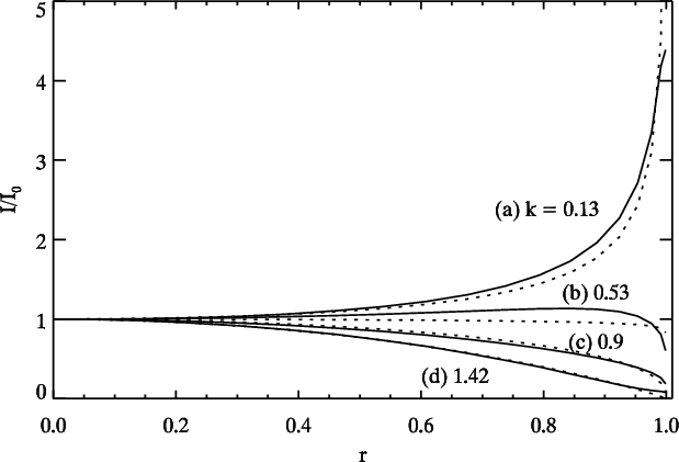 |
Figure 3:
Radial intensity curves for different model parameters normalized to the central disk intensity, showing examples of limb darkening and limb brightening. The solid line is the calculated model and the dotted line the best fit with the Minnaert law. (a), (b) and (c) are for conservatively ( |
| Open with DEXTER | |
The limiting case of a conservative semi-infinite atmosphere yields a Minnaert parameter of
![]() .
For
.
For ![]() going towards 0, k tends to a flat intenstiy distribution k=0.5. For finite atmospheres there
is a strong dependence on the surface albedo
going towards 0, k tends to a flat intenstiy distribution k=0.5. For finite atmospheres there
is a strong dependence on the surface albedo ![]() .
For a strongly absorbing atmosphere over a bright surface (
.
For a strongly absorbing atmosphere over a bright surface (![]() low,
low,
![]() high) absorption is more likely towards the limb (k > 1), for a bright atmosphere
over a dark surface the opposite is true (k < 0.5). In the latter case the central disk intensity
is very low.
high) absorption is more likely towards the limb (k > 1), for a bright atmosphere
over a dark surface the opposite is true (k < 0.5). In the latter case the central disk intensity
is very low.
Similar to limb brightening, the limb polarization is also enhanced for a bright scattering layer over a dark surface. However, there are fundamental differences between these two effects. Limb polarization arises only for a polarizing process like Rayleigh scattering, while limb brightening occurs also for non-polarizing scattering processes like isotropic scattering. Additionally limb brightening is the stronger the thinner the upper bright layer, while limb polarization requires a sufficiently thick scattering layer above the dark surface. Finally, limb polarization can also occur for cases of limb darkening, e.g. the semi-infinite, conservative atmosphere. Therefore, the two effects provide complementary diagnostics of the vertical structure of the atmosphere.
3.3 Parameter study for quadrature phase
 and opposition

This section explores the full parameter space for
simple Rayleigh scattering atmospheres. We explore the parameter space by varying one of the three parameters ![]() ,
,
![]() and
and ![]() (cf. Sect. 2.2) while fixing the other two. We study the resulting intensity
(cf. Sect. 2.2) while fixing the other two. We study the resulting intensity
![]() ,
polarization fraction
,
polarization fraction
![]() ,
and polarized intensity
,
and polarized intensity
![]() (Figs. 4 to 6).
(Figs. 4 to 6).
The shapes of the model phase curves for the intensity ![]() ,
fractional polarization
,
fractional polarization ![]() ,
and polarized intensity
,
and polarized intensity ![]() look very similar for different
model parameters (see Fig. 2).
Therefore it is reasonable for a model parameter study to select
the results for the phase angle
look very similar for different
model parameters (see Fig. 2).
Therefore it is reasonable for a model parameter study to select
the results for the phase angle
![]() ,
considering them as representative (qualitatively) for all phase angles.
A phase angle
,
considering them as representative (qualitatively) for all phase angles.
A phase angle
![]() is ideal for extrasolar planets because all
planets will pass through this configuration twice during an orbit,
regardless of inclination.
is ideal for extrasolar planets because all
planets will pass through this configuration twice during an orbit,
regardless of inclination.
The same type of parameter study is presented for the limb
polarization of planets at opposition (
![]() ). For this we determine
disk-integrated (averaged) quantities for the intensity
and radial polarization from the model results (Figs. 7 to 9). The integrated intensity
). For this we determine
disk-integrated (averaged) quantities for the intensity
and radial polarization from the model results (Figs. 7 to 9). The integrated intensity
![]() is
equivalent to the geometric albedo,
is
equivalent to the geometric albedo,
![]() is the
intensity weighted average of the fractional polarization,
and
is the
intensity weighted average of the fractional polarization,
and
![]() the
integrated polarized intensity on the same scale as the integrated
intensity. These quantities are determined as described in
Sect. 2.1.
the
integrated polarized intensity on the same scale as the integrated
intensity. These quantities are determined as described in
Sect. 2.1.
Figures 4 and 7 show the dependence
on the single scattering albedo ![]() .
For a given scattering
optical depth
.
For a given scattering
optical depth
![]() a reduction in
a reduction in ![]() is equivalent to an
enhancement of the absorption
is equivalent to an
enhancement of the absorption ![]() in the scattering layer.
Strong differences in
in the scattering layer.
Strong differences in
![]() occur in planetary atmospheres for
molecular absorptions (e.g. due to CH4 or H2O) inside and
outside the band while
occur in planetary atmospheres for
molecular absorptions (e.g. due to CH4 or H2O) inside and
outside the band while ![]() is essentially equal.
is essentially equal.
In Figs. 5 and 8 the Rayleigh
scattering optical depths from
![]() to 0.01 are plotted.
This illustrates quite well the possible
spectral dependence from short to long wavelengths (left to right)
for a Rayleigh scattering atmosphere. Since the Rayleigh
scattering cross sections is proportional to
to 0.01 are plotted.
This illustrates quite well the possible
spectral dependence from short to long wavelengths (left to right)
for a Rayleigh scattering atmosphere. Since the Rayleigh
scattering cross sections is proportional to
![]() ,
it is
possible that a planet has
,
it is
possible that a planet has
![]() at 400 nm and
at 400 nm and
![]() at 800 nm.
at 800 nm.
The effect of the albedo ![]() of the surface below the Rayleigh
scattering layer is shown in Figs. 6 and
9.
of the surface below the Rayleigh
scattering layer is shown in Figs. 6 and
9.
General results from Figs. 4 to 9 are:
- lowering the Rayleigh scattering albedo
always results in a lower intensity I, and lower
polarized intensity Q or Qr;
- lowering the Rayleigh scattering albedo
results in a
higher polarization q at large phase angles. Contrary to this the
fractional limb polarization qr is reduced for lower ;
- lowering the Rayleigh scattering optical depth
produces a strong reduction in
the polarized intensity Q or Qr in the optically thin case
 and causes
essentially no change in Q or Qr in the optical thick case
and causes
essentially no change in Q or Qr in the optical thick case
 ;
;
- lowering the surface albedo
lowers the intensity I and
enhances the fractional polarization q or qr;
- changing the surface albedo
does not change the
polarized flux Q and hardly Qr.
Another difference is the influence of
![]() on the
fractional polarization: q drops with
on the
fractional polarization: q drops with
![]() for bright non-polarizing
surfaces and increases for dark surfaces. It is more complicated at opposition: the limb polarization is highest if the dark ground eliminates photons that would otherwise scatter twice perpendicular to the limb, but the atmosphere is still thick
enough to produce many photons that escape having scattered twice parallel to the limb.
The maximum possible limb polarization
for bright non-polarizing
surfaces and increases for dark surfaces. It is more complicated at opposition: the limb polarization is highest if the dark ground eliminates photons that would otherwise scatter twice perpendicular to the limb, but the atmosphere is still thick
enough to produce many photons that escape having scattered twice parallel to the limb.
The maximum possible limb polarization
![]() % is reached for
% is reached for
![]() ,
,
![]() and
and ![]() .
.
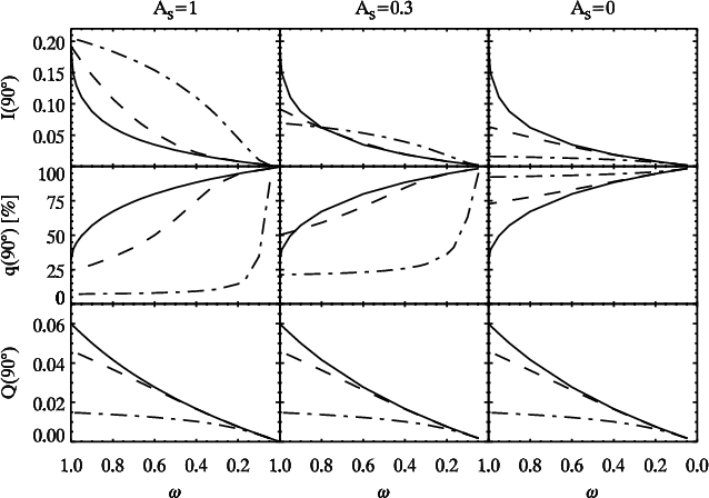 |
Figure 4:
Intensity, polarization and polarized intensity at quadrature as function of single scattering albedo |
| Open with DEXTER | |
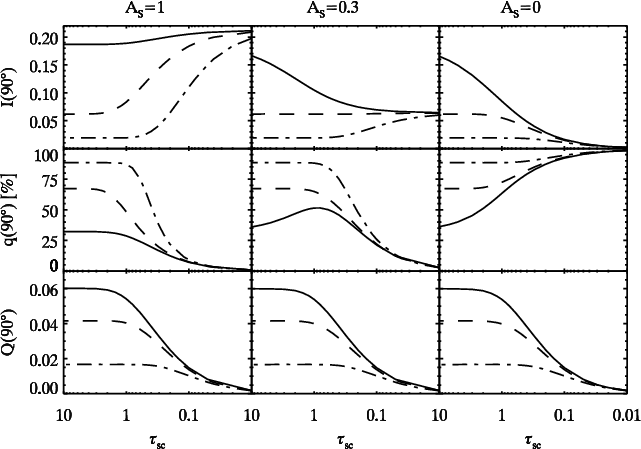 |
Figure 5:
Intensity, polarization and polarized intensity at quadrature as function of optical depth
|
| Open with DEXTER | |
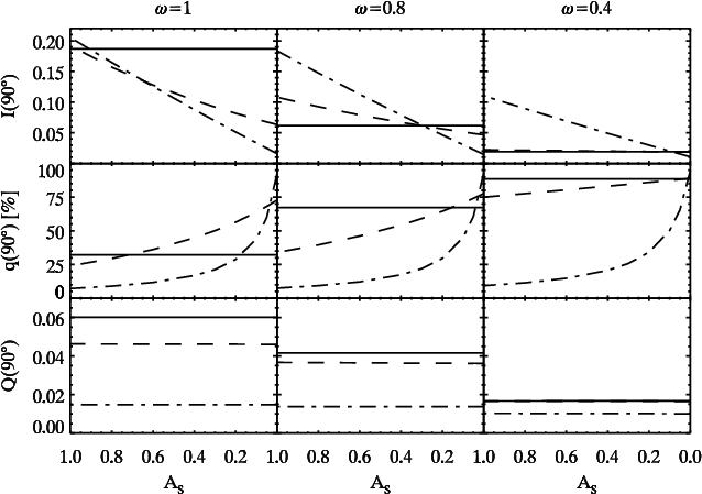 |
Figure 6:
Intensity, polarization and polarized intensity at quadrature as function of surface albedo |
| Open with DEXTER | |
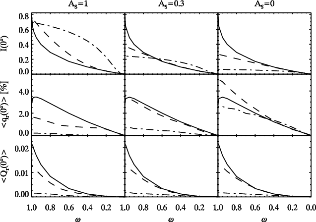 |
Figure 7:
Geometric albedo, disk-integrated radial polarization and polarized intensity at opposition as function of single scattering albedo |
| Open with DEXTER | |
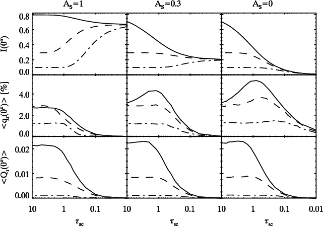 |
Figure 8:
Geometric albedo, disk-integrated radial polarization and polarized intensity at opposition as function of optical depth
|
| Open with DEXTER | |
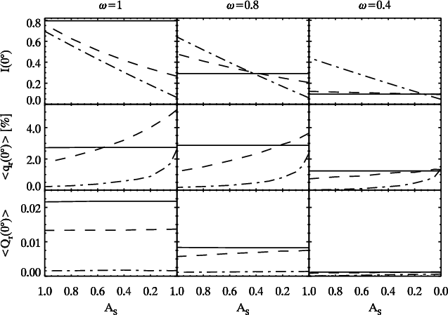 |
Figure 9:
Geometric albedo, disk-integrated radial polarization and polarized intensity at opposition as function of surface albedo |
| Open with DEXTER | |
From the variation of
![]() shown in Fig. 5 it can
be seen that the polarized intensity
shown in Fig. 5 it can
be seen that the polarized intensity
![]() saturates above
saturates above
![]() .
Therefore
.
Therefore
![]() cannot probe deep atmospheric layers.
For the intensity and fractional polarization, an absorbing ground under a conservatively
scattering layer can be noticed even at
cannot probe deep atmospheric layers.
For the intensity and fractional polarization, an absorbing ground under a conservatively
scattering layer can be noticed even at
![]() .
.
The polarized intensity ![]() consists mostly of photons undergoing just one single Rayleigh scattering. Therefore, Q is not
changed by processes which happen deep in the atmosphere or by diffuse scattering on the surface. Q is only reduced if the number of single Rayleigh scatterings are reduced, e.g. because there is only a thin Rayleigh scattering layer or photons are efficiently absorbed high in the
atmosphere.
consists mostly of photons undergoing just one single Rayleigh scattering. Therefore, Q is not
changed by processes which happen deep in the atmosphere or by diffuse scattering on the surface. Q is only reduced if the number of single Rayleigh scatterings are reduced, e.g. because there is only a thin Rayleigh scattering layer or photons are efficiently absorbed high in the
atmosphere.
We can approximate the polarized intensity Q
by the following parametrization:
where ![]() and
and
![]() are fit parameters. Table 2 shows the best fit parameter
are fit parameters. Table 2 shows the best fit parameter
![]() ,
while
,
while
![]() and
and ![]() are listed in Table 1.
are listed in Table 1.
Table 2:
Best fit parameter
![]() for the parametrization of the polarized intensity Q (Eq. (5)).
for the parametrization of the polarized intensity Q (Eq. (5)).
For optically thick Rayleigh scattering atmospheres the polarized intensity
Q depends only on the single scattering albedo ![]() ,
and the parametrization reduces to:
,
and the parametrization reduces to:
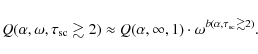
At quadrature this is
 |
(7) |
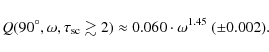
For the limb polarization flux
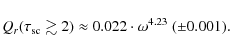 |
(8) |
4 Models beyond a Rayleigh scattering layer with a Lambert surface
The three parameter model grid discussed in Sect. 3.3 provides an overview on basic dependences of simple Rayleigh scattering models. In this section we describe a few results for particle scattering properties different from pure Rayleigh scattering, or models with more than one polarizing scattering layer.
4.1 Atmospheres with Rayleigh and isotropic scattering
Pure Rayleigh scattering is a simplification for planetary atmospheres. Already for Rayleigh scattering by molecular hydrogen one needs to account for a weak depolarization effect, because the diatomic molecule is non-spherical. Another depolarization effect for scattered radiation occurs in dense gas because collisions with other particles take place frequently during the scattering process. In addition aerosols and dust particles can also be efficient scatterers in planetary atmospheres and the net scattering phase matrix differs from Rayleigh scattering and should be evaluated, e.g. by using the more general Mie theory.
A simple way for taking such effects into account in a first approximation is to use a linear combination of
the Rayleigh scattering and isotropic scattering phase matrices
| (9) |
where
Isotropic scattering is non-polarizing. If the scattering in the atmosphere is composed of both isotropic and Rayleigh scattering, then the fractional polarization and the polarized intensity are reduced by isotropic scattering, while the intensity is comparable (cf. Fig. 2).
Figure 10 shows the fractional
polarization
![]() at quadrature as a function of
at quadrature as a function of
![]() for a few representative cases. In the single scattering limit the
decrease is linear, the strongest deviation from a linear law is found for the semi-infinite
atmosphere because of the large amount of multiple scatterings. A similar behavior is found for other phase
angles, as well as for the radial limb polarization at opposition.
for a few representative cases. In the single scattering limit the
decrease is linear, the strongest deviation from a linear law is found for the semi-infinite
atmosphere because of the large amount of multiple scatterings. A similar behavior is found for other phase
angles, as well as for the radial limb polarization at opposition.
![\begin{figure}
\par\includegraphics[width=8.5cm,clip]{11760f10.eps}
\end{figure}](/articles/aa/full_html/2009/34/aa11760-09/img164.png) |
Figure 10:
Polarization of atmospheres with Rayleigh and isotropic scattering at 90 |
| Open with DEXTER | |
4.2 Forward-scattering phase functions
The high polarization of Jupiter's poles and the disk-integrated polarization of Titan (e.g. Tomasko & Smith 1982; Smith & Tomasko 1984) has been explained by the presence of a thick layer of polarizing haze particles. The derived single scattering properties indicate strong forward scattering and Rayleigh-like linear polarization with maximal polarization close to 100% at about 90![]() scattering angle. Particles that satisfy this behavior are thought to be aggregates that are non-spherical and with a projected area smaller than optical wavelengths (e.g. West 1991). We investigate the polarization properties of a planet with such a haze layer. The particle scattering properties are implemented as described in Braak et al. (2002) using a simple parametrized scattering matrix of the form
scattering angle. Particles that satisfy this behavior are thought to be aggregates that are non-spherical and with a projected area smaller than optical wavelengths (e.g. West 1991). We investigate the polarization properties of a planet with such a haze layer. The particle scattering properties are implemented as described in Braak et al. (2002) using a simple parametrized scattering matrix of the form
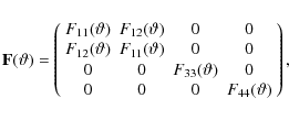 |
(10) |
where
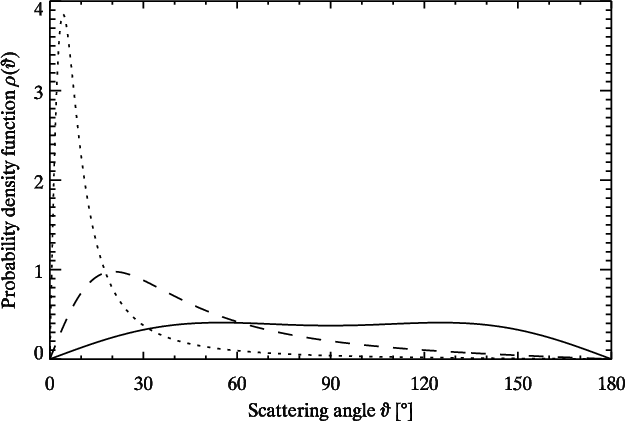 |
Figure 11:
Probability density function
|
| Open with DEXTER | |
Figure 11 shows the probability density function
![]() for
for
![]() in comparison with Rayleigh scattering. The probability density function for the scattering angle
in comparison with Rayleigh scattering. The probability density function for the scattering angle ![]() is the phase function
is the phase function
![]() weighted by
weighted by
![]() and normalized such that the integral over
and normalized such that the integral over
![]() equals 1. From this function the probability of the scattering angle within a certain interval is calculated by integrating
equals 1. From this function the probability of the scattering angle within a certain interval is calculated by integrating
![]() over this interval. One can see that for the haze models small scatttering angles (foward scattering) are greatly enhanced in comparison to Rayleigh scattering, while the probability for backscattering is much lower.
over this interval. One can see that for the haze models small scatttering angles (foward scattering) are greatly enhanced in comparison to Rayleigh scattering, while the probability for backscattering is much lower.
![]() describes the fractional polarization of the scattered radiation as a function of the scattering angle. For scattering on haze particles it can be similar to Rayleigh scattering scaled by a factor pm, the maximal single scattering polarization at
describes the fractional polarization of the scattered radiation as a function of the scattering angle. For scattering on haze particles it can be similar to Rayleigh scattering scaled by a factor pm, the maximal single scattering polarization at ![]() scattering angle. For a first qualitative analysis we set pm=1 which is an upper limit that may slightly overestimate the resulting polarization. The other matrix elements are identical to Rayleigh scattering.
scattering angle. For a first qualitative analysis we set pm=1 which is an upper limit that may slightly overestimate the resulting polarization. The other matrix elements are identical to Rayleigh scattering.
Figures 12 and 13 show the phase and radial dependences for the haze models similar to the Rayleigh scattering case in Sects. 3.1 and 3.2.
Intensity:
The phase curves of the haze models differ from the Rayleigh scattering models mainly at small phase angles. The geometric albedo is lower for the haze models because backscattering is strongly suppressed compared to Rayleigh scattering. This is already discussed by Dlugach & Yanovitskij (1974), who calculated albedos for semi-infinite hazy atmospheres. Our calculations result in slightly higher albedos because of the inclusion of polarization. At phase angles around 90 ![\begin{figure}
\par\includegraphics[width=18.8cm,clip]{11760f12.eps}
\end{figure}](/articles/aa/full_html/2009/34/aa11760-09/img175.png) |
Figure 12:
Phase dependence of the intensity I, fractional
polarization q and polarized intensity Q for a haze layer. Left: semi-infinite case
|
| Open with DEXTER | |
![\begin{figure}
\par\includegraphics[width=18.8cm,clip]{11760f13.eps}
\end{figure}](/articles/aa/full_html/2009/34/aa11760-09/img176.png) |
Figure 13:
Radial dependence of the intensity I, radial
polarization qr and radial polarized intensity Qr at
opposition for a haze layer. Left: semi-infinite case
|
| Open with DEXTER | |
Polarization fraction:
The angle of maximal polarization is generally larger for the haze models than for Rayleigh scattering. In the semi-infinite conservative case it is
Polarized intensity:
The polarized intensity
4.3 Models with two polarizing layers
Up to now we have treated the region below the scattering layer
simply as a Lambert surface with an albedo ![]() ,
which
produces no polarization. In this section we explore model results for
two polarizing layers with different absorption properties, where the lower layer can be a
semi-infinite Rayleigh scattering atmosphere as described in
Sect. 3.1.
,
which
produces no polarization. In this section we explore model results for
two polarizing layers with different absorption properties, where the lower layer can be a
semi-infinite Rayleigh scattering atmosphere as described in
Sect. 3.1.
We focus on the question at what depth of the upper scattering layer
![]() the polarization properties of the underlying layer are washed
out by multiple scattering and are no longer recognizable in the reflected
radiation.
the polarization properties of the underlying layer are washed
out by multiple scattering and are no longer recognizable in the reflected
radiation.
Figure 14 compares the fractional polarization
![]() for three cases as a function of scattering optical depth of the upper layer,
for three cases as a function of scattering optical depth of the upper layer,
![]() :
a non-absorbing Rayleigh scattering layer above a semi-infinite, low albedo Rayleigh scattering atmosphere, the same scattering layer above a low albedo Lambertian surface, and an isotropic, non-polarizing scattering layer above the semi-infinite, low albedo Rayleigh scattering atmosphere.
:
a non-absorbing Rayleigh scattering layer above a semi-infinite, low albedo Rayleigh scattering atmosphere, the same scattering layer above a low albedo Lambertian surface, and an isotropic, non-polarizing scattering layer above the semi-infinite, low albedo Rayleigh scattering atmosphere.
The reflected polarization shows no dependence on the
polarization properties of the underlying surface for
deep scattering layers with
![]() .
There are too many multiple scatterings to preserve this type of information from
deeper layers in the escaping photons. An imprint from the
polarization of the lower layer becomes visible
for thin scattering layers with
.
There are too many multiple scatterings to preserve this type of information from
deeper layers in the escaping photons. An imprint from the
polarization of the lower layer becomes visible
for thin scattering layers with
![]() .
Particularly
well visible is the polarization dependence on
.
Particularly
well visible is the polarization dependence on
![]() for the
case where a polarizing layer is located below an isotropically
scattering layer. The polarizing lower layer only becomes apparent for
for the
case where a polarizing layer is located below an isotropically
scattering layer. The polarizing lower layer only becomes apparent for
![]() .
.
The same is true for the polarized intensity, because the reflected intensity only shows a very weak dependence on the phase function of the scattering layer. The effects are also very similar for the limb polarization at opposition.
![\begin{figure}
\par\includegraphics[width=8cm,clip]{11760f14.eps}
\end{figure}](/articles/aa/full_html/2009/34/aa11760-09/img186.png) |
Figure 14:
Fractional polarization q as function of
|
| Open with DEXTER | |
5 Wavelength dependence
The wavelength dependence of the reflected intensity and polarization of a model
planet can be calculated using wavelength dependent parameters
![]() ,
,
![]() ,
and
,
and
![]() or
or
![]() for single or double layer models respectively. These parameters must be derived from a model with
a given column density of scattering particles and mixing ratios for
Rayleigh-scattering and absorbing particles.
for single or double layer models respectively. These parameters must be derived from a model with
a given column density of scattering particles and mixing ratios for
Rayleigh-scattering and absorbing particles.
As an example we selected parameters which approximate very roughly an Uranus-like atmosphere
(e.g. Trafton 1976) considering only Rayleigh scattering by H2 and He and absorption
by CH4. In our first example we look at a homogeneous scattering layer with methane absorption
above a reflecting cloud layer with a wavelength independent surface albedo
![]() .
This is a strong simplification for Uranus because the methane mixing ratio is of order 100 lower in the stratosphere than in the troposphere (Sromovsky & Fry 2007). Nevertheless it is a useful example for discussing basic effects of the wavelength dependence.
.
This is a strong simplification for Uranus because the methane mixing ratio is of order 100 lower in the stratosphere than in the troposphere (Sromovsky & Fry 2007). Nevertheless it is a useful example for discussing basic effects of the wavelength dependence.
In a second example we make a first approximation for a methane mixing ratio that is varying with height, by having an upper layer of finite thickness without methane and a lower semi-infinite layer that includes methane.
The Rayleigh scattering cross section of molecular hydrogen is given by Dalgarno & Williams (1962)
as
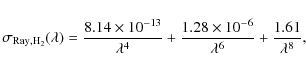 |
(15) |
where
The total Rayleigh scattering optical depth is
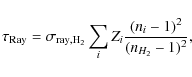 |
(16) |
where Zi is the column density and ni the index of refraction of the ith constituent
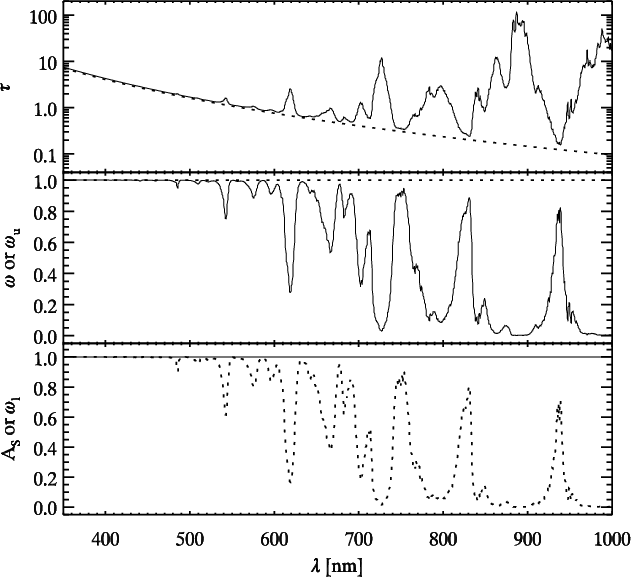 |
Figure 15:
Wavelength dependences of the model parameters total optical depth
|
| Open with DEXTER | |
Because of the strong wavelength dependence of the Rayleigh scattering cross section,
![]() changes significantly from the UV to the near-IR (Fig. 15, top panel). Keeping
changes significantly from the UV to the near-IR (Fig. 15, top panel). Keeping ![]() and
and ![]() fixed (no absorber)
yields the intensity and polarization results given in Figs. 5 and 8 as function of
fixed (no absorber)
yields the intensity and polarization results given in Figs. 5 and 8 as function of
![]() ,
which are in this case equivalent to results as function of
,
which are in this case equivalent to results as function of ![]() .
.
The wavelength dependent single scattering albedo
![]() follows from the CH4
absorption optical depth
follows from the CH4
absorption optical depth
![]() and the Rayleigh scattering optical depth according to
and the Rayleigh scattering optical depth according to
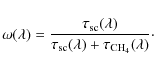 |
(17) |
The absorption cross sections
The intensity
![]() ,
fractional polarization
,
fractional polarization
![]() ,
and polarized intensity
,
and polarized intensity
![]() is determined from the wavelength dependent model parameters for our two cases at quadrature and opposition (Fig. 16).
is determined from the wavelength dependent model parameters for our two cases at quadrature and opposition (Fig. 16).
![\begin{figure}
\par\includegraphics[width=16.9cm,clip]{11760f16.eps}
\end{figure}](/articles/aa/full_html/2009/34/aa11760-09/img206.png) |
Figure 16: Model spectra for the intensity, polarization, and polarized intensity at quadrature ( left) and intensity, radial polarization, and radial polarized intensity at opposition ( right). Lines as in Fig. 15. |
| Open with DEXTER | |
At quadrature both examples show similar results. In both cases the polarization is enhanced and the polarized intensity is reduced within methane absorption bands, only the changes are less pronounced for a non-absorbing upper layer. The polarized intensity
![]() also drops with wavelength, but it is overall higher in the second case because the polarizing Rayleigh scattering extends to deeper layers. The biggest qualitative difference is seen in the continuum polarization
also drops with wavelength, but it is overall higher in the second case because the polarizing Rayleigh scattering extends to deeper layers. The biggest qualitative difference is seen in the continuum polarization
![]() .
In the case of an underlying reflecting cloud,
.
In the case of an underlying reflecting cloud,
![]() drops towards longer wavelengths because of the smaller scattering optical depth above the diffusely scattering cloud. In the second case there is only polarizing Rayleigh scattering and no depolarization effect, so that the increasing absorption with wavelength in the lower layer results in a higher polarization.
drops towards longer wavelengths because of the smaller scattering optical depth above the diffusely scattering cloud. In the second case there is only polarizing Rayleigh scattering and no depolarization effect, so that the increasing absorption with wavelength in the lower layer results in a higher polarization.
Similar spectropolarimetric models but with a Jupiter-like homogeneous atmosphere (higher column density, less methane than in our example) above both a dark surface
![]() and a reflecting extended cloud were discussed by Stam et al. (2004) for
and a reflecting extended cloud were discussed by Stam et al. (2004) for
![]() .
The qualitative behavior of intensity and polarization with wavelength is quite similar to our example. However, for the same column density and methane fraction we find a significantly lower intensity and higher polarization within methane bands. The origin of this discrepancy is unclear. A further comparison with intensity calculations for a Neptune-like atmosphere by Sromosvky (2005a) shows a very good agreement at all wavelengths. Based on this we conclude that our model spectra should be correct.
.
The qualitative behavior of intensity and polarization with wavelength is quite similar to our example. However, for the same column density and methane fraction we find a significantly lower intensity and higher polarization within methane bands. The origin of this discrepancy is unclear. A further comparison with intensity calculations for a Neptune-like atmosphere by Sromosvky (2005a) shows a very good agreement at all wavelengths. Based on this we conclude that our model spectra should be correct.
Intensity and polarized intensity at opposition behave qualitatively similar to the large phase angle case. However the fractional polarization
![]() is completely different. Absorbing particles in the upper layer tend to reduce the fractional limb polarization, while absorption in the lower layer enhances it. Observations of the limb polarization of Uranus and Neptune (Joos & Schmid 2007) show that the fractional polarization is indeed enhanced within methane bands. Clearly for modeling limb polarization of these planets in absorption bands it is important to take into account the proper vertical stratification of the absorbing component. A detailed model accounting for methane saturation and freeze-out to fit the observations is beyond the scope of this paper.
is completely different. Absorbing particles in the upper layer tend to reduce the fractional limb polarization, while absorption in the lower layer enhances it. Observations of the limb polarization of Uranus and Neptune (Joos & Schmid 2007) show that the fractional polarization is indeed enhanced within methane bands. Clearly for modeling limb polarization of these planets in absorption bands it is important to take into account the proper vertical stratification of the absorbing component. A detailed model accounting for methane saturation and freeze-out to fit the observations is beyond the scope of this paper.
6 Special cases and diagnostic diagrams
We explore some special and extreme model cases in diagnostic diagrams of observational parameters for phase angle
6.1 Fractional polarization versus intensity
Figure 17 displays the diagnostic diagram for
the reflectivity
![]() and the relative polarization
and the relative polarization
![]() at phase angle
at phase angle
![]() .
Also indicated are the iso-contours for the
polarization flux
.
Also indicated are the iso-contours for the
polarization flux
![]() .
.
The diagram shows points for special model cases and curves for the dependence on specific model parameters. The shaded area defines the area of observational parameters covered by our 3-parameter model grid for Rayleigh scattering (Sect. 3). Including isotropic scattering (Sect. 4.1) or having a vertically inhomogeneous atmosphere (Sect. 4.3) does not expand the covered area.
![\begin{figure}
\par\includegraphics[width=8.5cm,clip]{11760f17.eps}
\end{figure}](/articles/aa/full_html/2009/34/aa11760-09/img208.png) |
Figure 17:
Intensity vs. polarization at quadrature for the
grid models. The shaded area indicates the possible range for Rayleigh and isotropic models. The symbols and lines indicate:
semi-infinite conservative Rayleigh scattering (square), Lambert
sphere (round), and black planet (diamond). The
dash-dotted line shows semi-infinite models, the dashed
and full line finite models without absorption ( |
| Open with DEXTER | |
Figure 17 emphasizes that it is not possible to have a Rayleigh scattering planet with both very high albedo and polarization. A high albedo implies either a lot of multiple or isotropic scattering, which both reduce the fractional polarization. On the other hand a high polarization implies mainly single scattering and therefore strong absorption and a low reflectivity. The maximal polarization at a fixed intensity is given by the model with a conservative
![]() scattering layer over a dark (
scattering layer over a dark (
![]() )
surface and appropriate
)
surface and appropriate
![]() .
The semi-infinite atmosphere with varying
.
The semi-infinite atmosphere with varying ![]() gives only slightly lower results than the former models. The maximum of the product
gives only slightly lower results than the former models. The maximum of the product
![]() is reached for the conservative semi-infinite atmosphere (
is reached for the conservative semi-infinite atmosphere (
![]() ). Since the polarized intensity Q is independent of the surface albedo
). Since the polarized intensity Q is independent of the surface albedo ![]() ,
a change in
,
a change in ![]() is equivalent to a shift along the Q iso-contours in the diagram.
is equivalent to a shift along the Q iso-contours in the diagram.
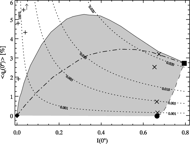 |
Figure 18: Geometric albedo vs. disk-integrated radial polarization at opposition for the grid models. The models are the same as in Fig. 17. |
| Open with DEXTER | |
The diagram also indicates the location of the haze models discussed in Sect. 4.2. Most of the haze models lie within the same area as Rayleigh scattering. Only for very thick haze layers with high single-scattering albedo is it theoretically possible to get somewhat higher fractional polarization for a given intensity.
Figure 18 is the same diagram at opposition
for the geometric albedo
![]() ,
the disk-integrated limb polarization
,
the disk-integrated limb polarization
![]() and iso-contours for the radial polarized intensity
and iso-contours for the radial polarized intensity
![]() .
Like for large phase angles, the limb polarization for fixed intensity is highest for the conservative Rayleigh scattering layers over a dark surface. However, for
.
Like for large phase angles, the limb polarization for fixed intensity is highest for the conservative Rayleigh scattering layers over a dark surface. However, for
![]() the polarization drops to 0%, while at large phase angles with
the polarization drops to 0%, while at large phase angles with
![]() it raises towards 100% when the few reflected photons are mainly singly scattered. The semi-infinite models provide a distinctly lower fractional polarization signal than a finite conservatively scattering atmosphere over a dark surface. The fractional limb polarization for very low albedos can be significantly higher for atmospheres with haze than for Rayleigh scattering, because the unpolarized backscattering is greatly reduced.
it raises towards 100% when the few reflected photons are mainly singly scattered. The semi-infinite models provide a distinctly lower fractional polarization signal than a finite conservatively scattering atmosphere over a dark surface. The fractional limb polarization for very low albedos can be significantly higher for atmospheres with haze than for Rayleigh scattering, because the unpolarized backscattering is greatly reduced.
For models with two polarizing layers with different absorption properties, the results are located in the same area as for one layer above a surface. The limiting cases are models with a completely dark lower layer (equivalent to a dark surface), and two identical layers (equivalent to a single semi-infinite layer). For atmospheres that contain also isotropically scattering particles the polarization is always lower and the intensity either slightly enhanced or reduced depending on ![]() because of the different scattering phase functions.
because of the different scattering phase functions.
![\begin{figure}
\par\includegraphics[width=8.5cm,clip]{11760f19.eps}
\end{figure}](/articles/aa/full_html/2009/34/aa11760-09/img212.png) |
Figure 19: Disk-integrated radial polarization at opposition vs. polarization at quadrature for the grid. The models are the same as in Fig. 17. All Rayleigh scattering models lie in the dark shaded area, (partly) isotropic models also in the light shaded area. |
| Open with DEXTER | |
6.2 Polarization near
versus limb polarization
For the prediction or the future interpretation of the polarization of extrasolar planets it is of interest to compare the polarization at phase angles near quadrature with the limb polarization at opposition.
Figure 19 shows a diagram for the fractional
polarization
![]() and the fractional limb
polarization
and the fractional limb
polarization
![]() .
Again the special models
are indicated with black symbols and lines as in
Figs. 17 and 18.
.
Again the special models
are indicated with black symbols and lines as in
Figs. 17 and 18.
A lower limit for the polarization fraction at phase angles
![]() can be set from the limb polarization at opposition
can be set from the limb polarization at opposition
![]() for Rayleigh scattering or partly isotropic scattering atmospheres. For example a limb polarization of
for Rayleigh scattering or partly isotropic scattering atmospheres. For example a limb polarization of
![]() %
implies a minimal polarization of
%
implies a minimal polarization of
![]() %.
The upper limit for the polarization fraction
%.
The upper limit for the polarization fraction
![]() )
is not
well constrained by
)
is not
well constrained by
![]() .
The lower limit for Rayleigh or isotropic scattering may
overestimate the polarization at large phase angles only for very thick and bright haze layers.
.
The lower limit for Rayleigh or isotropic scattering may
overestimate the polarization at large phase angles only for very thick and bright haze layers.
A tighter correlation is obtained for the polarization flux
![]() and the limb polarization flux
and the limb polarization flux
![]() ,
which is shown in Fig. 20. All Rayleigh scattering models are located
in a narrow area along a line from the origin (Lambert sphere / black planet) to the semi-infinite, conservative Rayleigh scattering model. Thus, for Rayleigh scattering atmospheres, one can predict the large phase angle polarization flux
,
which is shown in Fig. 20. All Rayleigh scattering models are located
in a narrow area along a line from the origin (Lambert sphere / black planet) to the semi-infinite, conservative Rayleigh scattering model. Thus, for Rayleigh scattering atmospheres, one can predict the large phase angle polarization flux ![]() from the limb polarization flux
from the limb polarization flux
![]() and vice versa. The area is slightly broadened if isotropic scattering is included in the models, but the relation still holds quite well. Only very thick and high albedo haze layers show a significantly lower
and vice versa. The area is slightly broadened if isotropic scattering is included in the models, but the relation still holds quite well. Only very thick and high albedo haze layers show a significantly lower
![]() )
for a given
)
for a given
![]() .
.
6.3 Broadband polarized intensity
Color indices of observational parameters are often relatively easy to measure and they are helpful for the characterization of atmospheres. From the atmosphere models they are obtained by averaging spectral results (Sect. 5) over the filter bandwidths.
![\begin{figure}
\par\includegraphics[width=8.5cm,clip]{11760f20.eps}
\end{figure}](/articles/aa/full_html/2009/34/aa11760-09/img218.png) |
Figure 20: Disk-integrated radial polarized flux at opposition vs. polarized flux at quadrature for the grid models. The indicated models are the same as in Fig. 17. All Rayleigh scattering models lie in the dark shaded area, (partly) isotropic models also in the light shaded area. |
| Open with DEXTER | |
Here we discuss the colors for a Rayleigh scattering atmosphere with methane as a main absorber. It is investigated how the polarized intensity color changes as a function of methane mixing ratio and column density above a cloud or surface. Color indices are calculated by integrating
![]() over the wavelength range foreseen for filters in the SPHERE/ZIMPOL instrument (Beuzit et al. 2006). The filters are assumed to have flat transmission curves with cut offs at 555 and 700 nm (R-band) and 715 and 865 nm (I-band). We concentrate on the color index of the polarized intensity
QI/QR (Fig. 21).
over the wavelength range foreseen for filters in the SPHERE/ZIMPOL instrument (Beuzit et al. 2006). The filters are assumed to have flat transmission curves with cut offs at 555 and 700 nm (R-band) and 715 and 865 nm (I-band). We concentrate on the color index of the polarized intensity
QI/QR (Fig. 21).
The polarized intensity is higher at shorter wavelengths, and QI/QR < 1 for all models because of the decrease of the Rayleigh scattering cross section with wavelength and the general increase of the absorption cross section of methane with wavelength. QI/QR is near 1 only for very thick atmospheres with very little methane or very thin atmospheres above a surface with wavelength independent scattering properties. In the former case QR and QI are very high, in the latter very low. For intermediately thick atmospheres the color index QI/QR mainly depends on the methane mixing ratio, while QR mainly depends on the column density.
From this diagram we may predict that a color index of
![]() could be typical for Rayleigh scattering atmospheres with methane absorption. Aerosol particles and absorbers other than methane are expected to have a different spectral dependence of the scattering and absorption cross sections.
could be typical for Rayleigh scattering atmospheres with methane absorption. Aerosol particles and absorbers other than methane are expected to have a different spectral dependence of the scattering and absorption cross sections.
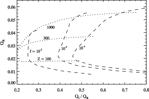 |
Figure 21:
Polarized intensity QR as a function of color
QI/QR where QR is the broad-band R signal (555 to 700 nm) and QI the broad-band I signal (715 to 865 nm) for Rayleigh scattering planets with methane at 90 |
| Open with DEXTER | |
7 Conclusions
This paper presents a grid of model results for the intensity and polarization of
Rayleigh scattering planetary atmospheres, covering the model parameter space in a systematic
way. The model parameters considered are the single scattering albedo
![]() ,
which describes absorption, the
scattering optical depth of the layer
,
which describes absorption, the
scattering optical depth of the layer
![]() ,
and the albedo
of a Lambert surface
,
and the albedo
of a Lambert surface ![]() .
The results of these model calculations
are available in electronic form at CDS (see Appendix A).
In addition we explore models which
combine Rayleigh and isotropic scattering, as well as particles with
strong forward scattering and atmospheres with vertical stratification.
.
The results of these model calculations
are available in electronic form at CDS (see Appendix A).
In addition we explore models which
combine Rayleigh and isotropic scattering, as well as particles with
strong forward scattering and atmospheres with vertical stratification.
Simple Rayleigh scattering models are a good first approximation to the polarization of light reflected from planetary atmospheres because some amount of Rayleigh-like scattering by molecules or very small aerosol particles can be expected in any atmosphere. From the model grid, which basically provides monochromatic results, the spectropolarimetric signal can be calculated. This is done by considering the wavelength dependence of Rayleigh scattering and absorption in an atmosphere with given column density and particle abundance (see Sect. 5).
The phase curves for the reflected intensity and polarization show a strong dependence on phase but they always have similar shapes (see Fig. 2). However, the absolute level of the phase curve is a strong function of atmospheric parameters such as the abundance of absorbers or aerosol particles, the optical thickness of the Rayleigh scattering layer, or the albedo of the surface layer underneath (Sect. 3 and 4, see also Kattwar & Adams 1971).
The model calculations demonstrate that polarimetric observations
would provide strong constraints on the atmospheric properties of the
planetary atmospheres. An example is the polarization flux ![]() of the reflected light which for optically thick atmospheres is a
simple function of the single scattering albedo roughly according to
of the reflected light which for optically thick atmospheres is a
simple function of the single scattering albedo roughly according to
![]()
![]() .
If both polarization and
intensity can be measured, then one can distinguish between highly
reflective and absorbing planets with or without substantial layers of
Rayleigh-like scattering particles.
.
If both polarization and
intensity can be measured, then one can distinguish between highly
reflective and absorbing planets with or without substantial layers of
Rayleigh-like scattering particles.
According to the models a similar diagnostic is possible with observations of the geometric albedo, center-to-limb polarization profile, and limb polarization for solar system planets near opposition. The limb polarization is in addition particularly sensitive to the vertical stratification of scattering or absorbing particles located high in the atmosphere.
Table A.1: Extract of model grid results.
The diagnostic potential is further enhanced if data for different spectral features, e.g. inside and outside of absorption bands, or from different spectral wavelength regions can be combined (Sect. 5, see also Stam et al. 2004).
The calculations presented in this work are based on simple atmosphere models and they are therefore mainly useful for a first interpretation of data. For spectropolarimetric data of high quality, which are already available for solar system planets, one should use more sophisticated atmospheric models including a more detailed geometric structure, accurate abundances, and better scattering models for aerosol particles. With such models it might be possible for polarimetric studies to make a contribution to our knowledge on the rather well known atmospheres of solar system objects.
Nonetheless the simple limb polarization models are of interest because they link the model results for large phase angles, suitable for extrasolar planet research, to models which can be easily compared with observations of solar system objects. Thus it may be possible to associate polarimetric observations of extrasolar planets to solar system objects. On the other hand it is possible to predict the expected polarization for quadrature phase of Uranus- and Neptune-like extrasolar planets with this simple model grid based on the existing limb polarization measurements of Uranus and Neptune (Fig. 20).
Polarimetric measurements for extrasolar planets are expected in the
near future from high precision polarimeters. The measurements will first
provide the polarimetric contrast, which is the ratio of
the polarization flux from the planet ![]() to the flux of the central star
according to
to the flux of the central star
according to
 |
(18) |
where R is the radius of the planet and D the distance from its central star.
Very sensitive polarimetric measurements of stars with known
close-in planets already exist, taken e.g. with the PLANETPOL instrument
(Hough et al. 2006; Lucas et al. 2009). This instrument
measures the polarized intensity ![]() of the planet diluted by the
unpolarized flux of the central star. It is then difficult to
separate the fractional polarization q and the reflected intensity
I. D is known from the radial velocity curve, but already the
radius of the planet R may be hard to derive if the system shows no
transits. For photometrically very stable stars the reflected
intensity
of the planet diluted by the
unpolarized flux of the central star. It is then difficult to
separate the fractional polarization q and the reflected intensity
I. D is known from the radial velocity curve, but already the
radius of the planet R may be hard to derive if the system shows no
transits. For photometrically very stable stars the reflected
intensity
![]() may be measurable with photometry of the phase
curve with high precision instruments like MOST (e.g. Rowe et al. 2008).
An uncertainty in the planet radius will affect the precision of the
estimation of the normalized reflected intensity
may be measurable with photometry of the phase
curve with high precision instruments like MOST (e.g. Rowe et al. 2008).
An uncertainty in the planet radius will affect the precision of the
estimation of the normalized reflected intensity ![]() (or reflectivity) of the planet.
(or reflectivity) of the planet.
SPHERE, the future ``VLT planet finder'', which includes the
high precision imaging polarimeter ZIMPOL, could provide
successful polarimetric detections (Beuzit et al. 2006; Schmid et al. 2006b). This
instrument will be able to spatially resolve nearby (d < 10 pc) star-planet systems and allow a polarimetric search for faint companions to stars.
In a first step only the differential polarization signal,
i.e. the polarization flux ![]() ,
can be measured in the
residual halo of the central star. The measurement of the intensity
signal
,
can be measured in the
residual halo of the central star. The measurement of the intensity
signal ![]() might be possible if further progress in
techniques like angular differential imaging is achieved. Even if
a determination of
might be possible if further progress in
techniques like angular differential imaging is achieved. Even if
a determination of
![]() is possible, an
uncertainty remains in the translation to normalized intensity
is possible, an
uncertainty remains in the translation to normalized intensity
![]() if the radius of the planet is not known.
if the radius of the planet is not known.
Thus it may initially be quite difficult to measure intensity and radius. For this reason it is important to investigate the diagnostic potential of the wavelength dependence in the polarization flux in more detail. For example the R-band and I-band yield a polarization color index QI/QR from which it should be possible to infer constraints on the Rayleigh scattering optical depth or the strength of absorption bands (see Sect. 6.3). Another route of investigation for atmospheres of extrasolar planets are measurements of the phase dependence of the polarization flux. For example the location of the maximum of Q along the phase curve is sensitive to the presence of aerosol particles, as discussed in Sect. 4.2. For planets in eccentric orbits the dependence of the polarization flux on the separation from the host star can be determined.
One can hope that the current rapid progress in extrasolar planet observations continues, so that intensity measurements and accurate radius estimates for extrasolar planets become available soon after the first polarization flux detections, using the next generation of ground based telescopes and space instruments. Such instruments, if equipped with a polarimetric observing mode, would allow a broad range of observational programs on the reflected intensity and polarization from planets.
Acknowledgements
This work is supported by the Swiss National Science Foundation (SNSF). We thank Harry Nussbaumer and Franco Joos for carefully reading the manuscript.
Appendix A: Model grid tables
Our extensive model grid of intensity and polarization phase curves for homogeneous Rayleigh scattering atmospheres (Sect. 3) is available in electronic form at CDS. Table A.1 shows a sample of the first few lines and columns. The table is structured as follows: Model parameters: Column 1: scattering optical thickness
![]() ,
Column 2: single scattering albedo
,
Column 2: single scattering albedo ![]() ,
Column 3: surface albedo
,
Column 3: surface albedo ![]() ,
Model results: Column 4: spherical albedo
,
Model results: Column 4: spherical albedo
![]() ,
Column 5: geometric albedo
,
Column 5: geometric albedo
![]() ,
Column 6: limb polarization flux
,
Column 6: limb polarization flux
![]() ,
Column 7:
,
Column 7:
![]() ,
Column 8:
,
Column 8:
![]() ,..., Column 40:
,..., Column 40:
![]() Column 41:
Column 41:
![]() ,..., Column 74:
,..., Column 74:
![]() .
Columns 7 to 74 are
.
Columns 7 to 74 are ![]() and
and ![]() spaced in 5 degree intervals.
spaced in 5 degree intervals.
![]() is equivalent to
is equivalent to
![]() in our calculations.
in our calculations.
![]() ,
,
![]() and
and
![]() are very close to zero for all models and are not listed.
are very close to zero for all models and are not listed.
All results are disk-integrated. Binning, normalization and errors are described in Sect. 2.4. For all calculations the number of photons was chosen such that
![]() % for phase angles
% for phase angles
![]() ,
and therefore
,
and therefore
![]() %.
%.
The model grid spans the following parameters:
![]() ,
10, 5, 2, 1, 0.8, 0.6, 0.4, 0.3, 0.2, 0.1, 0.05, 0.01,
,
10, 5, 2, 1, 0.8, 0.6, 0.4, 0.3, 0.2, 0.1, 0.05, 0.01,
![]() ,
0.99, 0.95, 0.9, 0.8, 0.6, 0.4, 0.2, 0.1,
,
0.99, 0.95, 0.9, 0.8, 0.6, 0.4, 0.2, 0.1,
![]() ,
0.3, 0. Models for only three values of
,
0.3, 0. Models for only three values of ![]() are given because the polarized intensity is independent of
are given because the polarized intensity is independent of ![]() and the intensity drops nearly linearly with increasing
and the intensity drops nearly linearly with increasing ![]() .
Models with
.
Models with
![]() were calculated only for
were calculated only for
![]() since the results are independent of
since the results are independent of ![]() .
Instead of a model with
.
Instead of a model with
![]() and
and
![]() ,
we calculated the model with
,
we calculated the model with
![]() to reduce computation time, but the results are equivalent.
to reduce computation time, but the results are equivalent.
The spherical albedo
![]() in Col. 4 is the ratio of reflected photons in any direction to total incoming photons, while the geometric albedo
in Col. 4 is the ratio of reflected photons in any direction to total incoming photons, while the geometric albedo
![]() in column 5 is the disk-integrated reflected intensity at opposition normalized to the reflection of a white Lambertian disk. For our sample of Rayleigh scattering models, typically
in column 5 is the disk-integrated reflected intensity at opposition normalized to the reflection of a white Lambertian disk. For our sample of Rayleigh scattering models, typically
![]() .
.
References
- Abhyankar, K. D., & Fymat, A. L. 1970, A&A, 4, 101 [NASA ADS] (In the text)
- Abhyankar, K. D., & Fymat, A. L. 1971, ApJS, 23, 35 [NASA ADS] [CrossRef] (In the text)
- Bailey, J. 2007, Astrobiology, 7, 320 [NASA ADS] [CrossRef] (In the text)
- Baines, K. H., & Bergstralh, J. T. 1986, Icarus, 65, 406 [NASA ADS] [CrossRef] (In the text)
- Beuzit, J.-L., Feldt, M., Dohlen, K., et al. 2006, Msngr, 125, 29 [NASA ADS] (In the text)
- Bhatia, R. K., & Abhyankar, K. D. 1982, JApA, 3, 303 [NASA ADS] (In the text)
- Braak, C. J., de Haan, J. F., van der Mee, J. W., Hovenier, J. W., & Travis, L. D. 2001, JQSRT, 69, 585 [NASA ADS]
- Braak, C. J., de Haan, J. F., Hovenier, J. W., & Travis, L. D. 2002, Icarus, 157, 401 [NASA ADS] [CrossRef] (In the text)
- Cashwell, E. D., & Everett, D. J. 1959, A practical manual on the Monte Carlo method for random walk problems (London: Pergamon Press) (In the text)
- Chandrasekhar, S. 1950, Radiative Transfer (Oxford: Clarendon Press) (In the text)
- Code, A. D., & Whitney, B. A. 1995, ApJ, 441, 400 [NASA ADS] [CrossRef] (In the text)
- Coffeen, D. L., & Gehrels, T. 1969, AJ, 74, 433 [NASA ADS] [CrossRef] (In the text)
- Coulson, K. L., Dave, J. V., & Sekera, Z. 1960, Tables Related to Radiation Emerging from a Planetary Atmosphere with Rayleigh Scattering (Berkeley: Univ. of California Press) (In the text)
- Dalgarno, A., & Williams, D. A. 1962, ApJ, 136, 690 [NASA ADS] [CrossRef] (In the text)
- Dlugach, J. M., & Yanovitskij, E. G. 1974, Icarus, 22, 66 [NASA ADS] [CrossRef] (In the text)
- Dollfus, A., & Coffeen, D. L. 1970, A&A, 8, 251 [NASA ADS] (In the text)
- Hansen, J. E., & Hovenier, J. W. 1974, J. Atmos. Sciences, 31, 1137 [NASA ADS] [CrossRef] (In the text)
- Horak, H. G. 1950, ApJ, 112, 445 [NASA ADS] [CrossRef]
- Hough, J. H., Lucas, P. W., Bailey, J. A., et al. 2006, PASP, 118, 1302 [NASA ADS] [CrossRef] (In the text)
- Joos, F., & Schmid, H. M. 2007, A&A, 463, 1201 [NASA ADS] [CrossRef] [EDP Sciences] (In the text)
- Karkoschka, E. 1994, Icarus, 111, 174 [NASA ADS] [CrossRef] (In the text)
- Karkoschka, E. 2001, Icarus, 151, 84 [NASA ADS] [CrossRef] (In the text)
- Kattawar, G. W., & Adams, C. N. 1971, ApJ, 167, 183 [NASA ADS] [CrossRef] (In the text)
- Leinert, C., Richter, I., Pitz, E., & Planck, B. 1981, A&A, 103, 177 [NASA ADS] (In the text)
- Levasseur-Regourd A. C., Hadamcik, E., & Renard, J. B. 1996, A&A, 313, 327 [NASA ADS] (In the text)
- Lucas, P. W., Hough, J. H., Bailey, et al. 2009, MNRAS, 393, 229 [NASA ADS] [CrossRef] (In the text)
- Lyot, B. 1929, Ann. Observ. Meudon, 8 (In the text)
- Prather, M. J. 1974, ApJ, 192, 787 [NASA ADS] [CrossRef] (In the text)
- Price, M. 1978, Icarus, 35, 93 [NASA ADS] [CrossRef] (In the text)
- Rowe, J. F., Matthews, J. M., Seager, S., et al. 2008, ApJ, 689, 1345 [NASA ADS] [CrossRef] (In the text)
- Seager, S., Whitney, B. A., & Sasselov, D. D. 2000, ApJ, 540, 504 [NASA ADS] [CrossRef] (In the text)
- Schmid, H. M. 1992, A&A, 254, 224 [NASA ADS] (In the text)
- Schmid, H. M., Joos, F., & Tschan, D. 2006a, A&A, 254, 224 (In the text)
- Schmid, H. M., Beuzit, J.-L., Feldt, M., et al. 2006b, in Direct Imaging of Exoplanets: Science and Techniques, ed. C. Aime, & F. Vakili (Cambridge: Cambridge Univ. Press), IAU Colloq., 200, 165 (In the text)
- Smith P. H., & Tomasko M. G. 1984, Icarus, 58, 35 [NASA ADS] [CrossRef] (In the text)
- Sromovsky, L. A. 2005a, Icarus, 173, 254 [NASA ADS] [CrossRef] (In the text)
- Sromovsky, L. A. 2005b, Icarus, 173, 284 [NASA ADS] [CrossRef] (In the text)
- Sromovsky, L. A., & Fry, P. M. 2007, Icarus, 192, 527 [NASA ADS] [CrossRef] (In the text)
- Stam, D. M. 2008, A&A, 482, 989 [NASA ADS] [CrossRef] [EDP Sciences] (In the text)
- Stam, D. M., Hovenier, J. W., Waters, L. B. F. M. 2004, A&A, 428, 663 [NASA ADS] [CrossRef] [EDP Sciences] (In the text)
- Stam, D. M., de Rooij, W. A., Cornet, G., & Hovenier, J. W. 2006, A&A, 452, 669 [NASA ADS] [CrossRef] [EDP Sciences] (In the text)
- Tomasko, M. G., & Doose, L. R. 1984, Icarus, 58, 1 [NASA ADS] [CrossRef] (In the text)
- Tomasko, M. G., & Smith, P. H. 1982, Icarus, 51, 65 [NASA ADS] [CrossRef] (In the text)
- Tomasko, M. G., Doose, L., Engle, S., et al. 2008, Planetary and Space Science, 56, 669 [NASA ADS] [CrossRef] (In the text)
- Trafton, L. 1976, ApJ, 207, 1007 [NASA ADS] [CrossRef] (In the text)
- van de Hulst, H. C. 1980, Multiple Light Scattering, 2nd Volume (New York: Academic Press) (In the text)
- West, R. A. 1991, Appl. Opt., 36, 5316 [NASA ADS] [CrossRef] (In the text)
- West, R. A., Hart, H., Simmons, K. E., et al. 1983, J. Geophys. Res., 88, 8699 [NASA ADS] [CrossRef]
- Wiktorowicz, S. J. 2009, ApJ, 696, 1116 [NASA ADS] [CrossRef] (In the text)
- Witt, A. N. 1977, ApJS, 35, 1 [NASA ADS] [CrossRef] (In the text)
- Wolf, S., Henning Th., & Stecklum, B. 1999, A&A, 349, 839 [NASA ADS] (In the text)
Footnotes
- ... atmospheres
- Full Table A.1 is only available in electronic form at the CDS via anonymous ftp to cdsarc.u-strasbg.fr (130.79.128.5) or via http://cdsweb.u-strasbg.fr/cgi-bin/qcat?J/A+A/504/259
- ... constituent
-
 ,
,
 ,
,
 .
.
- ... km-am.
- 1 km-am =
 molecules cm-2.
All Tables
Table 1:
Reflectivity ![]() ,
polarization fraction
,
polarization fraction ![]() and polarized intensity
and polarized intensity ![]() phase curves for a very deep
(
phase curves for a very deep
(![]() )
conservative
)
conservative
![]() Rayleigh scattering atmosphere above a perfectly
reflecting Lambert surface (surface albedo
Rayleigh scattering atmosphere above a perfectly
reflecting Lambert surface (surface albedo
![]() ).
).
Table 2:
Best fit parameter
![]() for the parametrization of the polarized intensity Q (Eq. (5)).
for the parametrization of the polarized intensity Q (Eq. (5)).
Table A.1: Extract of model grid results.
All Figures
| |
Figure 1: Model geometry. The dashed line represents the trajectory of a reflected photon. |
| Open with DEXTER | |
| In the text | |
| |
Figure 2:
Left: phase dependence of the intensity I, fractional
polarization q and polarized intensity Q for Rayleigh
scattering atmospheres. Right: radial dependence of the intensity I, radial
polarization qr and radial polarized intensity Qr at
opposition. Line styles denote: semi-infinite case
|
| Open with DEXTER | |
| In the text | |
| |
Figure 3:
Radial intensity curves for different model parameters normalized to the central disk intensity, showing examples of limb darkening and limb brightening. The solid line is the calculated model and the dotted line the best fit with the Minnaert law. (a), (b) and (c) are for conservatively ( |
| Open with DEXTER | |
| In the text | |
| |
Figure 4:
Intensity, polarization and polarized intensity at quadrature as function of single scattering albedo |
| Open with DEXTER | |
| In the text | |
| |
Figure 5:
Intensity, polarization and polarized intensity at quadrature as function of optical depth
|
| Open with DEXTER | |
| In the text | |
| |
Figure 6:
Intensity, polarization and polarized intensity at quadrature as function of surface albedo |
| Open with DEXTER | |
| In the text | |
| |
Figure 7:
Geometric albedo, disk-integrated radial polarization and polarized intensity at opposition as function of single scattering albedo |
| Open with DEXTER | |
| In the text | |
| |
Figure 8:
Geometric albedo, disk-integrated radial polarization and polarized intensity at opposition as function of optical depth
|
| Open with DEXTER | |
| In the text | |
| |
Figure 9:
Geometric albedo, disk-integrated radial polarization and polarized intensity at opposition as function of surface albedo |
| Open with DEXTER | |
| In the text | |
| |
Figure 10:
Polarization of atmospheres with Rayleigh and isotropic scattering at 90 |
| Open with DEXTER | |
| In the text | |
| |
Figure 11:
Probability density function
|
| Open with DEXTER | |
| In the text | |
| |
Figure 12:
Phase dependence of the intensity I, fractional
polarization q and polarized intensity Q for a haze layer. Left: semi-infinite case
|
| Open with DEXTER | |
| In the text | |
| |
Figure 13:
Radial dependence of the intensity I, radial
polarization qr and radial polarized intensity Qr at
opposition for a haze layer. Left: semi-infinite case
|
| Open with DEXTER | |
| In the text | |
| |
Figure 14:
Fractional polarization q as function of
|
| Open with DEXTER | |
| In the text | |
| |
Figure 15:
Wavelength dependences of the model parameters total optical depth
|
| Open with DEXTER | |
| In the text | |
| |
Figure 16: Model spectra for the intensity, polarization, and polarized intensity at quadrature ( left) and intensity, radial polarization, and radial polarized intensity at opposition ( right). Lines as in Fig. 15. |
| Open with DEXTER | |
| In the text | |
| |
Figure 17:
Intensity vs. polarization at quadrature for the
grid models. The shaded area indicates the possible range for Rayleigh and isotropic models. The symbols and lines indicate:
semi-infinite conservative Rayleigh scattering (square), Lambert
sphere (round), and black planet (diamond). The
dash-dotted line shows semi-infinite models, the dashed
and full line finite models without absorption ( |
| Open with DEXTER | |
| In the text | |
| |
Figure 18: Geometric albedo vs. disk-integrated radial polarization at opposition for the grid models. The models are the same as in Fig. 17. |
| Open with DEXTER | |
| In the text | |
| |
Figure 19: Disk-integrated radial polarization at opposition vs. polarization at quadrature for the grid. The models are the same as in Fig. 17. All Rayleigh scattering models lie in the dark shaded area, (partly) isotropic models also in the light shaded area. |
| Open with DEXTER | |
| In the text | |
| |
Figure 20: Disk-integrated radial polarized flux at opposition vs. polarized flux at quadrature for the grid models. The indicated models are the same as in Fig. 17. All Rayleigh scattering models lie in the dark shaded area, (partly) isotropic models also in the light shaded area. |
| Open with DEXTER | |
| In the text | |
| |
Figure 21:
Polarized intensity QR as a function of color
QI/QR where QR is the broad-band R signal (555 to 700 nm) and QI the broad-band I signal (715 to 865 nm) for Rayleigh scattering planets with methane at 90 |
| Open with DEXTER | |
| In the text | |
Copyright ESO 2009
Current usage metrics show cumulative count of Article Views (full-text article views including HTML views, PDF and ePub downloads, according to the available data) and Abstracts Views on Vision4Press platform.
Data correspond to usage on the plateform after 2015. The current usage metrics is available 48-96 hours after online publication and is updated daily on week days.
Initial download of the metrics may take a while.