| Issue |
A&A
Volume 504, Number 1, September II 2009
|
|
|---|---|---|
| Page(s) | 239 - 248 | |
| Section | The Sun | |
| DOI | https://doi.org/10.1051/0004-6361/200811445 | |
| Published online | 09 July 2009 | |
Hydrogen Lyman- and Lyman-
 spectral radiance profiles in the quiet Sun
H. Tian1,2 - W. Curdt1 - E. Marsch1 - U. Schühle1
1 - Max-Planck-Institut für Sonnensystemforschung,
Max-Planck-Str. 2, 37191 Katlenburg-Lindau, Germany
2 - School of Earth and Space Sciences, Peking University, PR China
Received 28 November 2008 / Accepted 29 June 2009
Abstract
Aims. We extend earlier work by studying the line profiles of the hydrogen Lyman-![]() and Lyman-
and Lyman-![]() lines in the quiet Sun. They were obtained quasi-simultaneously in a raster scan with a size of about 150
lines in the quiet Sun. They were obtained quasi-simultaneously in a raster scan with a size of about 150
![]()
![]() 120
120
![]() near disk center.
near disk center.
Methods. The self-reversal depths of the Ly-![]() and Ly-
and Ly-![]() profiles. we are quantified by measuring the maximum spectral radiances of the two horns and the minimum spectral radiance of the central reversal. The information on the asymmetries of the Ly-
profiles. we are quantified by measuring the maximum spectral radiances of the two horns and the minimum spectral radiance of the central reversal. The information on the asymmetries of the Ly-![]() and Ly-
and Ly-![]() profiles is obtained through calculating the 1st and 3rd-order moments of the line profiles. By comparing maps of self-reversal depths and the moments with radiance images of the Lyman lines, photospheric magnetograms, and Dopplergrams of two other optically thin lines, we studied the spatial distribution of the Ly-
profiles is obtained through calculating the 1st and 3rd-order moments of the line profiles. By comparing maps of self-reversal depths and the moments with radiance images of the Lyman lines, photospheric magnetograms, and Dopplergrams of two other optically thin lines, we studied the spatial distribution of the Ly-![]() and Ly-
and Ly-![]() profiles with different self-reversal depths, and investigated the relationship between profile asymmetries and flows in the solar atmosphere.
profiles with different self-reversal depths, and investigated the relationship between profile asymmetries and flows in the solar atmosphere.
Results. We find that the emissions of the Lyman lines tend to be more strongly absorbed in the internetwork, as compared to those in the network region. Almost all of the Ly-![]() profiles are self-reversed, while about 17% of the Ly-
profiles are self-reversed, while about 17% of the Ly-![]() profiles are not reversed. The ratio of Ly-
profiles are not reversed. The ratio of Ly-![]() and Ly-
and Ly-![]() intensities seems to be independent of the magnetic field strength. Most Ly-
intensities seems to be independent of the magnetic field strength. Most Ly-![]() profiles are stronger in the blue horn, whereas most Ly-
profiles are stronger in the blue horn, whereas most Ly-![]() profiles are stronger in the red horn. However, the opposite asymmetries of Ly-
profiles are stronger in the red horn. However, the opposite asymmetries of Ly-![]() and Ly-
and Ly-![]() are not correlated pixel-to-pixel. We also confirm that when larger transition-region downflows are present, the Ly-
are not correlated pixel-to-pixel. We also confirm that when larger transition-region downflows are present, the Ly-![]() and Ly-
and Ly-![]() profiles are more enhanced in the blue and red horns, respectively. The first-order moment of Ly-
profiles are more enhanced in the blue and red horns, respectively. The first-order moment of Ly-![]() ,
which reflects the combined effects of the profile asymmetry and motion of the emitting material, strongly correlates with the Doppler shifts of the Si III and O VI lines, while this correlation is much weaker for Ly-
,
which reflects the combined effects of the profile asymmetry and motion of the emitting material, strongly correlates with the Doppler shifts of the Si III and O VI lines, while this correlation is much weaker for Ly-![]() .
Our analysis shows that both Ly-
.
Our analysis shows that both Ly-![]() and Ly-
and Ly-![]() might be more redshifted if stronger transition-region downflows are present. We also find that the observed average Ly-
might be more redshifted if stronger transition-region downflows are present. We also find that the observed average Ly-![]() profile is redshifted with respect to its rest position.
profile is redshifted with respect to its rest position.
Key words: Sun: UV radiation - Sun: transition region - line: formation - line: profiles
1 Introduction
Hydrogen is the most abundant element in the solar atmosphere. And
thus its resonance lines, especially the Lyman-alpha (Ly-![]() )
and
Lyman-beta (Ly-
)
and
Lyman-beta (Ly-![]() )
lines, play an important role in the overall
radiative energy transport of the Sun (Fontenla et al. 1988).
)
lines, play an important role in the overall
radiative energy transport of the Sun (Fontenla et al. 1988).
Ly-![]() is by far the strongest line in the vacuum ultraviolet (VUV)
spectral range. It is so dominant that
is by far the strongest line in the vacuum ultraviolet (VUV)
spectral range. It is so dominant that ![]() 75% of the
integrated radiance from 800 Å to 1500 Å in the quiet Sun
come from this single line (Wilhelm et al. 1998). Energy losses through
the Ly-
75% of the
integrated radiance from 800 Å to 1500 Å in the quiet Sun
come from this single line (Wilhelm et al. 1998). Energy losses through
the Ly-![]() emission are the most important radiative losses in the
lower transition region, where the approximate temperature ranges
from 8000 K to 30 000 K (Fontenla et al. 1988). Also, the spectral
irradiance at the center of the solar Ly-
emission are the most important radiative losses in the
lower transition region, where the approximate temperature ranges
from 8000 K to 30 000 K (Fontenla et al. 1988). Also, the spectral
irradiance at the center of the solar Ly-![]() line profile is the main
excitation source responsible for the atomic hydrogen resonant
scattering in cool cometary and planetary material, and thus is
required in modelling the Ly-
line profile is the main
excitation source responsible for the atomic hydrogen resonant
scattering in cool cometary and planetary material, and thus is
required in modelling the Ly-![]() emissions occurring in cool
interplanetary environments (Emerich et al. 2005).
emissions occurring in cool
interplanetary environments (Emerich et al. 2005).
About three decades ago, detailed observations of the Ly-![]() and Ly-
and Ly-![]() line profiles were performed with the NRL slit spectrometer onboard
Skylab (e.g. Nicolas et al. 1976) and the UV polychromator
onboard OSO 8 (Orbiting Solar Observatory)
(e.g. Vial 1982; Lemaire et al. 1978). Basri et al. (1979) used
high-resolution Ly-
line profiles were performed with the NRL slit spectrometer onboard
Skylab (e.g. Nicolas et al. 1976) and the UV polychromator
onboard OSO 8 (Orbiting Solar Observatory)
(e.g. Vial 1982; Lemaire et al. 1978). Basri et al. (1979) used
high-resolution Ly-![]() spectra obtained by the HRTS (High Resolution
Telescope and Spectrograph) instrument on rocket flight to
investigate the network contrast and center-to-limb variation in the
line profiles. Later, Ly-
spectra obtained by the HRTS (High Resolution
Telescope and Spectrograph) instrument on rocket flight to
investigate the network contrast and center-to-limb variation in the
line profiles. Later, Ly-![]() profiles with both high spectral and
spatial resolutions were obtained by the UVSP instrument onboard
SMM (Solar Maximum Mission, e.g., Fontenla et al. 1988). The
early studies on the Ly-
profiles with both high spectral and
spatial resolutions were obtained by the UVSP instrument onboard
SMM (Solar Maximum Mission, e.g., Fontenla et al. 1988). The
early studies on the Ly-![]() and Ly-
and Ly-![]() line profiles revealed clearly
that the Lyman lines are highly variable not only in time, but also
in space. However, these early observations were hampered by the
strong geocoronal absorption at the line center.
line profiles revealed clearly
that the Lyman lines are highly variable not only in time, but also
in space. However, these early observations were hampered by the
strong geocoronal absorption at the line center.
The problem of geocoronal absorption went away, and high spectral,
temporal, and spatial resolution observation of the Lyman lines
could be obtained, when in 1995 the SoHO (Solar and
Heliospheric observatory) space probe was positioned into an orbit
around the first Lagrangian Point, L1. The solar ultraviolet
measurements of emitted radiation spectrograph
(SUMER, Wilhelm et al. 1995; Lemaire et al. 1997) covers the whole hydrogen
Lyman series as well as the Lyman continuum (Curdt et al. 2001), and
provides full line profiles in high spatial and spectral resolution
of 1
![]() and 44 mÅ, respectively. However, since the Ly-
and 44 mÅ, respectively. However, since the Ly-![]() line is so prominent, its high radiance leads to saturation of the
detector microchannel plates. To overcome this shortcoming, 1:10
attenuating grids above 50 pixels on both sides of the detectors had
been introduced into the optical design of the instrument
(Wilhelm et al. 1995). But unfortunately, the attenuators also cause
unpredictable modifications of the line profiles. By using SUMER
data, Warren et al. (1998) completed a comprehensive analysis on the
profiles of the higher H Lyman series lines (from Ly-
line is so prominent, its high radiance leads to saturation of the
detector microchannel plates. To overcome this shortcoming, 1:10
attenuating grids above 50 pixels on both sides of the detectors had
been introduced into the optical design of the instrument
(Wilhelm et al. 1995). But unfortunately, the attenuators also cause
unpredictable modifications of the line profiles. By using SUMER
data, Warren et al. (1998) completed a comprehensive analysis on the
profiles of the higher H Lyman series lines (from Ly-![]() to
Ly
to
Ly![]() (
n=2, ..., 11)). They found that: (1) the
average profiles for Ly-
(
n=2, ..., 11)). They found that: (1) the
average profiles for Ly-![]() through Ly
through Ly![]() (n=5) are
self-reversed, and the remaining lines are flat-topped; (2) the
network profiles show a strong enhancement in the red wings, while
the internetwork profiles are nearly symmetric; (3) the limb
brightening is weak. Higher Lyman lines obtained near the limb were
analysed by Marsch et al. (1999) and Marsch et al. (2000). These authors
found that the line width of the Lyman lines increases with
decreasing main quantum number. Schmieder et al. (1999) and
Heinzel et al. (2001) presented a nearly simultaneous observation of all
the hydrogen Lyman lines including the Ly-
(n=5) are
self-reversed, and the remaining lines are flat-topped; (2) the
network profiles show a strong enhancement in the red wings, while
the internetwork profiles are nearly symmetric; (3) the limb
brightening is weak. Higher Lyman lines obtained near the limb were
analysed by Marsch et al. (1999) and Marsch et al. (2000). These authors
found that the line width of the Lyman lines increases with
decreasing main quantum number. Schmieder et al. (1999) and
Heinzel et al. (2001) presented a nearly simultaneous observation of all
the hydrogen Lyman lines including the Ly-![]() line recorded on the
attenuator of SUMER. However, the line profile was distorted by the
already mentioned problem of the attenuator.
line recorded on the
attenuator of SUMER. However, the line profile was distorted by the
already mentioned problem of the attenuator.
Several attempts were then made to observe Ly-![]() on the bare part of
the SUMER detector (Teriaca et al. 2005b,2006,2005a). These
authors extrapolated the gain-depression correction to the high
photon input rate attained during those exposures, which introduced
a high uncertainty in the signal determination. Using the scattered
light from the primary mirror, Lemaire et al. (1998) deduced a nearly
symmetric Ly-
on the bare part of
the SUMER detector (Teriaca et al. 2005b,2006,2005a). These
authors extrapolated the gain-depression correction to the high
photon input rate attained during those exposures, which introduced
a high uncertainty in the signal determination. Using the scattered
light from the primary mirror, Lemaire et al. (1998) deduced a nearly
symmetric Ly-![]() profile of the full-Sun irradiance. Later,
Lemaire et al. (2002) compared the profiles of Ly-
profile of the full-Sun irradiance. Later,
Lemaire et al. (2002) compared the profiles of Ly-![]() and Ly-
and Ly-![]() and
reported calibrated irradiances with 10% uncertainty. The
relationship between the Ly-
and
reported calibrated irradiances with 10% uncertainty. The
relationship between the Ly-![]() line center irradiance and the total
line irradiance was also studied by using this kind of observation
(Lemaire et al. 2005; Emerich et al. 2005).
line center irradiance and the total
line irradiance was also studied by using this kind of observation
(Lemaire et al. 2005; Emerich et al. 2005).
Xia (2003) studied the difference of Ly-![]() profiles in the coronal
hole and in the quiet Sun. He found that the asymmetry of the
average Ly-
profiles in the coronal
hole and in the quiet Sun. He found that the asymmetry of the
average Ly-![]() line profile - the red-horn dominance - is stronger in
the quiet Sun than in the coronal hole. He also found more locations
with blue-horn dominance in Ly-
line profile - the red-horn dominance - is stronger in
the quiet Sun than in the coronal hole. He also found more locations
with blue-horn dominance in Ly-![]() profiles in coronal holes than in
quiet-Sun regions. By fitting the two wings of the Ly-
profiles in coronal holes than in
quiet-Sun regions. By fitting the two wings of the Ly-![]() profiles,
Xia et al. (2004) derived the Doppler shift of the line, which was found
to have a correlation with the Doppler shift of the typical
transition region lines C II and O VI.
profiles,
Xia et al. (2004) derived the Doppler shift of the line, which was found
to have a correlation with the Doppler shift of the typical
transition region lines C II and O VI.
Hydrogen Lyman lines were frequently used to reveal information on
the fine structures and physical properties of quiescent solar
prominence. Since different Lyman lines and their line center, peak,
and wings are formed at different depths within the prominence
thread, the Lyman series are important to diagnose the variation of
the thermodynamic conditions from the prominence-corona transition
region (PCTR) to the central cool parts (Vial et al. 2007). To explain
the properties of observed Lyman line profiles, multi-thread
prominence fine-structure models consisting of 2D threads with
randomly assigned line-of-sight (LOS) velocities were developed
(Gunár et al. 2008). With the assumption of magnetohydrostatic (MHS)
equilibrium, the models are based on an empirical PCTR and use
calculations of non-LTE (local thermodynamic equilibrium) radiative
transfer. Such models have shown that the profiles of Lyman lines
higher than Ly-![]() are more reversed when seen across than along the
magnetic field lines (Heinzel et al. 2005). This behaviour was confirmed
in a prominence observation by Schmieder et al. (2007).
are more reversed when seen across than along the
magnetic field lines (Heinzel et al. 2005). This behaviour was confirmed
in a prominence observation by Schmieder et al. (2007).
A recent study showed that a LOS velocity of the order of 10 km/s
can lead to substantial asymmetries of the synthetic line profiles
obtained by the multi-thread modelling (Gunár et al. 2008). This work
also predicted that the Ly-![]() profiles may exhibit an asymmetry
opposite to those of higher Lyman lines. The ratio of Ly-
profiles may exhibit an asymmetry
opposite to those of higher Lyman lines. The ratio of Ly-![]() /Ly-
/Ly-![]() is
also very sensitive to the physical and geometrical properties of
the fine structures in prominences, and the fluctuations of this
ratio are believed to relate to such fine structures (Vial et al. 2007).
The OSO 8 observation yielded a value of 65 (in the energy
unit) for this ratio (Vial 1982), while a recent SUMER
observation revealed a different ratio (96, 183, and 181, in the
energy unit) in different parts of a prominence (Vial et al. 2007).
is
also very sensitive to the physical and geometrical properties of
the fine structures in prominences, and the fluctuations of this
ratio are believed to relate to such fine structures (Vial et al. 2007).
The OSO 8 observation yielded a value of 65 (in the energy
unit) for this ratio (Vial 1982), while a recent SUMER
observation revealed a different ratio (96, 183, and 181, in the
energy unit) in different parts of a prominence (Vial et al. 2007).
The Ly-![]() and Ly-
and Ly-![]() line profiles can also be used to diagnose
nonthermal effects in solar flares, e.g. the nonthermal ionization
of hydrogen by electron beams. It is predicted that, at the early
stage of the impulsive phase of flares, the nonthermal effect should
be strong and the Ly-
line profiles can also be used to diagnose
nonthermal effects in solar flares, e.g. the nonthermal ionization
of hydrogen by electron beams. It is predicted that, at the early
stage of the impulsive phase of flares, the nonthermal effect should
be strong and the Ly-![]() and Ly-
and Ly-![]() profiles will be broadened and
enhanced, especially in their wings; and after the maximum of the
impulsive phase, the intensity will decrease rapidly due to a rapid
increase of the coronal column mass (Fang et al. 1995; Hénoux et al. 1995).
profiles will be broadened and
enhanced, especially in their wings; and after the maximum of the
impulsive phase, the intensity will decrease rapidly due to a rapid
increase of the coronal column mass (Fang et al. 1995; Hénoux et al. 1995).
The Lyman line profiles observed in sunspot regions appear to be different from those in the quiet Sun. Observations have shown that the self-reversals are almost absent in sunspot regions (Curdt et al. 2001; Fontenla et al. 1988; Tian et al. 2009). In contrast, the lower Lyman line profiles observed in the plage region are obviously reversed, a phenomenon also found in the normal quiet Sun (Tian et al. 2009). These results indicate a much smaller opacity above sunspots, as compared to the surrounding plage region.
![\begin{figure}
\par\includegraphics[width=12.8cm,clip]{11445fg1.eps}
\end{figure}](/articles/aa/full_html/2009/34/aa11445-08/img11.png) |
Figure 1:
Radiance maps of two Lyman and two transition-region lines:
(A) Ly- |
| Open with DEXTER | |
It was proposed that the asymmetries of the Lyman lines are probably
related to large-scale motions of the atmosphere
(Gouttebroze et al. 1978). In the energy-balance model of the
chromosphere-corona transition region (Fontenla et al. 2002), the
authors concluded that the H and He line profiles are greatly
affected by flows, while in a recent multi-thread prominence model
it was suggested that asymmetrical line profiles are produced by the
combined effects of different Doppler shifts and absorption
coefficients (optical thicknesses) in the individual threads
(Gunár et al. 2008). The authors also suggested that opposite
asymmetries in the profiles of Ly-![]() and higher Lyman lines are
probably caused by different line opacities. However, much further
work is still needed to understand the origin of the line
asymmetries.
and higher Lyman lines are
probably caused by different line opacities. However, much further
work is still needed to understand the origin of the line
asymmetries.
In a previous paper (Curdt et al. 2008b), we presented results of a
non-routine observation sequence, in which we partly closed the
aperture door of SUMER to reduce the incoming photon flux to a
20%-level and obtained high spectral and spatial resolution
profiles of Ly-![]() and Ly-
and Ly-![]() .
We have shown that the averaged profiles
of Ly-
.
We have shown that the averaged profiles
of Ly-![]() and Ly-
and Ly-![]() exhibit opposite asymmetries, and that the
asymmetries depend on the Doppler flows in the transition region.
However, in that observation, the profiles of Ly-
exhibit opposite asymmetries, and that the
asymmetries depend on the Doppler flows in the transition region.
However, in that observation, the profiles of Ly-![]() and Ly-
and Ly-![]() were
obtained in a sit-and-stare mode, and thus only a small vertical
slice of the Sun was sampled.
were
obtained in a sit-and-stare mode, and thus only a small vertical
slice of the Sun was sampled.
In this paper, we will present results of a more recent observation,
in which we scanned a rectangular region around the quiet Sun disk
center and obtained profiles of Ly-![]() and Ly-
and Ly-![]() quasi-simultaneously.
This is a unique data set, since such an observation was never
carried out before. We find that the spatial distribution of
profiles with different self-reversals is correlated with the
network pattern, and that the dependence of the profile asymmetries
on the transition-region Doppler flows is different for Ly-
quasi-simultaneously.
This is a unique data set, since such an observation was never
carried out before. We find that the spatial distribution of
profiles with different self-reversals is correlated with the
network pattern, and that the dependence of the profile asymmetries
on the transition-region Doppler flows is different for Ly-![]() and
Ly-
and
Ly-![]() .
.
2 Observation and data reduction
Motivated by the results obtained recently from a sit-and-stare observation (for details cf., Curdt et al. 2008b), we modified the observing sequence and rastered a rectangular region near the solar disk center in order to get a better selection of solar features in the data set. The high quality of this observation allows the detailed statistical analysis presented here.
The SUMER observation was made at the central part of the solar disk
from 21:59 to 23:18 on September 23, 2008. Similarly to the
observation on July 2, 2008 (Curdt et al. 2008b), we partly closed the
aperture door - during a real-time commanding session prior to the
observation and re-opening thereafter - and could thus reduce the
input photon rate by a factor of ![]() 5. As a prologue to the
observation, full-detector images in the Lyman continuum around
880 Å were obtained with open and partially-closed door. At this
wavelength setting, the illumination of the detector is rather
uniform, and no saturation effects had to be considered. In this
way, accurate values for the photon flux reduction could be
established. We found that the incoming photon flux was reduced to a
18.3% level.
5. As a prologue to the
observation, full-detector images in the Lyman continuum around
880 Å were obtained with open and partially-closed door. At this
wavelength setting, the illumination of the detector is rather
uniform, and no saturation effects had to be considered. In this
way, accurate values for the photon flux reduction could be
established. We found that the incoming photon flux was reduced to a
18.3% level.
After this prologue, the slit 7 (0.3
![]()
![]() 120
120
![]() )
was used to scan a rectangular region with a size of about
150
)
was used to scan a rectangular region with a size of about
150
![]()
![]() 120
120
![]() at the disk center. We had to use
this narrow slit to avoid saturation of the detector. We completed
the raster with an increment of 1.5
at the disk center. We had to use
this narrow slit to avoid saturation of the detector. We completed
the raster with an increment of 1.5
![]() ,
a value which is
comparable to the instrument point spread function (instrumental
resolution), so that undersampling effects should be minor. For each
spectral setting two spectral windows were transmitted to the
ground. For the Ly-
,
a value which is
comparable to the instrument point spread function (instrumental
resolution), so that undersampling effects should be minor. For each
spectral setting two spectral windows were transmitted to the
ground. For the Ly-![]() setting, 100 pixels (px) around the
setting, 100 pixels (px) around the
![]() 1216 H I line were recorded on the bare
photocathode of the detector, and 50 px around the
1216 H I line were recorded on the bare
photocathode of the detector, and 50 px around the
![]() 1206 Si III line on the KBr part of the
photocathode, respectively; for the Ly-
1206 Si III line on the KBr part of the
photocathode, respectively; for the Ly-![]() setting, 100 px around the
setting, 100 px around the
![]() 1025 H I line and 50 px around the
1025 H I line and 50 px around the
![]() 1032 O VI line, were recorded both on the
KBr-coated section. With an exposure time of 15 s, all lines were
recorded on detector B, with sufficient counts for a good
line-profile analysis. Each time, the back-and-forth movement of the
wavelength mechanism between subsequent exposures lasted for
1032 O VI line, were recorded both on the
KBr-coated section. With an exposure time of 15 s, all lines were
recorded on detector B, with sufficient counts for a good
line-profile analysis. Each time, the back-and-forth movement of the
wavelength mechanism between subsequent exposures lasted for
![]() 10 s and led to a cadence of 50.5 s. The observed region on
the Sun was very quiet during our observations.
10 s and led to a cadence of 50.5 s. The observed region on
the Sun was very quiet during our observations.
The standard procedures for correcting and calibrating the SUMER data were applied, including local-gain correction, dead-time correction, flat-field correction, destretching, and radiometric calibration. To complete the flat-field correction, we used the flat-field exposure acquired on June 28, 2008. It turned out that there is a small shift of this flat field relative to the actual data. Therefore we shifted the correction matrix by a fraction of a pixel (0.3 pixel in solar-X, and 0.7 pixel in solar-Y) before completing the correction.
In order to improve the statistics, we averaged the nine profiles in
a square of 3 ![]() 3 pixels centered at each spatial pixel. This
process is like a running average of the profiles in both spatial
dimensions and will definitely increase the signal-to-noise ratio.
Then the radiances of the observed spectra were divided by the
factor of the photon flux reduction, which was 18.3% in this
observation. The line radiance of each profile was obtained through
an integration of the line profile. The calibrated radiance maps of
the four lines are presented in Fig. 1.
3 pixels centered at each spatial pixel. This
process is like a running average of the profiles in both spatial
dimensions and will definitely increase the signal-to-noise ratio.
Then the radiances of the observed spectra were divided by the
factor of the photon flux reduction, which was 18.3% in this
observation. The line radiance of each profile was obtained through
an integration of the line profile. The calibrated radiance maps of
the four lines are presented in Fig. 1.
During the SUMER observation, high-rate magnetograms were also
obtained by the Michelson doppler imager (MDI, Scherrer et al. 1995)
onboard SOHO. The magnetograms have a pixel size of about
0.6
![]() and reveal clearly the magnetic fluxes in the network.
In order to find a possible correlation between the magnetic flux
and the Ly-
and reveal clearly the magnetic fluxes in the network.
In order to find a possible correlation between the magnetic flux
and the Ly-![]() and Ly-
and Ly-![]() profiles, we selected nine magnetograms
observed from 22:06 to 22:15 UT and averaged them to increase the
signal-to-noise ratio.
profiles, we selected nine magnetograms
observed from 22:06 to 22:15 UT and averaged them to increase the
signal-to-noise ratio.
3 The self-reversal of the profiles
![\begin{figure}
\par\includegraphics[width=12.5cm,clip]{11445fg2.eps}
\end{figure}](/articles/aa/full_html/2009/34/aa11445-08/img12.png) |
Figure 2:
Maps of the self-reversal depth (represented by
|
| Open with DEXTER | |
![\begin{figure}
\par\includegraphics[width=15.3cm,clip]{11445fg3.eps}
\end{figure}](/articles/aa/full_html/2009/34/aa11445-08/img13.png) |
Figure 3:
Positions of Ly- |
| Open with DEXTER | |
In the normal quiet Sun region, most Ly-![]() and Ly-
and Ly-![]() line profiles
exhibit a self-reversal at their centers (Curdt et al. 2008b; Warren et al. 1998).
The depth of the self-reversal is a measure of the degree to which
the Lyman line emission is absorbed by the hydrogen atoms in upper
layers.
line profiles
exhibit a self-reversal at their centers (Curdt et al. 2008b; Warren et al. 1998).
The depth of the self-reversal is a measure of the degree to which
the Lyman line emission is absorbed by the hydrogen atoms in upper
layers.
We first measured the maximum spectral radiances of the two horns
(the selected spectral range is 0.12 Å-0.35 Å from the line
center for Ly-![]() and 0.09 Å-0.24 Å from the line center for
Ly-
and 0.09 Å-0.24 Å from the line center for
Ly-![]() )
and the minimum spectral radiance of the central part (within
0.12 Å from the line center for Ly-
)
and the minimum spectral radiance of the central part (within
0.12 Å from the line center for Ly-![]() and 0.09 Å from the
line center for Ly-
and 0.09 Å from the
line center for Ly-![]() ). The resulting spectral radiances of the
central part, blue and red horns are designated by
). The resulting spectral radiances of the
central part, blue and red horns are designated by ![]() ,
,
![]() and
and
![]() ,
respectively. By comparing the horn radiances with the
central radiance, we find that almost all of the Ly-
,
respectively. By comparing the horn radiances with the
central radiance, we find that almost all of the Ly-![]() profiles are
obviously self-reversed (only 3 profiles are flat-topped), while
about 17% of the Ly-
profiles are
obviously self-reversed (only 3 profiles are flat-topped), while
about 17% of the Ly-![]() profiles are flat-topped or not reversed. For
the non-reversed profiles,
profiles are flat-topped or not reversed. For
the non-reversed profiles, ![]() was calculated as the mean value of
the spectral radiance of the central part, instead of the minimum
value. The extent of the self-reversal is an indicator of the
opacity and can be quantified by the ratio of the average horn
intensity relative to the central intensity, which is designated by
was calculated as the mean value of
the spectral radiance of the central part, instead of the minimum
value. The extent of the self-reversal is an indicator of the
opacity and can be quantified by the ratio of the average horn
intensity relative to the central intensity, which is designated by
![]() .
Although this method might not be very
accurate for some profiles which are too noisy or have no obvious
central reversal and horns, in a statistical sense the parameter
.
Although this method might not be very
accurate for some profiles which are too noisy or have no obvious
central reversal and horns, in a statistical sense the parameter
![]() should be a good candidate to represent the relative
depth of the self-reversal of different profiles. After calculating
the value of
should be a good candidate to represent the relative
depth of the self-reversal of different profiles. After calculating
the value of
![]() for each profile, we constructed maps of the
self-reversal depths of Ly-
for each profile, we constructed maps of the
self-reversal depths of Ly-![]() and Ly-
and Ly-![]() as shown in Fig. 2.
The white contours (enclosing the top 25% values) on the maps
represent the brightest parts on the corresponding radiance maps of
Fig. 1, which clearly outline the network pattern.
as shown in Fig. 2.
The white contours (enclosing the top 25% values) on the maps
represent the brightest parts on the corresponding radiance maps of
Fig. 1, which clearly outline the network pattern.
![\begin{figure}
\par\includegraphics[width=12.7cm,clip]{11445fg4.eps}
\end{figure}](/articles/aa/full_html/2009/34/aa11445-08/img19.png) |
Figure 4:
Upper panels A to C: scatter plot of the relationship
between the Ly- |
| Open with DEXTER | |
The self-reversal depths of both Ly-![]() and Ly-
and Ly-![]() profiles shown in
Fig. 2 are statistically smaller in the network than in
the internetwork, which indicates that the internetwork emissions
are subject to stronger absorption than those in the network. This
behaviour is confirmed in Fig. 3, in which the positions
of weakly (corresponding to the 25% smallest values of
profiles shown in
Fig. 2 are statistically smaller in the network than in
the internetwork, which indicates that the internetwork emissions
are subject to stronger absorption than those in the network. This
behaviour is confirmed in Fig. 3, in which the positions
of weakly (corresponding to the 25% smallest values of
![]() )
or strongly (corresponding to the 25% largest values of
)
or strongly (corresponding to the 25% largest values of
![]() )
absorbed emissions are marked with red triangles. The background
image is an MDI magnetogram, and the contours are the same as those
in Fig. 2. The averaged profiles with shallow and deep
reversals are presented in the right panels, which clearly reveals
the difference. From Figs. 3A and D we find that the
locations of some weakly absorbed emissions deviate a little bit
from the network lanes, which might be the result of the expansion
of the magnetic structures in the network, since the absorption is
mainly occurring at higher layers (upper chromosphere and TR). We
have to mention that the above result is only a statistical
correlation, since some weakly and strongly absorbed emissions are
still found at internetwork and network locations, respectively. And
one has to bear in mind that the effect of profile asymmetry can not
be excluded in the calculation of the ratio
)
absorbed emissions are marked with red triangles. The background
image is an MDI magnetogram, and the contours are the same as those
in Fig. 2. The averaged profiles with shallow and deep
reversals are presented in the right panels, which clearly reveals
the difference. From Figs. 3A and D we find that the
locations of some weakly absorbed emissions deviate a little bit
from the network lanes, which might be the result of the expansion
of the magnetic structures in the network, since the absorption is
mainly occurring at higher layers (upper chromosphere and TR). We
have to mention that the above result is only a statistical
correlation, since some weakly and strongly absorbed emissions are
still found at internetwork and network locations, respectively. And
one has to bear in mind that the effect of profile asymmetry can not
be excluded in the calculation of the ratio
![]() .
For
instance, this ratio will have a similar value for, e.g., a
symmetric profile with two horns of equal radiance, and an
asymmetric profile with a stronger horn on one side and a weaker
horn on the other side. But it is not straightforward to say if they
are equally reversed. Also, our method may not be appropriate for
some noisy profiles and some profiles without obvious central dips.
This effect can be neglected for Ly-
.
For
instance, this ratio will have a similar value for, e.g., a
symmetric profile with two horns of equal radiance, and an
asymmetric profile with a stronger horn on one side and a weaker
horn on the other side. But it is not straightforward to say if they
are equally reversed. Also, our method may not be appropriate for
some noisy profiles and some profiles without obvious central dips.
This effect can be neglected for Ly-![]() ,
but it has an impact on the
results for Ly-
,
but it has an impact on the
results for Ly-![]() because of its weaker emission and absorption.
However, by checking individual profiles, we confirmed the
correlation shown in Fig. 3.
because of its weaker emission and absorption.
However, by checking individual profiles, we confirmed the
correlation shown in Fig. 3.
Our result that the Lyman line emissions are more strongly absorbed
in the internetwork as compared to the network seems to be related
with the different magnetic structures in the two regions. There is
no doubt that most of the Ly-![]() and Ly-
and Ly-![]() emissions come from the
chromosphere and lower TR (Fontenla et al. 1988). Network is the
location where magnetic flux converges, and from which magnetic
funnels (which might be related to solar wind, or just be the legs
of trans-network loops) originate (Peter 2001). In the network,
loops of different sizes and funnels are crowded in the chromosphere
and transition region, and the Lyman line emissions originate from
the outskirts of these magnetic structures. However, in the
internetwork region, only low-lying loops are present and most of
the Lyman line emission sources are located at a much lower height
as compared to the network. This scenario leads to an enhanced
opacity in the internetwork and thus the Lyman radiation penetrating
the upper layers will be more strongly absorbed in the internetwork
than the network.
emissions come from the
chromosphere and lower TR (Fontenla et al. 1988). Network is the
location where magnetic flux converges, and from which magnetic
funnels (which might be related to solar wind, or just be the legs
of trans-network loops) originate (Peter 2001). In the network,
loops of different sizes and funnels are crowded in the chromosphere
and transition region, and the Lyman line emissions originate from
the outskirts of these magnetic structures. However, in the
internetwork region, only low-lying loops are present and most of
the Lyman line emission sources are located at a much lower height
as compared to the network. This scenario leads to an enhanced
opacity in the internetwork and thus the Lyman radiation penetrating
the upper layers will be more strongly absorbed in the internetwork
than the network.
However, we should mention that possible differences of the density and temperature gradient in the two regions might also play a role in the process of absorption. We should not exclude these possibilities. To fully understand our observational result, new detailed atmospheric models and radiative transfer calculations will by required.
Our radiance data also allow us to test the relationship between the
central Ly-![]() spectral radiance and the total Ly-
spectral radiance and the total Ly-![]() line radiance
published by Emerich et al. (2005). The resulting scatter plots (not
shown here) suggest an almost linear relationship and a ratio of the
central spectral radiance to full line radiance of 9.43
line radiance
published by Emerich et al. (2005). The resulting scatter plots (not
shown here) suggest an almost linear relationship and a ratio of the
central spectral radiance to full line radiance of 9.43 ![]() 0.04.
Our value is lower than the OSO-5 result
(Vidal-Madjar 1975), and in closer agreement with the previous
irradiance results of Emerich et al. (2005) and Lemaire et al. (2005).
0.04.
Our value is lower than the OSO-5 result
(Vidal-Madjar 1975), and in closer agreement with the previous
irradiance results of Emerich et al. (2005) and Lemaire et al. (2005).
4 Ratio between Ly- and Ly- intensities
Table 1:
The observed ratios between Ly-![]() and Ly-
and Ly-![]() photon
radiances.
photon
radiances.
One advantage of this observation over the last one is that we have
simultaneous high-rate MDI magnetograms. Thus we can sort all the
profiles according to the absolute values of the vertical magnetic
field strength,
![]() ,
in order to find whether there is
a relationship between the magnetic field and the profile asymmetry.
We defined two thresholds, 20 Gauss and 40 Gauss, and averaged the
profiles of Ly-
,
in order to find whether there is
a relationship between the magnetic field and the profile asymmetry.
We defined two thresholds, 20 Gauss and 40 Gauss, and averaged the
profiles of Ly-![]() and Ly-
and Ly-![]() in three bins. The results are presented
in Fig. 4. A scatter plot of the relationship between the
Ly-
in three bins. The results are presented
in Fig. 4. A scatter plot of the relationship between the
Ly-![]() and Ly-
and Ly-![]() radiances in each bin is also presented in that
figure.
radiances in each bin is also presented in that
figure.
In our previous study (Curdt et al. 2008b), we reported that the average
radiances of the two lines yield a Ly-![]() /Ly-
/Ly-![]() photon ratio of
photon ratio of
![]() 188. This result was surprising, since it significantly
deviates from values reported by Vial (1982) and
Vernazza & Reeves (1978). Here, again we applied a linear fit to a scatter
plot, and found values very similar to those obtained in the
sit-and-stare study. For three different magnetic field bins (with
increasing magnetic field strength) we found photon ratios of
188. This result was surprising, since it significantly
deviates from values reported by Vial (1982) and
Vernazza & Reeves (1978). Here, again we applied a linear fit to a scatter
plot, and found values very similar to those obtained in the
sit-and-stare study. For three different magnetic field bins (with
increasing magnetic field strength) we found photon ratios of
![]() ,
,
![]() ,
and
,
and
![]() ,
respectively.
However, from Fig. 4 we can infer that some dots with high
radiances significantly deviate from the fitting line, which
indicates that the ratio should be smaller in very bright-emission
regions. We calculated the median value of the ratio of Ly-
,
respectively.
However, from Fig. 4 we can infer that some dots with high
radiances significantly deviate from the fitting line, which
indicates that the ratio should be smaller in very bright-emission
regions. We calculated the median value of the ratio of Ly-![]() /Ly-
/Ly-![]() ,
and found that the ratio is 229.575, 222.805 and 212.737 in the
three bins. It seems that there is a weak declining trend of the
line ratio with increasing magnetic field strength. However, the
deviation in regions with very bright emission could also be due to
unidentified saturation effect in the detection system. Thus the
insignificant difference among the three values seems to suggest
that the ratio of Ly-
,
and found that the ratio is 229.575, 222.805 and 212.737 in the
three bins. It seems that there is a weak declining trend of the
line ratio with increasing magnetic field strength. However, the
deviation in regions with very bright emission could also be due to
unidentified saturation effect in the detection system. Thus the
insignificant difference among the three values seems to suggest
that the ratio of Ly-![]() and Ly-
and Ly-![]() intensities is independent of
magnetic field strength.
intensities is independent of
magnetic field strength.
Recently, and also based on a SUMER observation, Vial et al. (2007)
obtained varying Ly-![]() /Ly-
/Ly-![]() radiance (in the energy unit) ratios of
96, 183, and 181 in different parts of a prominence. They were
explained as relating to the fine structures in prominences. In view
of the high quality of our new data set, we are now confident that
these high values of the photon ratio are reliable within an
estimated 10% uncertainty. Table 1 lists the observed
ratios between Ly-
radiance (in the energy unit) ratios of
96, 183, and 181 in different parts of a prominence. They were
explained as relating to the fine structures in prominences. In view
of the high quality of our new data set, we are now confident that
these high values of the photon ratio are reliable within an
estimated 10% uncertainty. Table 1 lists the observed
ratios between Ly-![]() and Ly-
and Ly-![]() photon radiances. Some previous results
using energy units have been converted into photon units, by
multiplying a factor of 1216/1025.
photon radiances. Some previous results
using energy units have been converted into photon units, by
multiplying a factor of 1216/1025.
5 Asymmetry of the profiles
Figures 4D and E reveal clearly that the profile asymmetry has a
dependence on the magnetic field strength, and the asymmetries of
the average Ly-![]() and Ly-
and Ly-![]() profiles are opposite. Curdt et al. (2008b)
found that the blue-horn asymmetry of Ly-
profiles are opposite. Curdt et al. (2008b)
found that the blue-horn asymmetry of Ly-![]() and red-horn asymmetry of
Ly-
and red-horn asymmetry of
Ly-![]() tend to be more prominent at locations where significant
downflows are present in the transition region. Our result is
consistent with the Dopplershift-to-asymmetry relationship in
Curdt et al. (2008b), since larger red shift is usually found in the
magnetic network. Thus we have confirmed that the averaged profile
is stronger in the blue horn for Ly-
tend to be more prominent at locations where significant
downflows are present in the transition region. Our result is
consistent with the Dopplershift-to-asymmetry relationship in
Curdt et al. (2008b), since larger red shift is usually found in the
magnetic network. Thus we have confirmed that the averaged profile
is stronger in the blue horn for Ly-![]() ,
and stronger in the red horn
for Ly-
,
and stronger in the red horn
for Ly-![]() .
.
In our previous paper (Curdt et al. 2008b), we found that there is a
relationship between the profile asymmetry and the Doppler shift in
the TR. We also found that the averaged profiles of Ly-![]() and Ly-
and Ly-![]() have opposite asymmetries. However, in the observation on July 2 of
2008, SUMER was operated in sit and stare mode so that only spectra
emitted from a narrow slice of the Sun were recorded. In the current
observation, we scanned a region which included several network
cells. We calculated the Doppler shifts of Si III and
O VI by applying a single Gaussian fitting to the
corresponding line profiles. Using a similar analysis method, we
confirmed that the Dopplershift-to-asymmetry relationship also
exists in this new data set. Since the results are basically the
same, there is no need to present them here.
have opposite asymmetries. However, in the observation on July 2 of
2008, SUMER was operated in sit and stare mode so that only spectra
emitted from a narrow slice of the Sun were recorded. In the current
observation, we scanned a region which included several network
cells. We calculated the Doppler shifts of Si III and
O VI by applying a single Gaussian fitting to the
corresponding line profiles. Using a similar analysis method, we
confirmed that the Dopplershift-to-asymmetry relationship also
exists in this new data set. Since the results are basically the
same, there is no need to present them here.
We have to mention that there is no strict (pixel-to-pixel)
correlation between the blue-horn asymmetry in Ly-![]() and red-horn
asymmetry in Ly-
and red-horn
asymmetry in Ly-![]() .
At some locations the Ly-
.
At some locations the Ly-![]() and Ly-
and Ly-![]() profiles have
the same sign of asymmetry, but may have opposite signs of asymmetry
at other locations. This finding seems to indicate that different
processes may be responsible in both cases and is consistent with
the prediction of a recent prominence model (Gunár et al. 2008), in
which the authors included both effects of Doppler shift and opacity
to calculate synthetic line profiles. We also find that most Ly-
profiles have
the same sign of asymmetry, but may have opposite signs of asymmetry
at other locations. This finding seems to indicate that different
processes may be responsible in both cases and is consistent with
the prediction of a recent prominence model (Gunár et al. 2008), in
which the authors included both effects of Doppler shift and opacity
to calculate synthetic line profiles. We also find that most Ly-![]() profiles are stronger in the blue horn, while most Ly-
profiles are stronger in the blue horn, while most Ly-![]() profiles are
stronger in the red horn.
profiles are
stronger in the red horn.
![\begin{figure}
\par\includegraphics[width=12.6cm,clip]{11445fg5.eps}
\end{figure}](/articles/aa/full_html/2009/34/aa11445-08/img24.png) |
Figure 5:
Maps of the 1st (A, C) and 3rd (B, D) order
moments, as described in the text, of the Ly- |
| Open with DEXTER | |
To study the asymmetry of the Lyman line profiles quantitatively, we calculated the 1st and 3rd order moments of the profiles.
5.1 Moments of the line profiles
The calculation of the moments of a Lyman line profile allows one to
characterize it quantitatively and to determine numbers for its
relative shift, asymmetry, peakness, and so on. Thus, one can obtain
valuable information on the state and dynamics of the solar
atmosphere. Following the definition of Gustafsson et al. (2006), we
computed the following brightness-weighted statistical moments:
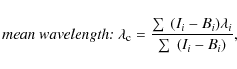
where Ii, Bi, and
The 1st-order moment represents the mean spectral position of
the profile. Since we are mainly interested in the relative
position, we subtracted the average (over the entire studied region)
mean position from the mean position of each profile. The resulting
value will be referred to as the 1st-order moment in our later
discussion. It corresponds to the Doppler shift in the case of a
Gaussian-shaped profile. However, in the case of Ly-![]() and Ly-
and Ly-![]() ,
not
only the Doppler shift of the line, but also the asymmetry of the
line profile can contribute to the 1st-order moment.
,
not
only the Doppler shift of the line, but also the asymmetry of the
line profile can contribute to the 1st-order moment.
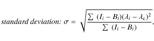
The 2nd-order moment is the standard deviation of the profile.
In the case of Ly-![]() and Ly-
and Ly-![]() ,
it includes information on both the
line width and the self-reversal depth. However, a narrow profile
with a deep self-reversal and a broad profile with a shallow
self-reversal may have a comparable value of the 2nd-order
moment. Since we wanted to avoid putting these two different kinds
of profiles into the same category, we did not analyse this moment
in our study.
,
it includes information on both the
line width and the self-reversal depth. However, a narrow profile
with a deep self-reversal and a broad profile with a shallow
self-reversal may have a comparable value of the 2nd-order
moment. Since we wanted to avoid putting these two different kinds
of profiles into the same category, we did not analyse this moment
in our study.
![\begin{figure}
\par\includegraphics[width=12.55cm,clip]{11445fg6.eps}
\end{figure}](/articles/aa/full_html/2009/34/aa11445-08/img29.png) |
Figure 6:
Various averaged Ly- |
| Open with DEXTER | |
![\begin{figure}
\par\includegraphics[width=16cm,clip]{11445fg7.eps}
\end{figure}](/articles/aa/full_html/2009/34/aa11445-08/img30.png) |
Figure 7: Dependence of the 1st and 3rd-order moments on the Doppler shifts of the Si III line (panels A to D) and O VI line (panels E to H). A positive and negative value of the Doppler shift indicates redshift (downflow) and blueshift (upflow), respectively. The error bar indicates the standard deviation of the corresponding moment in each bin. |
| Open with DEXTER | |
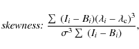
The 3rd-order moment, the skewness, is a measure of the
asymmetry of the line profiles. This parameter seems to be a good
candidate to study the asymmetry of Ly-![]() and Ly-
and Ly-![]() profiles. However,
both Ly-
profiles. However,
both Ly-![]() and Ly-
and Ly-![]() are blended with a He II line in the blue
wing. This blend will definitely influence the calculation of the
3rd-order moments. The problem for Ly-
are blended with a He II line in the blue
wing. This blend will definitely influence the calculation of the
3rd-order moments. The problem for Ly-![]() is even worse, since
the line is much narrower and weaker than Ly-
is even worse, since
the line is much narrower and weaker than Ly-![]() so that the
He II blend contributes more to the skewness of Ly-
so that the
He II blend contributes more to the skewness of Ly-![]() .
And
even more, there is another O I blend in the central part of
the Ly-
.
And
even more, there is another O I blend in the central part of
the Ly-![]() profile. The mixture effect of the blends can be seen in
the values calculated from Eq. (3). Therefore, these
values were adjusted by adding 0.05 for Ly-
profile. The mixture effect of the blends can be seen in
the values calculated from Eq. (3). Therefore, these
values were adjusted by adding 0.05 for Ly-![]() and subtracting 0.24
for Ly-
and subtracting 0.24
for Ly-![]() ,
to make those profiles with equal-height horns correspond
to a zero value of skewness.
,
to make those profiles with equal-height horns correspond
to a zero value of skewness.
We have sorted the profiles by each moment and defined six bins which were equally spaced in the moment. The average profiles in each bin are shown in Fig. 6. Again, only the results of the 1st and 3rd order moments, which we are mainly interested in, are presented. The averaged profiles exhibit obvious signatures of asymmetry, which will be further investigated in the next two sections.
5.2 Discussion
It is not easy to find a parameter which can purely reflect the
asymmetry of the Lyman line profiles. However, from Fig. 6
the 1st- and 3rd-order moments seem to reveal some
information, although not purely, on the line asymmetry. As
mentioned previously, both the shift of the entire profile and the
asymmetry of the profile can contribute to the 1st-order moment
of Ly-![]() and Ly-
and Ly-![]() .
A red-shifted profile with a stronger red wing
will definitely lead to a larger value of the 1st-order moment.
In contrast, a blue-shifted profile with a stronger blue wing should
correspond to a smaller value of the 1st-order moment. From
panels A and C of Fig. 5 we find that in statistical
sense, both Ly-
.
A red-shifted profile with a stronger red wing
will definitely lead to a larger value of the 1st-order moment.
In contrast, a blue-shifted profile with a stronger blue wing should
correspond to a smaller value of the 1st-order moment. From
panels A and C of Fig. 5 we find that in statistical
sense, both Ly-![]() and Ly-
and Ly-![]() have a larger value of their
1st-order moment in the network than in the internetwork. This
behaviour indicates that the average network-related profile is
either largely red-shifted or strongly enhanced in the red wing. As
mentioned previously, the 3rd-order moment, i.e., the skewness
of the Ly-
have a larger value of their
1st-order moment in the network than in the internetwork. This
behaviour indicates that the average network-related profile is
either largely red-shifted or strongly enhanced in the red wing. As
mentioned previously, the 3rd-order moment, i.e., the skewness
of the Ly-![]() and Ly-
and Ly-![]() profile, is influenced by the blends. However,
by inspection of Fig. 6 we find that the asymmetries of
the Lyman line profiles still can somehow be reflected in the values
of the 3rd-order moment. A negative/positive value of this
parameter corresponds to a profile with an enhanced red/blue horn.
profile, is influenced by the blends. However,
by inspection of Fig. 6 we find that the asymmetries of
the Lyman line profiles still can somehow be reflected in the values
of the 3rd-order moment. A negative/positive value of this
parameter corresponds to a profile with an enhanced red/blue horn.
![\begin{figure}
\par\includegraphics[width=12.5cm,clip]{11445fg8.eps}
\end{figure}](/articles/aa/full_html/2009/34/aa11445-08/img31.png) |
Figure 8:
Locations of the Ly- |
| Open with DEXTER | |
Since the asymmetries of the Lyman line profiles are caused by a
combined effect of Doppler shift and opacity (Gunár et al. 2008), we may
find that there is a relationship between the 1st and 3rd
order moments and the Doppler shift. Here we can only calculate the
Doppler shifts of two transition region lines, Si III and
O VI. In Fig. 7, we present the dependence of the
1st and 3rd order moments of Ly-![]() and Ly-
and Ly-![]() on the Doppler
shifts of Si III and O VI.
on the Doppler
shifts of Si III and O VI.
It is clear that the 1st-order moment of Ly-![]() is positively
correlated with the Doppler shift in the TR. This relationship is
corroborated by Fig. 8, in which locations of Ly-
is positively
correlated with the Doppler shift in the TR. This relationship is
corroborated by Fig. 8, in which locations of Ly-![]() profiles corresponding to the 25% smallest values (upper panels)
and 25% largest values (lower panels) of the 1st-order moment
are marked by red triangles on the Dopplergrams of Si III/
O VI. The white contours outline the network pattern as seen
on the Ly-
profiles corresponding to the 25% smallest values (upper panels)
and 25% largest values (lower panels) of the 1st-order moment
are marked by red triangles on the Dopplergrams of Si III/
O VI. The white contours outline the network pattern as seen
on the Ly-![]() radiance map. This strong correlation can be understood
if we assume that the Ly-
radiance map. This strong correlation can be understood
if we assume that the Ly-![]() profile is more redshifted and more
enhanced in the red horn in regions where larger TR downflows are
present. Panels D and H of Fig. 7 reveal a clear
decreasing trend of the skewness with increasing TR Doppler shift,
which means that the red horn of Ly-
profile is more redshifted and more
enhanced in the red horn in regions where larger TR downflows are
present. Panels D and H of Fig. 7 reveal a clear
decreasing trend of the skewness with increasing TR Doppler shift,
which means that the red horn of Ly-![]() tends to be more enhanced
where the Doppler shift is larger.
tends to be more enhanced
where the Doppler shift is larger.
To further substantiate this result, we extended the analysis on the
data set used for the spectral atlas of Curdt et al. (2001) and
completed a detailed wavelength calibration for Ly-![]() ,
based on
nearby fluorecence lines of neutral oxygen as wavelength standards.
These lines are radiatively excited, probably by Lyman continuum
photons via the 3s, 3d, and 4s levels of the O I triplet
system. We assume that these optically thin O I lines emerge
from the lower chromosphere (Avrett & Loeser 2008) and are at rest, at
least within the required uncertainties. We could reproduce the
average line profile with a multigauss fit of a broad Gaussian line
(
,
based on
nearby fluorecence lines of neutral oxygen as wavelength standards.
These lines are radiatively excited, probably by Lyman continuum
photons via the 3s, 3d, and 4s levels of the O I triplet
system. We assume that these optically thin O I lines emerge
from the lower chromosphere (Avrett & Loeser 2008) and are at rest, at
least within the required uncertainties. We could reproduce the
average line profile with a multigauss fit of a broad Gaussian line
(![]() 0.3 A FWHM) with a redshift of 5 km s-1, the He II
Balmer line in the blue wing, a much narrower Gaussian absorption
profile (
0.3 A FWHM) with a redshift of 5 km s-1, the He II
Balmer line in the blue wing, a much narrower Gaussian absorption
profile (![]() 0.15 A FWHM), and the O I lines as
wavelength standards. Because of the lack of wavelength standards
and the much stronger absorption, this method cannot be used for Ly-
0.15 A FWHM), and the O I lines as
wavelength standards. Because of the lack of wavelength standards
and the much stronger absorption, this method cannot be used for Ly-![]() .
.
This redshift of 5 km/s is comparable to the average redshift of a
typical TR line (Chae et al. 1998; Brekke et al. 1997; Warren et al. 1997; Xia 2003). In addition,
following the method described in Curdt et al. (2008a), we divided the
average network profile by the average internetwork profile and
obtained the network contrast profile for Ly-![]() (not shown here). We
found that there is a clear peak of this network contrast profile on
the red side of the line profile, which indicates that the Ly-
(not shown here). We
found that there is a clear peak of this network contrast profile on
the red side of the line profile, which indicates that the Ly-![]() line
is redshifted. Such a behaviour is similar to typical TR lines and a
natural result of the well-known brightness-Doppler-shift
relationship. Although the hydrogen Lyman lines are mainly formed in
the chromosphere and lower TR, since hydrogen is the most abundant
element in the solar atmosphere, there should still be some emission
sources of its resonance lines in the middle and upper TR. Ly-
line
is redshifted. Such a behaviour is similar to typical TR lines and a
natural result of the well-known brightness-Doppler-shift
relationship. Although the hydrogen Lyman lines are mainly formed in
the chromosphere and lower TR, since hydrogen is the most abundant
element in the solar atmosphere, there should still be some emission
sources of its resonance lines in the middle and upper TR. Ly-![]() is
optically thinner than Ly-
is
optically thinner than Ly-![]() ,
and we can see substantial Ly-
,
and we can see substantial Ly-![]() emission from the TR. That is why the behaviour of Ly-
emission from the TR. That is why the behaviour of Ly-![]() is similar
to typical TR lines.
is similar
to typical TR lines.
Panels B and F of Fig. 7 reveal a clear increasing trend
of the skewness with increasing TR Doppler shift, which means that
the blue horn of Ly-![]() tends to be more enhanced if the TR redshift
is larger. This is consistent with the result of Curdt et al. (2008b).
From panels A and E of Fig. 7 we find that the
1st-order moment of Ly-
tends to be more enhanced if the TR redshift
is larger. This is consistent with the result of Curdt et al. (2008b).
From panels A and E of Fig. 7 we find that the
1st-order moment of Ly-![]() tends to slightly increase or stay the
same with increasing TR Doppler shift. As we mentioned previously,
both the Doppler shift of the whole profile and the profile
asymmetry can contribute to the 1st-order moment. Since the
enhanced blue horn will reduce the moment, the only possibility is
that Ly-
tends to slightly increase or stay the
same with increasing TR Doppler shift. As we mentioned previously,
both the Doppler shift of the whole profile and the profile
asymmetry can contribute to the 1st-order moment. Since the
enhanced blue horn will reduce the moment, the only possibility is
that Ly-![]() is more redshifted in regions where larger downflows are
present.
is more redshifted in regions where larger downflows are
present.
The large scatters in Fig. 7 suggest that besides the TR
flows, there should be other effects which can influence the
asymmetry of the Lyman line profiles. We have to mention that the
explanation of the asymmetries of the Ly-![]() and Ly-
and Ly-![]() profiles will
require intricate modelling rather than simple imagination. Their
different asymmetries arise from the motions of the solar atmosphere
in its different layers as well as from the different line
opacities. Further theoretical work, especially modelling, is needed
to improve our understanding of the formation of the Lyman line
profiles.
profiles will
require intricate modelling rather than simple imagination. Their
different asymmetries arise from the motions of the solar atmosphere
in its different layers as well as from the different line
opacities. Further theoretical work, especially modelling, is needed
to improve our understanding of the formation of the Lyman line
profiles.
As mentioned above, energy losses through the Ly-![]() emission are the
most important radiative losses in the lower TR (Fontenla et al. 1988).
Thus the Ly-
emission are the
most important radiative losses in the lower TR (Fontenla et al. 1988).
Thus the Ly-![]() line should be important for the diagnostic of the
magnetic and plasma properties in the lower TR. It is still under
debate if the TR emission originates from a thin thermal interface
connecting the chromosphere and corona
(Dowdy et al. 1986; Peter 2001; Gabriel 1976), or from isolated unresolved
tiny loops (Feldman 1987,1983; Feldman & Laming 1994). Recently,
Patsourakos et al. (2007) reported the first spatially resolved
observations of subarcsecond-scale (0.3
line should be important for the diagnostic of the
magnetic and plasma properties in the lower TR. It is still under
debate if the TR emission originates from a thin thermal interface
connecting the chromosphere and corona
(Dowdy et al. 1986; Peter 2001; Gabriel 1976), or from isolated unresolved
tiny loops (Feldman 1987,1983; Feldman & Laming 1994). Recently,
Patsourakos et al. (2007) reported the first spatially resolved
observations of subarcsecond-scale (0.3
![]() )
loop-like
structures seen in the Ly-
)
loop-like
structures seen in the Ly-![]() line, as observed by the Very High
Angular Resolution Ultraviolet Telescope (VAULT). As mentioned in
that paper, flows can have distinct spectroscopic signatures, which
can help to distinguish between the two possibilities of the TR
emission origin. However, the signature of flows in the corona is
missing in the SUMER observation. Moreover, the spatial resolution
of our SUMER observation is still not high enough. Thus we can still
not make a final conclusion on the origin of the TR emission. We
think that only through a combined analysis of high-resolution
(subarcsecond) magnetic field, EUV imaging, and spectroscopic
observations can further substantial progress be expected.
line, as observed by the Very High
Angular Resolution Ultraviolet Telescope (VAULT). As mentioned in
that paper, flows can have distinct spectroscopic signatures, which
can help to distinguish between the two possibilities of the TR
emission origin. However, the signature of flows in the corona is
missing in the SUMER observation. Moreover, the spatial resolution
of our SUMER observation is still not high enough. Thus we can still
not make a final conclusion on the origin of the TR emission. We
think that only through a combined analysis of high-resolution
(subarcsecond) magnetic field, EUV imaging, and spectroscopic
observations can further substantial progress be expected.
6 Summary and conclusion
We have presented new results from a quasi-simultaneous observation
of the profiles of Ly-![]() and Ly-
and Ly-![]() .
We find that the self-absorption
in or around network is reduced, and in the internetwork region the
emissions tend to be more strongly absorbed in the central part of
the profiles. We suggest that the different magnetic structures in
the two regions might be responsible for this result. The outskirts
of the chromospheric and transition-region magnetic structures,
where the Lyman line emissions originate, are higher in the network
as compared to the internetwork.
.
We find that the self-absorption
in or around network is reduced, and in the internetwork region the
emissions tend to be more strongly absorbed in the central part of
the profiles. We suggest that the different magnetic structures in
the two regions might be responsible for this result. The outskirts
of the chromospheric and transition-region magnetic structures,
where the Lyman line emissions originate, are higher in the network
as compared to the internetwork.
Using the simultaneously measured photospheric magnetic field, we
could determine the ratio of Ly-![]() and Ly-
and Ly-![]() intensities for
different bins of magnetic field strength. Our result seems to
suggest that the ratio is independent of the magnetic field
strength.
intensities for
different bins of magnetic field strength. Our result seems to
suggest that the ratio is independent of the magnetic field
strength.
A rough inspection of the line profiles suggests that most
Ly-![]() profiles are stronger in their blue horn, while most Ly-
profiles are stronger in their blue horn, while most Ly-![]() profiles are stronger in their red horn. But the opposite
asymmetries of Ly-
profiles are stronger in their red horn. But the opposite
asymmetries of Ly-![]() and Ly-
and Ly-![]() are not strictly (on a pixel-to-pixel
level) correlated.
are not strictly (on a pixel-to-pixel
level) correlated.
The skewness of the profiles reveals clearly that the Ly-![]() and
Ly-
and
Ly-![]() profiles are more enhanced in the blue and red horns,
respectively, if larger TR downflows are present. The first-order
moment of Ly-
profiles are more enhanced in the blue and red horns,
respectively, if larger TR downflows are present. The first-order
moment of Ly-![]() is strongly correlated with the Doppler shift of
Si III and O VI. This result can be understood if
the profiles are more redshifted in regions where larger TR
downflows are present. The correlation is much weaker for Ly-
is strongly correlated with the Doppler shift of
Si III and O VI. This result can be understood if
the profiles are more redshifted in regions where larger TR
downflows are present. The correlation is much weaker for Ly-![]() ,
which indicates that the Ly-
,
which indicates that the Ly-![]() profiles should also be more
redshifted if larger TR downflows are present. Through a multi-Gauss
decomposition of Ly-
profiles should also be more
redshifted if larger TR downflows are present. Through a multi-Gauss
decomposition of Ly-![]() ,
we found that Ly-
,
we found that Ly-![]() is redshifted on average.
is redshifted on average.
The opposite asymmetries of the average profiles of Ly-![]() and Ly-
and Ly-![]() are presumably caused by the combined effects of flows in various
layers of the solar atmosphere and opacity difference of the two
lines. A mechanism for line formation can not be simply imagined but
must be thoroughly devised and further investigated by help of
models.
are presumably caused by the combined effects of flows in various
layers of the solar atmosphere and opacity difference of the two
lines. A mechanism for line formation can not be simply imagined but
must be thoroughly devised and further investigated by help of
models.
Acknowledgements
The SUMER project is financially supported by DLR, CNES, NASA, and the ESA PRODEX Programme (Swiss contribution). SUMER and MDI are instruments onboard SOHO, a mission operated by ESA and NASA. We thank the teams of SUMER and MDI for the spectroscopic and magnetic field data. We thank Dr. L.-D. Xia for the helpful discussion. We also thank the referee for his/her careful reading of the paper and for the comments and suggestions.H.T. is supported by the IMPRS graduate school run jointly by the Max Planck Society and the Universities of Göttingen and Braunschweig. The work of Hui Tian's group at PKU is supported by the National Natural Science Foundation of China (NSFC) under contract 40874090.
References
- Avrett, E. H., & Loeser, R. 2008, ApJS, 175, 229 [NASA ADS] [CrossRef] (In the text)
- Basri, G. S., Linsky, J. L., Bartoe, J.-D. F., Brueckner, G., & Van Hoosier. M. E. 1979, ApJ, 230, 924 [NASA ADS] [CrossRef] (In the text)
- Brekke, P., Hassler, D. M., & Wilhelm, K. 1997, Sol. Phys., 175, 349 [NASA ADS] [CrossRef]
- Chae, J., Schühle, U., & Lemaire, P. 1998, ApJ, 505, 957 [NASA ADS] [CrossRef]
- Curdt, W., Brekke, P., Feldman, U., et al. 2001, A&A, 375, 591 [NASA ADS] [CrossRef] [EDP Sciences] (In the text)
- Curdt, W., Tian, H., Dwivedi, B. N., & Marsch, E. 2008a, A&A, 491, L13 [NASA ADS] [CrossRef] [EDP Sciences] (In the text)
- Curdt, W., Tian, H., Teriaca, L., Schühle, U., & Lemaire, P. 2008b, A&A, 492, L9 [NASA ADS] [CrossRef] [EDP Sciences] (In the text)
- Dowdy, J. F., Jr., Rabin, D., & Moore, R. L. 1986, Sol. Phys., 105, 35 [NASA ADS] [CrossRef]
- Feldman, U. 1983, ApJ, 275, 367 [NASA ADS] [CrossRef]
- Feldman, U. 1987, ApJ, 320, 426 [NASA ADS] [CrossRef]
- Feldman, U., & Laming, J. M. 1994, ApJ, 434, 370 [NASA ADS] [CrossRef]
- Gabriel, A. H. 1976, Philos. Trans. R. Soc. London A, 28l, 575
- Emerich, C., Lemaire, P., Vial, J.-C., et al. 2005, Icarus 178, 429 (In the text)
- Fang, C., Feautrier, N., & Hénoux, J.-C. 1995, A&A, 297, 854 [NASA ADS]
- Fontenla, J. M., Reichmann, E. J., & Tandberg-Hanssen, E. 1988, ApJ 329, 464 (In the text)
- Fontenla, J. M., Avrett, E. H., & Loeser, E. 2002, ApJ, 572, 636 [NASA ADS] [CrossRef] (In the text)
- Gouttebroze, P., Lemaire, P., Vial, J.-C., & Artzner, G. 1978, ApJ, 225, 655 [NASA ADS] [CrossRef] (In the text)
- Gunár, S., Heinzel, P., Anzer,U., & Schmieder, B. 2008, A&A, 490, 307 [NASA ADS] [CrossRef] [EDP Sciences] (In the text)
- Gustafsson, M., Field, D., Lemaire, J. L., & Pijpers, F. P. 2006, A&A, 445, 601 [NASA ADS] [CrossRef] [EDP Sciences] (In the text)
- Heinzel, P., Schmieder, B.,Vial, J.-C., & Kotrc, P. 2001, A&A, 370, 281 [NASA ADS] [CrossRef] [EDP Sciences] (In the text)
- Heinzel, P., Anzer, U., & Gunár, S. 2005, A&A, 442, 331 [NASA ADS] [CrossRef] [EDP Sciences] (In the text)
- Hénoux, J.-C., Fang, C., & Gan, W.-Q. 1995, A&A, 297, 574 [NASA ADS]
- Lemaire, P., Charra, J., Jouchoux, A., et al. 1978, ApJ 223, L55
- Lemaire P., Wilhelm K., Curdt W., et al. 1997, Sol. Phys., 170, 105 [NASA ADS] [CrossRef]
- Lemaire, P., Emerich, C., Curdt, W., Schühle, U., & Wilhelm, K. 1998, A&A, 334, 1095 [NASA ADS] (In the text)
- Lemaire, P., Emerich, C., Vial, J.-C., et al. 2002, in Proc. SOHO 11 From Solar Min to Max: Half a Solar Cycle with SOHO, ed. A. Wilson, Davos, Switzerland, ESA SP-508, 219 (In the text)
- Lemaire, P., Emerich, C., Vial, J.-C., et al. 2005, AdSpR, 35, L384 [NASA ADS]
- Mariska, J. T. 1992, The Solar Transition Region (Cambridge: Cambridge Univ. Press)
- Marsch, E., Tu, C.-Y., Heinzel, P., Wilhelm, K., & Curdt, W. 1999, A&A, 347, 676 [NASA ADS] (In the text)
- Marsch, E., Tu,C.-Y., & Wilhelm, K. 2000, A&A, 359, 381 [NASA ADS] (In the text)
- Nicolas, K. R., Kjeldseth Moe, O., & Tousey, R. 1976, JGR, 81, 3465 [NASA ADS] [CrossRef] (In the text)
- Patsourakos, S., Gouttebroze, P., & Vourlidas, A. 2007, ApJ, 664, 1214 [NASA ADS] [CrossRef] (In the text)
- Peter, H. 2001, A&A, 374, 1108 [NASA ADS] [CrossRef] [EDP Sciences] (In the text)
- Scherrer, P. H., Bogart, R. S., Bush, R. I., et al. 1995, Sol. Phys., 162,129 (In the text)
- Schmieder, B., Heinzel, P., Vial, J.-C., & Rudway, P. 1999, Sol. Phys., 189, 109 [NASA ADS] [CrossRef] (In the text)
- Schmieder, B., Gunár, S., Heinzel, P., & Anzer, U. 2007, Sol. Phys., 241, 53 [NASA ADS] [CrossRef] (In the text)
- Teriaca, L., Schühle, U., Solanki, S. K., Curdt, W., & Marsch, E. 2005a, in Proc. Chromospheric and Coronal Magnetic Fields, ed. D. E., Innes, A., Lagg, & S. K., Solanki (Germany: Katlenburg-Lindau), ESA SP-596, 66
- Teriaca, L., Schühle, U., Solanki, S. K., Curdt, W., & Marsch, E. 2005b, in Proc. ESPM The Dynamic Sun: Challenges for Theory and Observations, ed. D., Danesy, S., Poedts, A., De Groof, & J., Andries, Leuven, Belgium, ESA SP-60, 100
- Teriaca, L., Schühle, U., Solanki, S. K., Curdt, W.,& Marsch, E. 2006, in Proc. 10 years of SoHO and beyond, ed. H., Lacoste, & L., Ouwehand, Giardini-Naxos, Italy, ESA SP-617, 77
- Tian, H., Curdt, W., Teriaca, L., Landi, E., & Marsch, E. 2009, A&A, [DOI:10.1051/0004-6361/200912114]
- Vernazza, J. E., & Reeves, E. M. 1978, ApJS, 37, 485 [NASA ADS] [CrossRef] (In the text)
- Vidal-Madjar, A. 1975, Sol. Phys. 40, 69 (In the text)
- Vial, J.-C. 1982, ApJ, 253, 330 [NASA ADS] [CrossRef]
- Vial, J.-C., Ebadi, H., & Ajabshirizadeh, A. 2007, Sol. Phys., 246, 327 [NASA ADS] [CrossRef] (In the text)
- Warren, H. P., Mariska, J. T., Wilhelm, K., & Lemaire, P. 1997, ApJ, 484, L91 [NASA ADS] [CrossRef]
- Warren, H. P., Mariska, J. T., & Wilhelm, K. 1998, ApJS, 119, 105 [NASA ADS] [CrossRef] (In the text)
- Wilhelm, K., Curdt, W., Marsch, E., et al., 1995, Sol. Phys., 162, 189 [NASA ADS] [CrossRef]
- Wilhelm, K., Lemaire, P., Dammasch, I. E., et al., 1998, A&A, 334,685 (In the text)
- Xia, L.-D. 2003, Ph.D. Thesis (Göttingen: Georg-August-Univ.) (In the text)
- Xia, L.-D., Marsch, E., & Wilhelm, K. 2004, A&A, 424, 1025 [NASA ADS] [CrossRef] [EDP Sciences] (In the text)
All Tables
Table 1:
The observed ratios between Ly-![]() and Ly-
and Ly-![]() photon
radiances.
photon
radiances.
All Figures
| |
Figure 1:
Radiance maps of two Lyman and two transition-region lines:
(A) Ly- |
| Open with DEXTER | |
| In the text | |
| |
Figure 2:
Maps of the self-reversal depth (represented by
|
| Open with DEXTER | |
| In the text | |
| |
Figure 3:
Positions of Ly- |
| Open with DEXTER | |
| In the text | |
| |
Figure 4:
Upper panels A to C: scatter plot of the relationship
between the Ly- |
| Open with DEXTER | |
| In the text | |
| |
Figure 5:
Maps of the 1st (A, C) and 3rd (B, D) order
moments, as described in the text, of the Ly- |
| Open with DEXTER | |
| In the text | |
| |
Figure 6:
Various averaged Ly- |
| Open with DEXTER | |
| In the text | |
| |
Figure 7: Dependence of the 1st and 3rd-order moments on the Doppler shifts of the Si III line (panels A to D) and O VI line (panels E to H). A positive and negative value of the Doppler shift indicates redshift (downflow) and blueshift (upflow), respectively. The error bar indicates the standard deviation of the corresponding moment in each bin. |
| Open with DEXTER | |
| In the text | |
| |
Figure 8:
Locations of the Ly- |
| Open with DEXTER | |
| In the text | |
Copyright ESO 2009
Current usage metrics show cumulative count of Article Views (full-text article views including HTML views, PDF and ePub downloads, according to the available data) and Abstracts Views on Vision4Press platform.
Data correspond to usage on the plateform after 2015. The current usage metrics is available 48-96 hours after online publication and is updated daily on week days.
Initial download of the metrics may take a while.