| Issue |
A&A
Volume 504, Number 1, September II 2009
|
|
|---|---|---|
| Page(s) | 161 - 170 | |
| Section | Stellar structure and evolution | |
| DOI | https://doi.org/10.1051/0004-6361/200811144 | |
| Published online | 09 July 2009 | |
Structure and evolution of rotationally and tidally distorted stars
H. F. Song1,2 - Z. Zhong1 - Y. Lu1
1 - College of science, Guizhou University, Guiyang, 550025, PR China
2 -
Joint Centre for Astronomy, National Astronomical Observatories-Guizhou University, Guiyang, 550025, PR China
Received 14 October 2008 / Accepted 2 June 2009
Abstract
Aims. This paper aims to study the configuration of two components caused by rotational and tidal distortions in the model of a binary system.
Methods. The potentials of the two distorted components can be approximated to 2nd-degree harmonics. Furthermore, both the accretion luminosity (
![]() )
and the irradiative luminosity are included in stellar structure equations.
)
and the irradiative luminosity are included in stellar structure equations.
Results. The equilibrium structure of rotationally and tidally distorted star is exactly a triaxial ellipsoids. A formula describing the isobars is presented, and the rotational velocity and the gravitational acceleration at the primary surface simulated. The results show the distortion at the outer layers of the primary increases with temporal variation and system evolution. Besides, it was observed that the luminosity accretion is unstable, and the curve of the energy-generation rate fluctuates after the main sequence in rotation sequences. The luminosity in rotation sequences is slightly weaker than that in non-rotation sequences. As a result, the volume expands slowly. Polar ejection is intensified by the tidal effect. The ejection of an equatorial ring may be favoured by both the opacity effect and the
![]() -effect in the binary system.
-effect in the binary system.
Key words: stars: rotation - stars: binaries: close
1 Introduction
In the conventional model of binary stars, there is no consideration
of spin and tidal effects (Eggleton 1971, 1972, 1973; Hofmeister
et al. 1964; Kippenhahn et al. 1967; etc.); however,
rotation and tide have been regarded as two important physical
factors in recent years, so they need to be considered for a better
understanding of the evolution of massive close binaries (e.g.,
Heger et al. 2000a; Meynet & Maeder 2000). The
structure and evolution of rotating single stars has been studied by
many investigators (Kippenhahn & Thomas 1970; Endal
& Sofia 1976; Pinsonneaul et al. 1989;
Meynet & Maeder 1997; Langer 1998, 1999; Huang 2004a).
However, it is also very important to study the evolution of
rotating binary stars (Jackson 1970; Chan & Chau 1979; Langer 2003; Huang 2004b; Petrovic et al. 2005a,b; Yoon et al. 2006). The effect of spin on structure equations has been investigated (e.g. the
present Eggleton's stellar evolution code; Li et al. 2004a,b, 2005; K
![]() hler 2002). They adopted the lowest-order approximate analysis in which two components were treated as spherical stars. In fact, with the joint effects of spin and tide, the structure of a star changes from spherically symmetric to non-spherically symmetric. Then, the stellar structure equations become three dimensional. Theory distinguishes two components in the tide, namely equilibrium tide (Zahn 1966) and the dynamical tide (Zahn 1975). Then, the dissipation mechanisms acting on those tides, namely the viscous friction for the equilibrium tide and the radiative damping for the dynamical tide, have been identified (Zahn 1966, 1975, 1977). The distortion throughout the outer regions of the two components is not small in short-period binary systems. The higher-order terms in the external gravitational field should not be ignored (Jackson 1970).
hler 2002). They adopted the lowest-order approximate analysis in which two components were treated as spherical stars. In fact, with the joint effects of spin and tide, the structure of a star changes from spherically symmetric to non-spherically symmetric. Then, the stellar structure equations become three dimensional. Theory distinguishes two components in the tide, namely equilibrium tide (Zahn 1966) and the dynamical tide (Zahn 1975). Then, the dissipation mechanisms acting on those tides, namely the viscous friction for the equilibrium tide and the radiative damping for the dynamical tide, have been identified (Zahn 1966, 1975, 1977). The distortion throughout the outer regions of the two components is not small in short-period binary systems. The higher-order terms in the external gravitational field should not be ignored (Jackson 1970).
It is a very complex process to determine the equilibrium structure
of the two components. Therefore, approximate methods have been
widely adopted for studying these effects. In 1933, the theory of
distorted polytropes was introduced by Chandrasekhar. Kopal
(1972, 1974) developed the concept of Roche equipotential and of
Roche coordinates to analyse the problem of rotationally and tidally
distorted stars in a binary system. Bur
![]() a (1989a, 1988)
took advantage of the high-order perturbing potential to describe
rotational and tidal deformations to discuss the figures and dynamic
parameters of synchronously orbiting satellites in the solar system.
The equilibrium structure of the two components were treated as two
non-symmetric rotational ellipsoids with two different semi-major
axes a1 and a2 (
a1>a2) by Huang (2004b). It is
very important that Kippenhahn & Thomas (1970) introduced a
method of simplifying the two-dimensional model with conservative
rotation and allowed the structure equations for a one-dimensional
star to incorporate the hydrostatic effect of rotation. This method
has been adopted by Endal & Sofia (1976) and Meynet & Maeder
(1997), who applied it to the case of shellular rotation law (Zahn
1992). In this case, the rotation rate takes the simplified form of
a (1989a, 1988)
took advantage of the high-order perturbing potential to describe
rotational and tidal deformations to discuss the figures and dynamic
parameters of synchronously orbiting satellites in the solar system.
The equilibrium structure of the two components were treated as two
non-symmetric rotational ellipsoids with two different semi-major
axes a1 and a2 (
a1>a2) by Huang (2004b). It is
very important that Kippenhahn & Thomas (1970) introduced a
method of simplifying the two-dimensional model with conservative
rotation and allowed the structure equations for a one-dimensional
star to incorporate the hydrostatic effect of rotation. This method
has been adopted by Endal & Sofia (1976) and Meynet & Maeder
(1997), who applied it to the case of shellular rotation law (Zahn
1992). In this case, the rotation rate takes the simplified form of
![]() .
It was demonstrated that the shape of an isobar
in the case of the shellular rotation law is identical to one of the
equipotentials in the conservative case of Meynet & Maeder
(1997).
.
It was demonstrated that the shape of an isobar
in the case of the shellular rotation law is identical to one of the
equipotentials in the conservative case of Meynet & Maeder
(1997).
At the semi-detached stage, both mass transfer between the components and luminosity change of a secondary exist due to the release of accretion energy which is correlative with the external potential of the two components. When the joint effect of rotation and tide are considered, the potential of the two components are different from those in non-rotational cases. Therefore, the luminosity due to the release of accretion energy, as well as irradiation energy, can significantly alter the structure and evolution of the secondary. In a rotating star, meridional circulation and shear turbulence exist, both of which can drive the transport of chemical elements. This effect is stronger and has already been studied by many scholars (Endal & Sofia 1978; Pinsonneaul et al. 1989; Chaboyer & Zahn 1992; Zahn 1992; Meynet & Maeder 1997; Maeder 2000; Meader & Zahn 1998; Maeder & Meynet 2000; Denissenkov et al. 1999; Talon et al. 1997; Decressin et al. 2009). In this paper, the amplitude expression for the radial component of the meridional circulation velocity U(r) considers the effect of tidal force, which may be important in a massive close binary system.
This paper is divided into four main sections. In Sect. 2, the structure equations of rotating binary stars are presented. Material diffusion equations and boundary conditions are provided. Then, the accretion luminosity, including gravitational energy, heat energy, and radiation energy, is deduced. In Sect. 3, the results of numerical calculation are described and discussed in detail. In Sect. 4, conclusions are drawn.
2 Model for rotating binary stars
2.1 Potential of rotating binary stars
It is well known that the rotation of a component is synchronous
with the orbital motion of a system thanks to a strong tidal effect.
Such synchronous rotation also exists inside the component (Giuricin
et al. 1984; Van Hamme & Wilson 1990); therefore,
conventional theories usually assume that two components rotate
synchronously and revolve in circular orbits (Kippenhahn & Weigert
1967; De Loore 1980; Huang & Taam
1990; Vanbeveren 1991; De Greve 1993). A coordinate system rotating with the orbital angular
velocity of the stars is introduced. The mass centre of the primary
is regarded as the origin, and it is presumed that the z-axis is
perpendicular to the orbital plane, and the positive x-axis
penetrates the mass centre of the secondary. The gravitational
potential at any point
![]() of the surface of the
primary can be approximately expressed as
of the surface of the
primary can be approximately expressed as
 |
(1) |
where V is the gravitational potential and given by Bur
![$\displaystyle V=\frac{GM_{1}}{r_{p}}\left[\frac{r_{p}}{r}\!+\!\left(\frac{r_{p}...
...frac{r_{p}}{r}\right)^{3}J_{2}^{(2)}P_{2}^{2}(\cos\theta)\cos
2\varphi\right ].$](/articles/aa/full_html/2009/34/aa11144-08/img17.png) |
(2) |
Here,
![\begin{displaymath}V_{\rm t}=\frac{GM_{2}}{D}\left(\frac{r}{D}\right)^{2}\left[-...
...s\theta)+\frac{1}{4}P_{2}^{2}(\cos\theta)\cos 2\varphi\right],
\end{displaymath}](/articles/aa/full_html/2009/34/aa11144-08/img19.png) |
(3) |
where it is assumed that the mean equatorial radius equals that of the equivalent sphere in the above equation for the convenience of calculation. Both M1 and M2 are the mass of the primary and the secondary, respectively, and rp represents each equivalent radius inside the star,
| (4) |
where J2(0) and J2(2) are dimensionless stokes parameters. If M1 can generally be negligible compared to M2, the stokes parameters can be expressed as (Bur
![\begin{displaymath}J_{2}^{(0)}=-\left[\frac{1}{3}k_{{\rm s}}+\frac{1}{2}k_{{\rm t}}\right]q\left(\frac{r_{p}}{D}\right)^{3}=-J_{2},
\end{displaymath}](/articles/aa/full_html/2009/34/aa11144-08/img26.png) |
(5) |
 |
(6) |
where
| |
= |  |
(7) |
![$\displaystyle + \frac{1}{4}q\left(\frac{r_{1}}{D}\right)^{2}\left [3\sin^{2}\theta(1+\cos2\varphi)-2 \right]\bigg\}.$](/articles/aa/full_html/2009/34/aa11144-08/img36.png) |
The potential of the secondary is deduced by substituting M2for M1 and
2.2 Considering stellar structure equations with spin and tidal effects
The spin of the two components is rigid rotation, and it belongs to
conservative rotation. The definition of equivalent sphere was
adopted in a practical calculation. Therefore, the triaxial
ellipsoid model is simplified to a one-dimensional model. The
structure equations are presented as
 |
(8) |
 |
(9) |
 |
(10) |
where
| (11) |
where
 |
(12) |
 |
(13) |
 |
(14) |
 |
(15) |
where
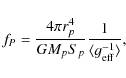
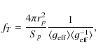
2.3 Calculation of quantities fP and fT
2.3.1 Shape and gravitational acceleration of triaxial ellipsoid
To obtain the factors fP and fT, the mean values
![]() and
and
![]() over the isobar surface have to be calculated.
Therefore, the shape of isobars must be given first. The functions
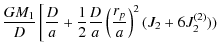
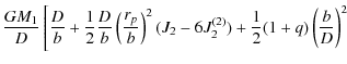
for the semi-major axes a, b, and c to the radius of the
equivalent sphere rP can be obtained from Eq. (7) as
over the isobar surface have to be calculated.
Therefore, the shape of isobars must be given first. The functions
for the semi-major axes a, b, and c to the radius of the
equivalent sphere rP can be obtained from Eq. (7) as
 |
(16) |
 |
|||
![$\displaystyle \quad+ \left. \frac{1}{2}(1+q)\left(\frac{a}{D}\right)^{2}+q\left(\frac{a}{D}\right)^{2}\right]
=\frac{GM_1}D\left[ \frac{D}{c} \right.\nonumber$](/articles/aa/full_html/2009/34/aa11144-08/img56.png) |
|||
![$\displaystyle \quad+\left.\frac 12
\frac{D}{c}\left(\frac{r_{p}}{c}\right)^{2}(-2J_{2})
- \frac{1}{2}q\left(\frac{c}{D}\right)^{2}\right],$](/articles/aa/full_html/2009/34/aa11144-08/img57.png) |
(17) |
 |
|||
![$\displaystyle \quad-\left.\frac{1}{2}q(\frac{b}{D})^{2}\right]=\frac{GM_1}D\lef...
...frac{D}{c}+\frac 12 \frac{D}{c}\left(\frac{r_{p}}{c}\right)^{2}(-2J_{2})\right.$](/articles/aa/full_html/2009/34/aa11144-08/img59.png) |
|||
![$\displaystyle \quad- \left.\frac{1}{2}q\left(\frac{c}{D}\right)^{2}\right].$](/articles/aa/full_html/2009/34/aa11144-08/img60.png) |
(18) |
The left hand side of Eq. (17) corresponds to
 |
|||
 |
(19) |
| |
= |  |
|
![$\displaystyle \times(2\cos^{2}\varphi-1)]-(1+q)\frac{r}{D}
-3q\frac{r}{D}\cos^{2}\varphi \bigg\}\sin\theta \cos\theta ,$](/articles/aa/full_html/2009/34/aa11144-08/img69.png) |
(20) |
| |
= |  |
|
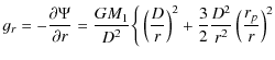
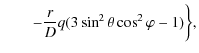
| = | ![$\displaystyle \frac{GM_{1}}{D^{2}}\left[12\left(\frac{D}{r}\right)^{2}\left(\fr...
...}\right)^{2}J_{2}^{(2)}+3q\frac{r}{D}\right]\sin\theta \cos\varphi \sin\varphi.$](/articles/aa/full_html/2009/34/aa11144-08/img72.png) |
(21) |
However, the total potential in the stellar interior (to first-order approximation) can be composed by four parts (Kopal 1959, 1960, 1974; Endal & Sofia 1976; Landin 2009):
| |
= | ||
| = | ![$\displaystyle \frac{GM_{\psi}}{r}+\frac{1}{2}\omega^{2}r^{2}\sin^{2}\theta
+\fr...
..._{j=2}^{4}\left(\frac{r_{0}}{D}\right)^{j}P_{j}(\sin\theta\cos
\varphi )\right]$](/articles/aa/full_html/2009/34/aa11144-08/img79.png) |
||
 |
|||
 |
(22) |
The quantity
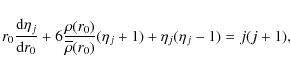 |
(23) |
for j=2,3,4, and boundary condition
![\begin{displaymath}g_{i}=\left[\left(\frac{\partial \psi}{\partial
r}\right)^{2}...
...partial
\varphi}\right)^{2}\right]^{\frac{1}{2}},~~~ (i=1, 2).
\end{displaymath}](/articles/aa/full_html/2009/34/aa11144-08/img85.png) |
(24) |
The integral in above equations and their derivatives must be evaluated numerically. The mean values of
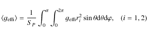 |
(25) |
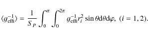 |
(26) |
According to Eqs. (13) and (14), the values of fP and fT can be obtained when the mean values
 |
(27) |
The surface area Sp of the isobar can be expressed as
 |
(28) |
2.4 Element diffusion process
The effect of meridian circulation can drive the transport of
chemical elements and angular momentum in rotating stars. For the
components in solid-body rotation, no differential rotation exists
that can cause shear turbulence. According to Endal & Sofia (1978)
and Pinsonneault (1989), the transport of chemical composition is
treated as a diffusion process. The equation takes the form of
(Chaboyer & Zahn 1992)
![$\displaystyle \left( \frac{\partial y_\alpha }{\partial t}\right) =\frac{1}{\rh...
...ght)\right] +\left(
\frac{\partial y_\alpha }{\partial t}\right) _{{\rm nuc }},$](/articles/aa/full_html/2009/34/aa11144-08/img92.png) |
(29) |
where
| (30) |
where
| U(r) | = |  |
(31) |
 |
where the term
There is no source or sink at the inner and the outer boundaries of
the two components. Therefore, the boundary conditions are used as
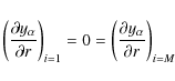 |
(32) |
where the subscript i denotes different layers inside stars. The initial abundance equals the one at the zero-age main sequence. Therefore, the initial condition is
| (33) |
Table 1: Parameters at different evolutionary points a, b, c, d, e, and f in sequences of cases 1 and 2.
2.5 Luminosity accretion
In the case where the joint effect of rotation and tide is ignored,
the two components are spherically symmetric. The star fills its
Roche lobe and begins to transfer matter to the companion. However,
in the case with the effects of rotation and tide being considered,
the components are triaxial ellipsoids. The condition for the mass
overflow through Roche lobe flow should be revised as
![]() (Huang 2004b). It is assumed that the transferred mass is
distributed within a thin shell at the surface of the primary before
the transfer, and within a thin shell at the surface of the
secondary after the transfer. Three forms of energy (including
potential energy, heat energy, and radiative energy) are transferred
to the secondary. The mass transfer rate is
(Huang 2004b). It is assumed that the transferred mass is
distributed within a thin shell at the surface of the primary before
the transfer, and within a thin shell at the surface of the
secondary after the transfer. Three forms of energy (including
potential energy, heat energy, and radiative energy) are transferred
to the secondary. The mass transfer rate is ![]() .
Two different
cases are considered:
.
Two different
cases are considered:
- a)
- If the joint effect of rotation and tide is ignored, the
accretion luminosity can be expressed directly in terms of the Roche
lobe potential at the inner Lagrangian point,
 ,
and at
the surface of the secondary
,
and at
the surface of the secondary
 (Han & Webbink 1999):

= 
![$\displaystyle \left.-\frac{1+q}{2}\left(1-\frac{R_{2}}{D}-\frac{q}{1+q}\right)^2
\bigg)\right],$](/articles/aa/full_html/2009/34/aa11144-08/img124.png)
(34)
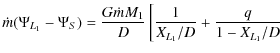
where XL1 is the distance between the primary and L1, and R2 is the radius of the secondary. - b)
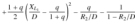
- If the joint effect of rotation and tide is considered, the
equilibrium structure of the two components will be treated as
triaxial ellipsoids. The release of potential energy because of the
accretion of a mass rate
 to the secondary is given by
= 
![$\displaystyle \left.\times\left(2J_{2}^{0}\right)-\frac{1}{2}q
\left(\frac{c_{2}}{D}\right)^{2}\right],$](/articles/aa/full_html/2009/34/aa11144-08/img126.png)
(35)
where
is the potential of the secondary. Similarly, as
the two components have different temperatures, the transmitted
thermal energy will be
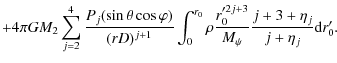
(36)
where and
and
 represent the effective temperature
of the primary and the secondary, respectively, and
represent the effective temperature
of the primary and the secondary, respectively, and  and
and
 are the mean molecular weights of the primary and the
secondary, respectively.
are the mean molecular weights of the primary and the
secondary, respectively.  refers to proton mass. Because of
the irradiation, energy accumulated by the primary and the secondary
can be given by (Huang & Taam 1990)
refers to proton mass. Because of
the irradiation, energy accumulated by the primary and the secondary
can be given by (Huang & Taam 1990)
![\begin{displaymath}\triangle L_{r,1,2}=
\frac{1}{2}\left[1-(D^{2}-R_{1,2}^{2})^{\frac{1}{2}}/D\right]L_{2,1},
\end{displaymath}](/articles/aa/full_html/2009/34/aa11144-08/img133.png)
(37)
where R1 and R2 are the radii of the primary and the secondary, and L1 and L2 are the luminosities of the primary and the secondary, respectively. The total accretion luminosity is
(38)
Because a part of the total energy may be dissipated dynamically, is assumed to range from 0.1 to 0.5 (Huang 1993). A
value
is assumed to range from 0.1 to 0.5 (Huang 1993). A
value  is adopted.
3 Results of numerical calculation
The structure and evolution of binary system was traced with the
modified version of a stellar structure program, which was developed
by Kippenhahn et al. (1967) and has been updated to include mass
and energy transfer processes. The calculation method is based on
the technique of Kippenhahn & Thomas (1970) and takes advantage of
the concept of isobar (Zahn 1992; Meynet & Maeder 1997). Both
components of the binary are calculated simultaneously. The initial
mass of the system components is set at 9 ![]() and
6
and
6 ![]() .
The initial chemical composition X equals X=0.70, and
Z=0.02 is adopted for the two components. Similarly, the initial
orbital separation between the two components for all sequences is
defined as 20.771
.
The initial chemical composition X equals X=0.70, and
Z=0.02 is adopted for the two components. Similarly, the initial
orbital separation between the two components for all sequences is
defined as 20.771 ![]() ,
so mass transfer via Roche lobe occurs
in case A (at the central hydrogen-burning phase of the primary).
Two evolutionary sequences corresponding to the evolution with the
joint effect of rotation and tide being considered or ignored are
calculated. The sequence denoted by case 1 represents the evolution
without the effects of rotation and tide being considered, while the
sequence denoted by case 2 represents the evolution with the effects
of rotation and tide being considered. The calculation of Roche lobe
is taken from the study by Huang & Taam (1990). The
non-conservative evolution in the two cases was considered. Because
the local flux at colatitude
,
so mass transfer via Roche lobe occurs
in case A (at the central hydrogen-burning phase of the primary).
Two evolutionary sequences corresponding to the evolution with the
joint effect of rotation and tide being considered or ignored are
calculated. The sequence denoted by case 1 represents the evolution
without the effects of rotation and tide being considered, while the
sequence denoted by case 2 represents the evolution with the effects
of rotation and tide being considered. The calculation of Roche lobe
is taken from the study by Huang & Taam (1990). The
non-conservative evolution in the two cases was considered. Because
the local flux at colatitude ![]() is proportional to the
effective gravity
is proportional to the
effective gravity ![]() according to Von Zeipel theorem (Maeder
1998), the mass-loss rate due to the stellar winds intensified by
tidal, rotational, and irradiative effects is obtained according to
Huang & Taam (1990; cf. Table 1). The angular velocity of the system
and the orbital separation between the two components change due to
a number of factors: changes in physical processes as the binary
system evolves, including the loss of mass and angular momentum via
stellar winds, mass transfer via Roche lobe overflow, exchange of
angular momentum between component rotation and the orbital motion
of the system caused by tidal effect, and changes in moments of
inertia of the components. The changes in the angular velocity of
the system and the orbital separation between the two components can
be calculated according to Huang & Taam (1990), and the results are
listed in Table 1. Other parameters are treated in the same way for
two sequences.
according to Von Zeipel theorem (Maeder
1998), the mass-loss rate due to the stellar winds intensified by
tidal, rotational, and irradiative effects is obtained according to
Huang & Taam (1990; cf. Table 1). The angular velocity of the system
and the orbital separation between the two components change due to
a number of factors: changes in physical processes as the binary
system evolves, including the loss of mass and angular momentum via
stellar winds, mass transfer via Roche lobe overflow, exchange of
angular momentum between component rotation and the orbital motion
of the system caused by tidal effect, and changes in moments of
inertia of the components. The changes in the angular velocity of
the system and the orbital separation between the two components can
be calculated according to Huang & Taam (1990), and the results are
listed in Table 1. Other parameters are treated in the same way for
two sequences.
![\begin{figure}
\par\mbox{\includegraphics[width=7.4cm,clip]{11144fig1.eps}\inclu...
...11144fig3.eps}\includegraphics[width=7.4cm,clip]{11144fig4.eps} }
\end{figure}](/articles/aa/full_html/2009/34/aa11144-08/img140.png) |
Figure 1:
Surface rotating velocity distribution of primary varying
with time. Four panels a), b), c), and d) correspond to periods:
2.776, 2.760, 2.746, and 2.628 days, and corresponding
evolutive time is 0,
|
| Open with DEXTER | |
The evolution of the binary system proceeded as follows (cf. Table 1). Evolutionary time, orbital period, mass of two stars,
luminosities and effective temperature of two stars, central and
surface helium mass fraction of the primary, and mean equatorial
rotational velocities of two stars are listed in Table 1. Points a,
b, c, d, e, and f denote the zero-age main sequence, the beginning
of the mass transfer stage, the beginning of H-shell burning, the
end of central hydrogen-burning, the beginning of the central
helium-burning stage, and the end of calculation, respectively. At
the beginning of mass exchange, the luminosity and effective
temperature of the primary component decrease rapidly. The secondary
accretes
![]() for case 1 and
for case 1 and
![]() for case 2
during the mass transfer in case A. Because of this mass gain, the
luminosity and the temperature of the secondary go up. When the mass
is transferred from the more massive star to the less massive one,
the separation between the centres of the two components as well as
the orbital period of the system decrease. Some orbital angular
momentum is transformed into the spin angular momentum of both
components, and this process is crucial to model the spin-up of the
accretion star. With mass overflow, the mass of the primary will be
less than that of the secondary. When the mass is transferred from
the less massive star to the more massive one, the separation
between the centres of the two components as well as the orbital
period of the system increases. Some spin angular momenta in both of
the components are transformed into orbital angular momentum. This
physical process results in a longer epilogue after mass transfer.
for case 2
during the mass transfer in case A. Because of this mass gain, the
luminosity and the temperature of the secondary go up. When the mass
is transferred from the more massive star to the less massive one,
the separation between the centres of the two components as well as
the orbital period of the system decrease. Some orbital angular
momentum is transformed into the spin angular momentum of both
components, and this process is crucial to model the spin-up of the
accretion star. With mass overflow, the mass of the primary will be
less than that of the secondary. When the mass is transferred from
the less massive star to the more massive one, the separation
between the centres of the two components as well as the orbital
period of the system increases. Some spin angular momenta in both of
the components are transformed into orbital angular momentum. This
physical process results in a longer epilogue after mass transfer.
![\begin{figure}
\par\mbox{\includegraphics[width=7.5cm,clip]{11144fig5.eps}\inclu...
...fig9.eps}\includegraphics[width=7.5cm,clip]{11144fig10.eps} }
\par
\end{figure}](/articles/aa/full_html/2009/34/aa11144-08/img144.png) |
Figure 2:
Variation of relative gravitational accelerations at the
surface of primary under coordinate |
| Open with DEXTER | |
The equilibrium configuration deviates from spherical symmetry
because of the centrifugal forces and tidal forces. And the deviated
region mainly lies in the outer layer of a star. In fact, the
distorted stellar surface forms the shape of a triaxial ellipsoid. A
distorted isobar surface can be expressed as
![\begin{displaymath}r=r_{p}[1+f(r)P_{2}(\cos\theta)+g(r)P_{2}^{2}(\cos\theta)\cos2\varphi],
\end{displaymath}](/articles/aa/full_html/2009/34/aa11144-08/img145.png) |
(39) |
which corresponds to the form of the disturbing potential (Zahn 1992). The coefficients f(r) and g(r) can be defined as
The variation relative gravitational accelerations, the tidal force,
and the ratio of
![]() on the surface of the primary
under the coordinate
on the surface of the primary
under the coordinate ![]() and
and ![]() at the beginning of mass
overflow are shown in Fig. 2. The quantities gr,
at the beginning of mass
overflow are shown in Fig. 2. The quantities gr,
![]() ,
and
,
and
![]() are the three components of gravitational
acceleration. The six panels (a), (b), (c), (d), (e), and (f)
represent the distribution of gr/g,
are the three components of gravitational
acceleration. The six panels (a), (b), (c), (d), (e), and (f)
represent the distribution of gr/g,
![]() ,
,
![]() ,
,
![]() ,
,
![]() ,
and
,
and
![]() ,
respectively. The quantity g equals the gravitational
acceleration of the corresponding equivalent sphere
(
,
respectively. The quantity g equals the gravitational
acceleration of the corresponding equivalent sphere
(
![]() ). When the joint effect of rotation
and tide is considered, the gravitational accelerations are
different from those in the conventional model. Gravitational
acceleration generally has three components.
). When the joint effect of rotation
and tide is considered, the gravitational accelerations are
different from those in the conventional model. Gravitational
acceleration generally has three components.
![\begin{figure}
\par\includegraphics[width=6.5cm,clip]{11144fig11.eps}\includegraphics[width=6.5cm,clip]{11144fig12.eps}
\end{figure}](/articles/aa/full_html/2009/34/aa11144-08/img163.png) |
Figure 3: Time variation of relative accretion luminosity at semi-detached stage. Panel a) represents case 1 and panel b) represents case 2. The solid, dotted, dashed and dotted-dashed curves correspond to the relative accretion luminosity with respect to total, thermal, potential and irradiative energies, respectively. |
| Open with DEXTER | |
According to the Von Zeipel theorem, the mass loss due to stellar
winds should be proportional to local effective gravity. Polar
ejection is intensified by the tidal effect. The higher gravity at
the peak of the axis b makes it hotter. The ejection of an
equatorial ring may be favoured by both the opacity effect and the
higher temperature at the peak of the semi-axis b. This effect is
called the
![]() -effect in this paper. It is
predicted that the
-effect in this paper. It is
predicted that the
![]() -effect is as important as
the
-effect is as important as
the ![]() -effect suggested by Maeder (1998) and Maeder &
Desjacques (2001). The shapes of planetary nebulae that deviate from
spherical symmetry (axisymmetrical one in particular) are often
ascribed to rotation or tidal interaction (Soker 1997). Frankowski
& Tylenda (2001) suggest that a mass-losing star can be noticeably
distorted by tidal forces, thus the wind will exhibit an intrinsic
directivity and may be globally intensified. Interestingly enough,
the group of the B[e] stars shows a two-component stellar wind with
a hot, highly ionized, fast wind at the poles and a slow, dense,
disk-like wind at the equator (Zickgraf 1989). Maeder & Desjacques
(2001) have noticed that the polar lobes and skirt in
-effect suggested by Maeder (1998) and Maeder &
Desjacques (2001). The shapes of planetary nebulae that deviate from
spherical symmetry (axisymmetrical one in particular) are often
ascribed to rotation or tidal interaction (Soker 1997). Frankowski
& Tylenda (2001) suggest that a mass-losing star can be noticeably
distorted by tidal forces, thus the wind will exhibit an intrinsic
directivity and may be globally intensified. Interestingly enough,
the group of the B[e] stars shows a two-component stellar wind with
a hot, highly ionized, fast wind at the poles and a slow, dense,
disk-like wind at the equator (Zickgraf 1989). Maeder & Desjacques
(2001) have noticed that the polar lobes and skirt in ![]() Carinae
and other LBV stars may naturally result from the
Carinae
and other LBV stars may naturally result from the
![]() and
and
![]() -effects. Langer et al. (1999) have shown that giant LBV
outbursts depend on the initial rotation rate. Tout and Eggleton
(1988) proposed a formula according to which the tidal torque would
enhance the mass-loss rate by a factor of
-effects. Langer et al. (1999) have shown that giant LBV
outbursts depend on the initial rotation rate. Tout and Eggleton
(1988) proposed a formula according to which the tidal torque would
enhance the mass-loss rate by a factor of
![]() ,
where B is a parameter free to be adjusted (ranging from
,
where B is a parameter free to be adjusted (ranging from
![]() to 104). Mass loss
and associated loss of angular momentum are anisotropic in rotating binary stars. The theories for describing the mass loss and angular momentum loss from stellar winds should be altered partly in future work.
to 104). Mass loss
and associated loss of angular momentum are anisotropic in rotating binary stars. The theories for describing the mass loss and angular momentum loss from stellar winds should be altered partly in future work.
![\begin{figure}
\par\includegraphics[width=6.5cm,clip]{11144fig13.eps}\includegraphics[width=6.5cm,clip]{11144fig14.eps}
\end{figure}](/articles/aa/full_html/2009/34/aa11144-08/img178.png) |
Figure 4: Panel a): variation in total H-burning generation energy rate in two cases. Panel b): time variation in total H-burning generation energy rate in case 2 after main sequence. The solid curve represents case 2 and the dashed curve represents case 1. |
| Open with DEXTER | |
![\begin{figure}
\par\includegraphics[width=6.5cm,clip]{11144fig15.eps}\includegraphics[width=6.5cm,clip]{11144fig16.eps}
\end{figure}](/articles/aa/full_html/2009/34/aa11144-08/img179.png) |
Figure 5: Time-dependent variation in luminosity and equivalent radius of primary in two cases. The solid and dotted curves have the same meaning as in Fig. 4. |
| Open with DEXTER | |
The total H-burning energy-generation rates of the primary in the
two cases are shown in Fig. 4. Panel (b) shows the H-burning
energy-generation rate in case 2 after the main sequence. From the
difference between curves in panel (a), it is noticed that the
effect of rotation causes the total H-burning energy-generation rate
lower. As a result, the evolutive time in the main-sequence stage
gets longer (cf. Table 1). Moreover, the larger fuel supply and
lower initial luminosity of the rotating stars help to prolong the
time which they spend on the main sequence (Heger & Langer 2000b).
The lifetime extension in rotating binary star at the main-sequence
stage can also be illustrated according to Suchkov (2001). Their
results show that the age-velocity relation (AVR) between F stars in
the binary system is different from the one between ``truly single''
F stars. The discrepancy between the two AVRs indicates that the
putative binaries are, on average, older than similar normal single
F stars at the same effective temperature and luminosity. It is
speculated that this peculiarity comes from the impact of the
interaction of components in a tight pair on stellar evolution,
which results in the prolonged main-sequence lifetime of the primary
F star. Moreover, no central helium-burning stage exists for case 2
(cf. Table 1). From panel (b), it can be seen that the
energy-generation rate of the primary vibrates at the H-shell
burning stage in case 2. These facts suggest that the burning of
H-shell is unstable in case 2. The reason lies in the centrifugal
force reducing the effective gravity at the stellar envelope. The
luminosity and surface temperature there decrease (Kippenhahn 1977;
Langer 1998; Meynet & Maeder 1997). Thus, the shell source becomes
cooler, thinner, and more degenerated as the He core mass increases.
As the hydrogen shell becomes instable, the thickness
![]() and surface temperature are
and surface temperature are ![]() 0.203 and
0.203 and
![]() K, respectively. This physical condition leads
to thermal instability (Yoon et al. 2004), and the H-shell source
experiences slight oscillation. It is well known that the
energy-generation rate is proportional to temperature and density
(
K, respectively. This physical condition leads
to thermal instability (Yoon et al. 2004), and the H-shell source
experiences slight oscillation. It is well known that the
energy-generation rate is proportional to temperature and density
(
![]() ); therefore, the curve of the
H-shell energy-generation rate fluctuates.
); therefore, the curve of the
H-shell energy-generation rate fluctuates.
The time-dependent variation in the luminosity and the equivalent
radius of the primary in the two cases are illustrated in Fig. 5.
Because the rotating star has a lower energy-generation rate, the
luminosity of the primary is lower, which is the consequence of
decreased central temperature in rotating models due to decreased
effective gravity (Meynet & Maeder 1997). Then, the primary
expands slowly in case 2. It is observed that case 1 reaches point b
at
![]() yr, while case 2 reaches point b at
yr, while case 2 reaches point b at
![]() yr. The initiation time of mass transfer for
case 2 is advanced by about
yr. The initiation time of mass transfer for
case 2 is advanced by about ![]()
![]() .
Similarly, numerical
calculation by Petrovic et al. (2005b) shows the radius of the
rotating primary increases faster than that of the non-rotating
primary due to the influence of centrifugal forces. Their results
also show that mass transfer of case A starts earlier in rotating
binary system, which is consistent with ours. If the rotating star
is still treated as a spherical star, the initiation time of mass
overflow should be later than that in the non-rotational case.
Actually, because of the distortion by rotation and tide, the time
for mass overflow may be extended. Therefore, it is very important
to investigate distortion in close binary systems.
.
Similarly, numerical
calculation by Petrovic et al. (2005b) shows the radius of the
rotating primary increases faster than that of the non-rotating
primary due to the influence of centrifugal forces. Their results
also show that mass transfer of case A starts earlier in rotating
binary system, which is consistent with ours. If the rotating star
is still treated as a spherical star, the initiation time of mass
overflow should be later than that in the non-rotational case.
Actually, because of the distortion by rotation and tide, the time
for mass overflow may be extended. Therefore, it is very important
to investigate distortion in close binary systems.
The time-dependent variation in the helium compositions at the
surface of the primary is illustrated in Fig. 6. The H-shell burning
begins at
![]() yr in case 1 while at
yr in case 1 while at
![]() yr in case 2 (cf. Table 1). Therefore, the
initiation time of H-shell burning is advanced by
yr in case 2 (cf. Table 1). Therefore, the
initiation time of H-shell burning is advanced by
![]() yr. Moreover, the helium composition at the
surface of the primary is 0.280051 at point c, suggesting that the
diffusion process progresses slowly in a rotating star. Cantiello et al. (2007) also indicate that rotationally induced mixing before the onset of mass transfer is negligible, in contrast to typical O stars evolving separately; hence, the alteration of surface
compositions depends on both initial mass and rotation rates. The sample of the OB-type binaries with orbital periods ranging from one to five days by Hilditch et al. (2005) shows enhanced N abundance up to 0.4 dex. Langer et al. (2008) have discovered that for the same binary system, but with the initial period of six days instead of three days, its mass gainer is accelerated to a rotational velocity of nearly 500 km s-1, which produces an extra nitrogen
enrichment from more than a factor two to about 1 dex in total. Because there is no central helium-burning phase for case 2, the diffusion process can be neglected in the interior region of the primary after the main sequences.
yr. Moreover, the helium composition at the
surface of the primary is 0.280051 at point c, suggesting that the
diffusion process progresses slowly in a rotating star. Cantiello et al. (2007) also indicate that rotationally induced mixing before the onset of mass transfer is negligible, in contrast to typical O stars evolving separately; hence, the alteration of surface
compositions depends on both initial mass and rotation rates. The sample of the OB-type binaries with orbital periods ranging from one to five days by Hilditch et al. (2005) shows enhanced N abundance up to 0.4 dex. Langer et al. (2008) have discovered that for the same binary system, but with the initial period of six days instead of three days, its mass gainer is accelerated to a rotational velocity of nearly 500 km s-1, which produces an extra nitrogen
enrichment from more than a factor two to about 1 dex in total. Because there is no central helium-burning phase for case 2, the diffusion process can be neglected in the interior region of the primary after the main sequences.
![\begin{figure}
\par\includegraphics[width=7.4cm,clip]{11144fig17.eps}
\end{figure}](/articles/aa/full_html/2009/34/aa11144-08/img189.png) |
Figure 6: Time-dependent variation in surface helium in two cases. The solid and dotted curves have the same meaning as in Fig. 4. |
| Open with DEXTER | |
4 Conclusions
The main achievements of this study may be summarised as follows.
- (a)
- The distortion throughout the outer layer of the primary is
considerable. The detailed theoretical models that investigate the
outer regions of the two components have deviated somewhat from the
lowest approximation of the Roche model. The high-order perturbing
potential is required especially in the investigation of the
evolution of short-period binary system.
- (b)
- The equilibrium structures of distorted stars are actually
triaxial ellipsoids. A formula describing rotationally and tidally
distorted stars is presented. The shape of the ellipsoid is related
to the mean density of the component and the potentials of
centrifugal and tidal force.
- (c)
- The radial components of the centrifugal force and the tidal
force cause the variation in gravitation. The tangent components of
the centrifugal force and the tidal force cannot be equalized and,
instead, they change the shapes of the components from perfect
spheres to triaxial ellipsoids. Mass loss and associated angular
momentum loss are anisotropic in rotating binary stars. Ejection is
intensified by tidal effect. The ejection of an equatorial ring may
be favoured by both the opacity effect and the higher temperature at
the peak of semi-axis b. This effect is called the
 -effect in this paper.
- (d)
- The rotating star has an unstable H-burning shell after the main sequence. The components expand slowly due to their lower luminosity. If the components are still treated as spherical stars, some important physical processes can be ignored.
Acknowledgements
We are grateful to Professor Norbert Langer and Dr. Stéphane Mathis for their valuable suggestions and insightful remarks, which have improved this paper greatly. Also we thank Professor Norbert Langer for his kind help in improving our English.
References
- Baker, N. 1966, in Stellar Evolution, ed. R. F. Stein, & A. G. W. Cameron (New York: Plenum), 333
- Bur
 a, M. 1988, Bull. Astron. Inst. Czechosl., 39, 289 [NASA ADS]
(In the text)
a, M. 1988, Bull. Astron. Inst. Czechosl., 39, 289 [NASA ADS]
(In the text) - Bur
a, M. 1989a, Bull. Astron. Inst. Czechosl., 40, 125 [NASA ADS]
(In the text)
- Cantiello, M., Yoon, S.-C., Langer, N., & Livio, M. 2007, A&A, 465, L29 [NASA ADS] [CrossRef] [EDP Sciences] (In the text)
- Chan, K. L., & Chau, W. Y. 1979, ApJ, 233, 950 [NASA ADS] [CrossRef] (In the text)
- Chandrasekhar, S. 1933, MNRAS, 93, 390 [NASA ADS]
- Charbonnel, C. 1994, A&A, 282, 811 [NASA ADS]
- Charbonnel, C. 1995, ApJ, 453, L41 [NASA ADS] [CrossRef]
- Charboyer, B., & Zahn, J.-P. 1992, A&A, 253, 173 [NASA ADS] (In the text)
- De Greve J. P. 1993, A&A, 97, 527 (In the text)
- De Loore, C. 1980, Space Sci. Rev., 26, 113 [NASA ADS] [CrossRef] (In the text)
- Decressin, T., Mathis, S., Palacios, A., et al. 2009, A&A, 495, 271 [NASA ADS] [CrossRef] [EDP Sciences] (In the text)
- Denissenkov, P. A., Ivanova, N. S., & Weiss, A. 1999, A&A, 341, 181 [NASA ADS] (In the text)
- Eggleton, P. P. 1971, MNRAS, 151, 351 [NASA ADS] (In the text)
- Eggleton, P. P. 1972, MNRAS, 156, 361 [NASA ADS] (In the text)
- Eggleton, P. P. 1973, MNRAS, 163, 279 [NASA ADS] (In the text)
- Endal, A. S., & Sofia, S. 1976, ApJ, 210, 184 [NASA ADS] [CrossRef] (In the text)
- Endal, A. S., & Sofia, S. 1978, ApJ, 220, 279 [NASA ADS] [CrossRef] (In the text)
- Frankowski, A., & Tylenda, R. 2001, A&A, 367, 513 [NASA ADS] [CrossRef] [EDP Sciences] (In the text)
- Giuricin G., Mardirossian, F., & Mezzetti, M. 1984, A&A, 131, 152 [NASA ADS] (In the text)
- Georgy, C., Meynet, G., & Maeder, A. 2008, Proc. IAU-Symp. 255, ed. L. K. Hunt, S. Madden, & R. Schneider, in press [arXiv:0807.5061] (In the text)
- Han, Z., & Webbink, R. F. 1999, A&A, 236, 107 [CrossRef] (In the text)
- Hilditch, R. W., Howarth, I. D., & Harries, T. J. 2005, MNRAS, 357, 304 [NASA ADS] (In the text)
- Heger, A., Langer, N., & Woosley, S. E. 2000a, ApJ, 528, 368 [NASA ADS] [CrossRef] (In the text)
- Heger, A., & Langer, N. 2000b, ApJ, 544, 1016 [NASA ADS] [CrossRef] (In the text)
- Hofmeister, E., Kippenhahn, R., & Weigert, A. 1964, Z. Astrophys., 59, 215 [NASA ADS] (In the text)
- Huang, R. Q. 2004a, A&A, 425, 591 [NASA ADS] [CrossRef] [EDP Sciences] (In the text)
- Huang, R. Q. 2004b, A&A, 422, 981 [NASA ADS] [CrossRef] [EDP Sciences] (In the text)
- Huang, R. Q., & Taam, R. E. 1990, A&A, 236, 107 [NASA ADS] (In the text)
- Huang, R. Q., & Yu, K. N. 1993, A&A, 267, 392 [NASA ADS] (In the text)
- Jackson, S. 1970, ApJ, 160, 685 [NASA ADS] [CrossRef] (In the text)
- K
 hler, H. 2002, A&A, 395, 899 [NASA ADS] [CrossRef] [EDP Sciences]
(In the text)
hler, H. 2002, A&A, 395, 899 [NASA ADS] [CrossRef] [EDP Sciences]
(In the text) - Kippenhahn, R., & Meyer-Hofmeister, E. 1977, A&A, 54, 539 [NASA ADS] (In the text)
- Kippenhahn, R., & Thomas, H. C. 1970, in Stellar Rotation, ed. A. Slettebak (Holland: D. Reidel Publ. Co. Dordrecht), 20 (In the text)
- Kippenhahn, R., & Weigert, A. 1967, ApJ, 65, 251 (In the text)
- Kippenhahn, R., & Weigert, A. 1990, in Stellar Structure and Evolution (Berlin: Springer Verlag), 468 (In the text)
- Kippenhahn, R., Weigert, A., & Hofmeister, E. 1967, in Computational methods in Physics (New York: Academic Press), 7, 129 (In the text)
- Kopal, Z. 1959, in Close Binary systems (New York: Wiley) (In the text)
- Kopal, Z. 1960, in Figures of Equilibrium of Celestial Bodies (The University of Wisconsin Press) (In the text)
- Kopal, Z. 1972, A&A, 9, 1 (In the text)
- Kopal, Z. 1974, Ap&SS, 27, 389 [NASA ADS] [CrossRef] (In the text)
- Landin, N. R., Mendes, L. T. S., & Vaz, L. P. R. 2009, A&A, 494, 209 [NASA ADS] [CrossRef] [EDP Sciences] (In the text)
- Langer, N. 1998, A&A, 329, 551 [NASA ADS] (In the text)
- Langer, N. 1999, A&A, 346, 37 [NASA ADS] (In the text)
- Langer, N. 1999, ApJ, 520, L49 [NASA ADS] [CrossRef] (In the text)
- Langer, N., & Heger, A. 1998, ASPC, 131, 76 [NASA ADS]
- Langer, N., Yoon, S.-C., Petrovic, J., & Heger, A. 2003, in stellar Rotation, Proc. IAU-Symp., 215 (San Francisco: ASP), ed. A. Maeder, P. Eenens, in press [arXiv:astro-ph/0302232L] (In the text)
- Langer, N., Cantiello, M., Yoon, S.-C., et al. 2008, Invited review for Proceedings of IAU-Symp., 250 on Massive Stars as Cosmic Engines, ed. F. Bresolin, P. Crowther, & J. Puls, [arXiv:0803.0621] (In the text)
- Li, L., Han, Z., & Zhang, F. 2004a, MNRAS, 351, 137 [NASA ADS] [CrossRef] (In the text)
- Li, L., Han, Z., & Zhang, F. 2004b, MNRAS, 355, 1388 [NASA ADS] [CrossRef]
- Li, L., Han, Z., & Zhang, F. 2005, MNRAS, 360, L372 [CrossRef] (In the text)
- Maeder, A. 1997, A&A, 321, 134 [NASA ADS] (In the text)
- Maeder, A. 1999, A&A, 347,185 (In the text)
- Maeder, A., & Desjacques, V. 2001, A&AL, 372, L9 [NASA ADS] [CrossRef] (In the text)
- Maeder, A., & Meynet, G. 2000, ARA&A, 38, 143 [NASA ADS] [CrossRef] (In the text)
- Maeder, A., & Zahn, J.-P. 1998, A&A, 334, 1000 [NASA ADS] (In the text)
- Matthews, L. D., & Mathieu, R. D. 1992, in Complimentary Approaches to Double and Multiple Star Research, ed. H. A. McAlister, & W. I. Hartkopf, ASP Conf. Ser., 32 (San Francisco: ASP), IAU Colloq., 135, 244 (In the text)
- Meynet, G., & Maeder, A. 1997, A&A, 321, 465 [NASA ADS] (In the text)
- Meynet, G., & Maeder, A. 2000, A&A, 361, 101 [NASA ADS] (In the text)
- Pinsonneault, M. H., Kawaler, S. D., Sofia, S., & Demarqure, P. 1989, ApJS, 338, 424 [NASA ADS] [CrossRef] (In the text)
- Petrovic, J., Langer, N., Yoon, S.-C., & Heger, A. 2005a, A&A, 435, 247 [NASA ADS] [CrossRef] [EDP Sciences] (In the text)
- Petrovic, J., Langer, N., & van der Hucht, K. A. 2005b, A&A, 435, 1013 [NASA ADS] [CrossRef] [EDP Sciences] (In the text)
- Renvoiz
 , V., Baraffe, I., Kolb, U., & Ritter, H. 2002,
A&A, 389, 485 [NASA ADS] [CrossRef] [EDP Sciences]
(In the text)
, V., Baraffe, I., Kolb, U., & Ritter, H. 2002,
A&A, 389, 485 [NASA ADS] [CrossRef] [EDP Sciences]
(In the text) - Rieutord, M., & Zahn, J.-P. 1997, ApJ, 474, 760 [NASA ADS] [CrossRef] (In the text)
- Soker, N. 1997, ApJS, 112, 487 [NASA ADS] [CrossRef] (In the text)
- Suchkov A. A. 2001, A&A, 369, 554 [NASA ADS] [CrossRef] [EDP Sciences] (In the text)
- Talon, S., Zahn, J.-P., Maeder, A., & Meynet, G. 1997, A&A, 322, 209 [NASA ADS] (In the text)
- Tout, Ch. A., & Eggleton, P. P. 1988, MNRAS, 231, 823 [NASA ADS] (In the text)
- Vanbeveren, D. 1991, Space Sci. Rev., 56, 249 [NASA ADS] [CrossRef] (In the text)
- Van Hamme, W., & Wilson, R. E. 1990, AJ, 100, 1981 [NASA ADS] [CrossRef] (In the text)
- von Zeipel, H. 1924, MNRAS, 84, 665 [NASA ADS]
- Yoon, S.-C., Langer, N., & van der Sluys, M. 2004, A&A, 425, 207 [NASA ADS] [CrossRef] [EDP Sciences] (In the text)
- Yoon, S.-C., Langer, N., & Norman 2006, A&A, 460, 199 [NASA ADS] [CrossRef] [EDP Sciences] (In the text)
- Zahn, J.-P. 1966, AnAp, 29, 489 [NASA ADS] (In the text)
- Zahn, J.-P. 1975, A&A, 41, 329 [NASA ADS] (In the text)
- Zahn, J.-P. 1977, A&A, 57, 383 [NASA ADS] (In the text)
- Zahn, J.-P. 1992, A&A, 265, 115 [NASA ADS] (In the text)
- Zahn, J.-P. 1997, ApJ, 474, 760 [NASA ADS] [CrossRef]
- Zickgraf, F. J. 1999, Lect. Notes Phys., 523, 40 [NASA ADS] (In the text)
All Tables
Table 1: Parameters at different evolutionary points a, b, c, d, e, and f in sequences of cases 1 and 2.
All Figures
| |
Figure 1:
Surface rotating velocity distribution of primary varying
with time. Four panels a), b), c), and d) correspond to periods:
2.776, 2.760, 2.746, and 2.628 days, and corresponding
evolutive time is 0,
|
| Open with DEXTER | |
| In the text | |
| |
Figure 2:
Variation of relative gravitational accelerations at the
surface of primary under coordinate |
| Open with DEXTER | |
| In the text | |
| |
Figure 3: Time variation of relative accretion luminosity at semi-detached stage. Panel a) represents case 1 and panel b) represents case 2. The solid, dotted, dashed and dotted-dashed curves correspond to the relative accretion luminosity with respect to total, thermal, potential and irradiative energies, respectively. |
| Open with DEXTER | |
| In the text | |
| |
Figure 4: Panel a): variation in total H-burning generation energy rate in two cases. Panel b): time variation in total H-burning generation energy rate in case 2 after main sequence. The solid curve represents case 2 and the dashed curve represents case 1. |
| Open with DEXTER | |
| In the text | |
| |
Figure 5: Time-dependent variation in luminosity and equivalent radius of primary in two cases. The solid and dotted curves have the same meaning as in Fig. 4. |
| Open with DEXTER | |
| In the text | |
| |
Figure 6: Time-dependent variation in surface helium in two cases. The solid and dotted curves have the same meaning as in Fig. 4. |
| Open with DEXTER | |
| In the text | |
Copyright ESO 2009
Current usage metrics show cumulative count of Article Views (full-text article views including HTML views, PDF and ePub downloads, according to the available data) and Abstracts Views on Vision4Press platform.
Data correspond to usage on the plateform after 2015. The current usage metrics is available 48-96 hours after online publication and is updated daily on week days.
Initial download of the metrics may take a while.