| Issue |
A&A
Volume 503, Number 3, September I 2009
|
|
|---|---|---|
| Page(s) | 909 - 912 | |
| Section | Stellar structure and evolution | |
| DOI | https://doi.org/10.1051/0004-6361/200912331 | |
| Published online | 22 June 2009 | |
Measuring anticlustering in regions of triggered star formation
A. Cartwright - A. P. Whitworth
School of Physics and Astronomy, Cardiff University, 5 The Parade, Cardiff CF24 3AA, UK
Received 15 April 2009 / Accepted 11 June 2009
Abstract
Context. Statistical methods for quantifying clustering have not yet been tested against anti-clustered data.
Aims. We investigate the performance of the normalised correlation length, ![]() ,
and
,
and ![]() when applied to anti-clustered data.
when applied to anti-clustered data.
Methods. We tested the operation of ![]() on simulated data and recently published observations.
on simulated data and recently published observations.
Results. ![]() successfully distinguishes anticlustered data in simulations and indicates anticlustering in an area where it is speculated that triggered star formation has occurred. The existence of radial anticlustering can cause the
successfully distinguishes anticlustered data in simulations and indicates anticlustering in an area where it is speculated that triggered star formation has occurred. The existence of radial anticlustering can cause the ![]() clustering analysis method to malfunction. Users of
clustering analysis method to malfunction. Users of ![]() should therefore use
should therefore use ![]() to rule out anticlustering before applying
to rule out anticlustering before applying ![]() .
.
Key words: stars: formation - HII regions - methods: statistical
1 Introduction
Cartwright & Whitworth (2004) devised a measurement, ![]() ,
which enables clustering to be both quantified and classified as either radial or multi-level subclustering. This measure is now widely used (e.g. Bastien et al. 2009; Sanchez
& Alfaro 2009; Schmeja et al. 2009) and
,
which enables clustering to be both quantified and classified as either radial or multi-level subclustering. This measure is now widely used (e.g. Bastien et al. 2009; Sanchez
& Alfaro 2009; Schmeja et al. 2009) and ![]() is calculated as
is calculated as
![]() ,
where
,
where ![]() is the mean edge length of the minimal spanning tree, and
is the mean edge length of the minimal spanning tree, and ![]() the correlation length. However, it is possible that star clusters exist in which the arrangement of stars is ``anti-clustered''; that is, a spherical distribution of stars has lower density or a void in the centre, and the density of stars increases with radius.
the correlation length. However, it is possible that star clusters exist in which the arrangement of stars is ``anti-clustered''; that is, a spherical distribution of stars has lower density or a void in the centre, and the density of stars increases with radius.
In this paper we investigate the behaviour of ![]() when applied to the analysis of anticlustered data. We develop the normalised correlation length,
when applied to the analysis of anticlustered data. We develop the normalised correlation length, ![]() ,
and demonstrate its effectiveness in identifying and quantifying radial anticlustering. In Sect. 1 we describe the methods used to produce artificial test data and Sect. 2 explains the calculation of
,
and demonstrate its effectiveness in identifying and quantifying radial anticlustering. In Sect. 1 we describe the methods used to produce artificial test data and Sect. 2 explains the calculation of ![]() .
Section 3 shows the results obtained using
.
Section 3 shows the results obtained using ![]() on artificial data, and these are discussed and compared with the results obtained from real data in Sect. 4. In Sect. 5 we draw our conclusions.
on artificial data, and these are discussed and compared with the results obtained from real data in Sect. 4. In Sect. 5 we draw our conclusions.
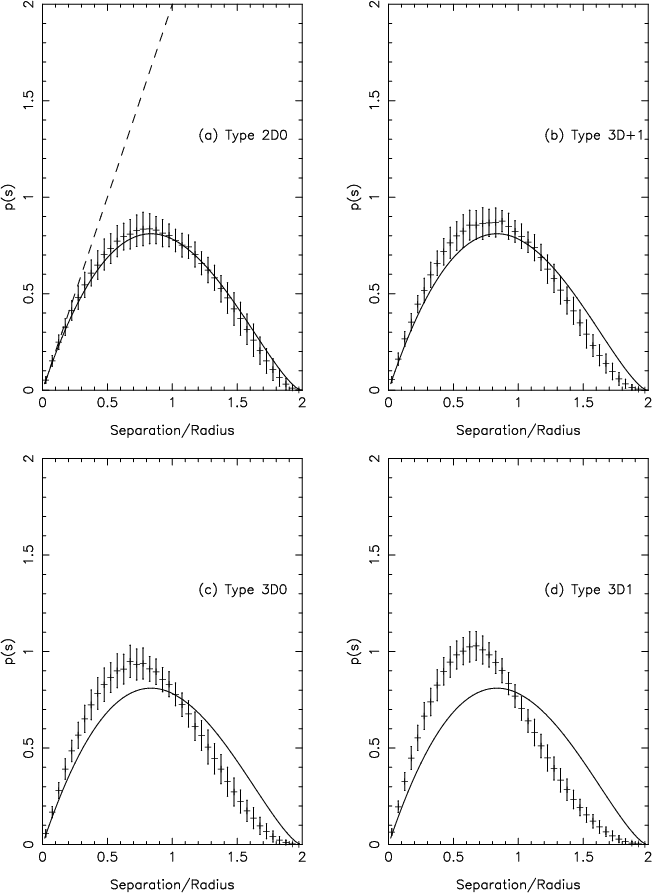 |
Figure 1:
Distribution function p(s) for separations between randomly
chosen stars in artificial (non-fractal) cluster of type
a) 2D0,
|
| Open with DEXTER | |
 |
Figure 2: Position data for the protostars referred to in the text. Top, RCW120, middle CN 138. Bottom the types I and II protostars from the W5 region. All the positions have been normalised by centreing on the mean position of the cluster members, and then setting the distance from the centre to the furthest star to be one distance unit. |
| Open with DEXTER | |
2 Methodology
Three different types of artificial star cluster were created, using
random numbers ![]() to generate the individual star positions. The first
type (2D0) is a circular cluster (i.e. two-dimensional disc) with statistically uniform surface density. This is the distribution expected from circular samples of randomly distributed data points. The second type (3D
to generate the individual star positions. The first
type (2D0) is a circular cluster (i.e. two-dimensional disc) with statistically uniform surface density. This is the distribution expected from circular samples of randomly distributed data points. The second type (3D![]() )
are spherical clusters (i.e. three-dimensional clusters)
with volume density
)
are spherical clusters (i.e. three-dimensional clusters)
with volume density
![]() and
and
![]() .
Thirdly a fractal or multiscale clustering is used to create clusters of type F(dim),
.
Thirdly a fractal or multiscale clustering is used to create clusters of type F(dim),
![]() .
dim indicates the Fractal Dimension, or space filling dimension, of the cluster, a value of 3.0 indicating homogeneous, unclustered space filling, and 1.5 the most sub-clustered distribution. All of the random artificial clusters are created with 100 to 300 stars. For a full description of the methods used for creating these clusters, see Cartwright & Whitworth (2004). For each type of cluster 1000 realisations are analysed, so that means and standard deviations
can be obtained for the parameters extracted. The three-dimensional clusters are projected onto an arbitrary plane
for analysis. The data for the real star clusters used are illustrated in Fig. 2 and the sources listed in Table 2.
.
dim indicates the Fractal Dimension, or space filling dimension, of the cluster, a value of 3.0 indicating homogeneous, unclustered space filling, and 1.5 the most sub-clustered distribution. All of the random artificial clusters are created with 100 to 300 stars. For a full description of the methods used for creating these clusters, see Cartwright & Whitworth (2004). For each type of cluster 1000 realisations are analysed, so that means and standard deviations
can be obtained for the parameters extracted. The three-dimensional clusters are projected onto an arbitrary plane
for analysis. The data for the real star clusters used are illustrated in Fig. 2 and the sources listed in Table 2.
Each cluster, real or artificial, is centred on the mean position of its stars, and distances are then normalised by setting the radius of the cluster (i.e. the distance from the mean of the stars' positions to the most distant star in the cluster) to unity. In the rest of this paper, all distances are normalised in this way.
3 The normalised correlation length
The normalised correlation length, also known as the ``first moment'', is a
single measurement characteristic of the distribution function p(s), where
![]() gives the probability that the projected separation between two cluster
stars chosen at random is in the interval
gives the probability that the projected separation between two cluster
stars chosen at random is in the interval
![]() .
To obtain p(s)
empirically, we define
.
To obtain p(s)
empirically, we define
![]() equal bins in the range
equal bins in the range
![]() ,
so all the bins have width
,
so all the bins have width
![]() .
Thus the ith bin corresponds to the interval
.
Thus the ith bin corresponds to the interval
![]() ,
and to the mean value
,
and to the mean value
![]() .
Then we count the number of separations
.
Then we count the number of separations
![]() falling
in each bin, and put
falling
in each bin, and put
| (1) |
where
Figure 1a presents the results obtained from 1000
clusters of type 2D0, a disc with uniform surface-density. The
plotted points give the mean
![]() from the 1000 realizations,
and the error bars give the width of the bin and the
from the 1000 realizations,
and the error bars give the width of the bin and the ![]() standard deviation. If there were no edge effects (i.e. if the uniform
surface-density extended to infinity in two dimensions), we would
have
p(s) = 2 s, and this is indeed a good fit to
standard deviation. If there were no edge effects (i.e. if the uniform
surface-density extended to infinity in two dimensions), we would
have
p(s) = 2 s, and this is indeed a good fit to
![]() at
small s values, as indicated by the dashed line in Fig. 1a.
at
small s values, as indicated by the dashed line in Fig. 1a.
For a circle of unit radius populated with complete spatial randomness,
p(s) is given by (Diggle 2003):
![\begin{displaymath}{p(s)\!=\! 1\!+\!\frac{1}{\pi}\!\left[2(s^2\!-\!1)\cos^{-1}(s/2)\!-s(1\!+\!s^2\!/2)\sqrt(1\!-\!s^2/4)\right]}
\end{displaymath}](/articles/aa/full_html/2009/33/aa12331-09/img30.png)
for all
The solid line in Fig. 1a shows that this function fits the plotted points well, and it is included in all the other plots for reference, i.e. to emphasize the differences between the distributions.
The overall structure of the cluster is well represented by p(s), as
can be seen from Figs. 1b through 1d,
which show the results obtained for three other types of artificial star cluster.
Figure 1c shows how p(s)
is slewed towards smaller s values for a projected sphere with constant density. This is due to the
extra depth, and therefore larger number of stars, in the central region of the projected cluster, which
results in more small separations between stars.
This bias towards shorter separations is even more pronounced for Fig. 1d,
a projected sphere with a centrally concentrated density,
![]() .
.
Table 1: Clustering measures obtained for artificial star clusters.
Figure 1b gives p(s) for a sphere with density which increases with
radius,
![]() .
It can be seen that p(s) for this configuration lies
somewhere between those shown in Figs. 1a and 1c. By comparison,
p(s) for a sphere with multiscale subclustering shows many peaks, corresponding to the distances
between subclusters and the mean distances within them (Fig. 2 in Cartwright & Whitworth 2004).
.
It can be seen that p(s) for this configuration lies
somewhere between those shown in Figs. 1a and 1c. By comparison,
p(s) for a sphere with multiscale subclustering shows many peaks, corresponding to the distances
between subclusters and the mean distances within them (Fig. 2 in Cartwright & Whitworth 2004).
The Normalized Correlation Length is the mean separation ![]() between stars in
a cluster, and is therefore the mean value of the distributions in Fig. 1.
Table 1 gives mean values of
between stars in
a cluster, and is therefore the mean value of the distributions in Fig. 1.
Table 1 gives mean values of ![]() and their standard deviations, for the
artificial cluster types tested. It can be seen that increasing values of
and their standard deviations, for the
artificial cluster types tested. It can be seen that increasing values of
![]() are measured for anticlustered data, while
are measured for anticlustered data, while
![]() is monotonically decreasing for clustered data, whether radially or fractally clustered.
is monotonically decreasing for clustered data, whether radially or fractally clustered.
In order to test the robustness of ![]() with varying numbers of stars in the clusters, means and standard deviations were calculated for 1000 examples of each cluster type with 85, 100, 300 and 500 members. The results are in Table A.2 in the Appendix.
with varying numbers of stars in the clusters, means and standard deviations were calculated for 1000 examples of each cluster type with 85, 100, 300 and 500 members. The results are in Table A.2 in the Appendix.
Additionally, clusters of 1000 members were created and then 100 different subsamples of 200 members were randomly selected and analysised to produce ![]() .
The results are in Table A.1 in the appendix. This table also shows the variation in the calculated centre (mean position) of the cluster, depending on which stars are selected from a cluster. Column 1 lists the cluster type and Col. 2 the mean and standard deviation of
.
The results are in Table A.1 in the appendix. This table also shows the variation in the calculated centre (mean position) of the cluster, depending on which stars are selected from a cluster. Column 1 lists the cluster type and Col. 2 the mean and standard deviation of ![]() .
Columns 3 and 4 give the mean and standard deviation of the mean position of the cluster, in units of the radius of the original spherical distribution of points.
.
Columns 3 and 4 give the mean and standard deviation of the mean position of the cluster, in units of the radius of the original spherical distribution of points.
4 Results
Table 1 shows that ![]() decreases monotonically as distributions become more clustered, whether radially or multiscale, and increases monotonically as they become radially anticlustered. A value of s=0.8 corresponds to a statistically uniform density. (In the limit, numerical investigations revealed that
decreases monotonically as distributions become more clustered, whether radially or multiscale, and increases monotonically as they become radially anticlustered. A value of s=0.8 corresponds to a statistically uniform density. (In the limit, numerical investigations revealed that ![]() reaches a maximum value of 1.17 for a ring of stars viewed face on.)
reaches a maximum value of 1.17 for a ring of stars viewed face on.) ![]() can therefore be used to distinguish between clustered and anticlustered distributions. Tests also confirm the robustness of
can therefore be used to distinguish between clustered and anticlustered distributions. Tests also confirm the robustness of ![]() and its invariance with number of stars in a cluster and the selection or omission of points within the sample (Tables A.2 and A.1).
and its invariance with number of stars in a cluster and the selection or omission of points within the sample (Tables A.2 and A.1).
Table 1 also lists the mean edge length m of the minimal spanning tree and the derived
![]() for each cluster. Cartwright & Whitworth (2004) showed that Q can be used to distinguish the two types of clustering, radial and multiscale, and indeed this can be seen in the table, Q>0.8 indicating fractal-type, multiscale clustering, and Q<0.8 indicating radial clustering. However, the anticlustered data also yield a Q<0.8, and so a simple measurement of Q does not distinguish fractal sub-clustering and anticlustering.
for each cluster. Cartwright & Whitworth (2004) showed that Q can be used to distinguish the two types of clustering, radial and multiscale, and indeed this can be seen in the table, Q>0.8 indicating fractal-type, multiscale clustering, and Q<0.8 indicating radial clustering. However, the anticlustered data also yield a Q<0.8, and so a simple measurement of Q does not distinguish fractal sub-clustering and anticlustering.
Table 2: Real star clusters.
The confusion is avoided by first using s to distinguish between clustered and anti-clustered data, and then applying Q for data which is apparently clustered, to establish whether the clustering is radial or multiscale.
Table 2 reports the value of ![]() obtained for young stars in the RCW 120 and CN 138 regions, as reported by Deharveng et al. (2009) and Watson et al. (2009). A value of 0.67 for
obtained for young stars in the RCW 120 and CN 138 regions, as reported by Deharveng et al. (2009) and Watson et al. (2009). A value of 0.67 for ![]() for RCW120 does not indicate anticlustering. However, a value of 0.84 for the CN 138 region does indicate anticlustering.
for RCW120 does not indicate anticlustering. However, a value of 0.84 for the CN 138 region does indicate anticlustering.
The values of ![]() for clustered, anti clustered and statistically random distributions are very close. A statistical test is therefore performed in order to establish the probability of obtaining a value of
for clustered, anti clustered and statistically random distributions are very close. A statistical test is therefore performed in order to establish the probability of obtaining a value of
![]() from a random or fractally clustered distribution, and compare this with the probability of obtaining it from an anticlustered distribution. The test is performed as follows. First we wish to reject the hypothesis that the observed data are randomly arranged, either in 2 or 3 dimensions. 1000 simulations are performed using the 3D0 cluster type, with the same number of points as CN 138 (85) yielding 1000 values of
from a random or fractally clustered distribution, and compare this with the probability of obtaining it from an anticlustered distribution. The test is performed as follows. First we wish to reject the hypothesis that the observed data are randomly arranged, either in 2 or 3 dimensions. 1000 simulations are performed using the 3D0 cluster type, with the same number of points as CN 138 (85) yielding 1000 values of ![]() .
These are placed in size order, and compared with the value obtained for the CN 138 data. As each value of
.
These are placed in size order, and compared with the value obtained for the CN 138 data. As each value of ![]() has equal probability, the position of the observed value of
has equal probability, the position of the observed value of ![]() in the ordered set of random observations indicates the probability that a value greater than or equal to the observed value can be obtained from a 3D0 type cluster (see e.g. Diggle 2003). Out of 1000 simulations of the 3D0 clusters, only 60 yielded
in the ordered set of random observations indicates the probability that a value greater than or equal to the observed value can be obtained from a 3D0 type cluster (see e.g. Diggle 2003). Out of 1000 simulations of the 3D0 clusters, only 60 yielded
![]() ,
giving a confidence level of
,
giving a confidence level of ![]() that the 3D0 hypothesis can be rejected. Similarly, the 2D0 hypothesis, that the stars are randomly arranged in 2 dimensions, and the Fractal hypothesis, that CN 138 is fractally clustered with a dimension of D=2.5, may be rejected with
that the 3D0 hypothesis can be rejected. Similarly, the 2D0 hypothesis, that the stars are randomly arranged in 2 dimensions, and the Fractal hypothesis, that CN 138 is fractally clustered with a dimension of D=2.5, may be rejected with ![]() confidence. The values of
confidence. The values of ![]() for radial density gradients proportional to r and r1.5 are closest to the measured value for CN 138. Therefore, on the basis of the measured value of
for radial density gradients proportional to r and r1.5 are closest to the measured value for CN 138. Therefore, on the basis of the measured value of ![]() ,
the protostars in the
CN 138 region are found to be anticlustered with a density proportional to
,
the protostars in the
CN 138 region are found to be anticlustered with a density proportional to
![]() where
where
![]() .
.
5 Discussion
Tests on artificial star clusters show that the correlation length
If the mean edge length of the mimimal spanning tree m is also calculated, and used to obtain
![]() ,
then
,
then ![]() permits the two types of clustering to be distinguished. However, Table 2 shows that confusion may arise if
permits the two types of clustering to be distinguished. However, Table 2 shows that confusion may arise if ![]() is calculated for a distribution which is anticlustered, as the
is calculated for a distribution which is anticlustered, as the ![]() value is likely to be less than 0.8, falsely indicating a fractally subclustered distribution. It is important therefore, that users of
value is likely to be less than 0.8, falsely indicating a fractally subclustered distribution. It is important therefore, that users of ![]() check the value of
check the value of ![]() before proceeding to the calculation and interpretation of
before proceeding to the calculation and interpretation of ![]() .
.
The fact that the correlation length s of a cluster can indicate a region of anticlustering is in itself a useful tool. The formation of stars produces stellar winds and ionizing radiation which are predicted to disrupt the surrounding molecular clouds, triggering further star formation. Elmegreen & Lada (1977) proposed the collect and collapse mechanism, whereby expanding HII regions would sweep up spherical shells of matter from the inter-stellar medium, which would then collapse to form stars. Recent work has identified such bubbles, together with accurate census data of their associated star forming regions (Koenig et al. 2008; Deharveng et al. 2009; Watson et al. 2009). If the collect and collapse mechanism occurs in nature, one would expect the spatial distribution of the observed stars to bear the imprint of this process. The star formation rate should increase with the distance away from the centre of the expanding bubble, and should therefore be radially anticlustered.
Tests on observations of protostars which are believed to be forming in an expanding HII region,
and therefore may be anticlustered, produce mixed results. Data from the CN 138 region (Watson et al. 2009) do show an increased ![]() ,
consistent with anticlustering, and a density gradient proportional to
,
consistent with anticlustering, and a density gradient proportional to
![]() where
where
![]() .
The possibility of a random arrangement of stars producing this value of
.
The possibility of a random arrangement of stars producing this value of ![]() can be ruled out with 94
can be ruled out with 94![]() confidence. Data from the RCW120 region (Deharveng et al. 2009), however, give a lower value of
confidence. Data from the RCW120 region (Deharveng et al. 2009), however, give a lower value of ![]() ,
consistent with clustering. In this case, it can be seen from Fig. 2 that there are several small clusters in the data, and the existence of these small clusters would tend to reduce
,
consistent with clustering. In this case, it can be seen from Fig. 2 that there are several small clusters in the data, and the existence of these small clusters would tend to reduce ![]() cancelling out the signature of the radial anticlustering.
cancelling out the signature of the radial anticlustering.
Koenig et al. (2008) have also published observations of protostars forming in association with expanding HII bubbles, and these form arcs and ``elephants'' trunks' which are very suggestive of triggered star formation. ![]() would not be able to diagnose anticlustering in this situation, as the arcs do not form complete circles.
would not be able to diagnose anticlustering in this situation, as the arcs do not form complete circles. ![]() is only able to detect anticlustering when the stars are forming in a fairly homogeneous arrangement, and when there are no tight knots of stars.
is only able to detect anticlustering when the stars are forming in a fairly homogeneous arrangement, and when there are no tight knots of stars.
It should also be noted that a random arrangement of stars in two dimensions, or cluster type 2D0, will also give increased values of ![]() .
It is therefore necessary to ensure that observational criteria are used to include only the stars in the three dimensional volume of interest, before applying the correlation length analysis.
.
It is therefore necessary to ensure that observational criteria are used to include only the stars in the three dimensional volume of interest, before applying the correlation length analysis.
6 Conclusion
Users of the
![]() parameter should ensure that they calculate the correlation length
parameter should ensure that they calculate the correlation length ![]() first, and exclude the possibility of anticlustered data, before proceeding to the calculation of
first, and exclude the possibility of anticlustered data, before proceeding to the calculation of ![]() and its interpretation.
The correlation length
and its interpretation.
The correlation length ![]() increases monotonically as clusters are more radially anticlustered.
increases monotonically as clusters are more radially anticlustered. ![]() can therefore be used to estimate the radial density gradient of star clusters whether the gradient is positive or negative. It can also be used to rule out spatial randomness. The technique fails if the region being studied has subclusters of stars, or if only a part of a spherical bubble of stars exists.
can therefore be used to estimate the radial density gradient of star clusters whether the gradient is positive or negative. It can also be used to rule out spatial randomness. The technique fails if the region being studied has subclusters of stars, or if only a part of a spherical bubble of stars exists.
Acknowledgements
The author is a Royal Society Dorothy Hodgkin Research Fellow. Thanks to C. Watson and L. Deharveng for providing early access to their data, and to the anonymous referee for helpful comments and questions.
Appendix A: Stability tests on

Table A.1:
Variance of ![]() and calculated centre (mean position) of cluster, when calculated from subsets
of 200 points randomly selected from 1000 cluster members.
and calculated centre (mean position) of cluster, when calculated from subsets
of 200 points randomly selected from 1000 cluster members.
Table A.2:
Variance of
![]() with numbers of objects in cluster.
with numbers of objects in cluster.References
All Tables
Table 1: Clustering measures obtained for artificial star clusters.
Table 2: Real star clusters.
Table A.1:
Variance of ![]() and calculated centre (mean position) of cluster, when calculated from subsets
of 200 points randomly selected from 1000 cluster members.
and calculated centre (mean position) of cluster, when calculated from subsets
of 200 points randomly selected from 1000 cluster members.
Table A.2:
Variance of ![]() with numbers of objects in cluster.
with numbers of objects in cluster.
All Figures
| |
Figure 1:
Distribution function p(s) for separations between randomly
chosen stars in artificial (non-fractal) cluster of type
a) 2D0,
|
| Open with DEXTER | |
| In the text | |
| |
Figure 2: Position data for the protostars referred to in the text. Top, RCW120, middle CN 138. Bottom the types I and II protostars from the W5 region. All the positions have been normalised by centreing on the mean position of the cluster members, and then setting the distance from the centre to the furthest star to be one distance unit. |
| Open with DEXTER | |
| In the text | |
Copyright ESO 2009
Current usage metrics show cumulative count of Article Views (full-text article views including HTML views, PDF and ePub downloads, according to the available data) and Abstracts Views on Vision4Press platform.
Data correspond to usage on the plateform after 2015. The current usage metrics is available 48-96 hours after online publication and is updated daily on week days.
Initial download of the metrics may take a while.