| Issue |
A&A
Volume 503, Number 2, August IV 2009
|
|
|---|---|---|
| Page(s) | 589 - 590 | |
| Section | The Sun | |
| DOI | https://doi.org/10.1051/0004-6361/20079221e | |
| Published online | 09 July 2009 | |
Erratum
Drift instabilities in the solar corona within the multi-fluid description
R. Mecheri 1 - E. Marsch2
1 - Queen Mary University of London, Astronomy Unit,
Mile End Road, E1 4NS, London, UK
2 -
Max-Planck institut für Sonnensystemforschung,
Max-Planck Strasse 2, 37191 Katlenburg-Lindau, Germany
A&A 481, 853-860 (2008), DOI: 10.1051/0004-6361:20079221
The purpose of this erratum is to point out and to correct
some unfortunate typographical mistakes, as well as algebraic errors
contained in our paper ``Drift instabilities in
the solar corona within the multi-fluid description'' published in A&A 481, 853 (2008). We also want to
clarify some important issues with respect to the assumed background
state on which the drift-wave instability develops.
The first point is that the nonuniformity of the background density
in the corona model considered should be expressed more precisely as
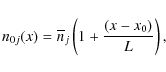 |
(1) |
whereby the density increases linearly in the coordinate x with respect to some arbitrary reference location x0, at which the density is assumed to have the constant value
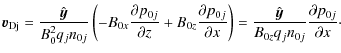
Also, the expression of the drift velocity should not contain the
factor
![]() since we assumed an ideal gas law
since we assumed an ideal gas law
![]() with
with
![]() the mass density. Consequently, the acoustic speed
Csj is given by
the mass density. Consequently, the acoustic speed
Csj is given by
![]() ,
and not
,
and not
![]() as quoted in the original paper. Thus the correct expression of the
drift velocity is
as quoted in the original paper. Thus the correct expression of the
drift velocity is
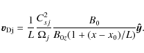 |
(2) |
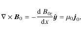
The second major issue is related to the properties of the assumed background plasma state in the paper by Mecheri & Marsch (2008). If the background electric field
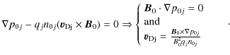 |
(3) |
Thus in equilibrium the background pressure (and density) gradient must be across
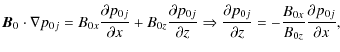 |
and then from (3) we have
 |
Thus, the insertion of the expression for
However, because of the equilibrium diamagnetic current density in
the y-direction,
![]() ,
the background magnetic field must also be
perturbed according to Ampère's law. This subtle issue has not
been investigated and discussed in the original paper, in which it
was assumed (but not mentioned explicitly) that the field
perturbation should be negligible due to the low beta of the coronal
plasma, where the magnetic pressure dominates the gas pressure. To
clarify this point, we now investigate the corresponding equation.
For simplicity, we consider that the background plasma has a
magnetic field
,
the background magnetic field must also be
perturbed according to Ampère's law. This subtle issue has not
been investigated and discussed in the original paper, in which it
was assumed (but not mentioned explicitly) that the field
perturbation should be negligible due to the low beta of the coronal
plasma, where the magnetic pressure dominates the gas pressure. To
clarify this point, we now investigate the corresponding equation.
For simplicity, we consider that the background plasma has a
magnetic field
![]() with only one component in the
z-direction and a density and pressure gradient in the
x-direction. Thus for the curl of
with only one component in the
z-direction and a density and pressure gradient in the
x-direction. Thus for the curl of
![]() ,
Ampère's law
gives
,
Ampère's law
gives
 |
(4) |
which by use of (3) can in turn be written as total pressure equilibrium in the form:
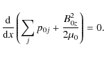 |
(5) |
Integration of Eq. (5) with respect to the reference position x0, which has a reference field strength
| (6) |
It can be clearly seen that, for small plasma beta
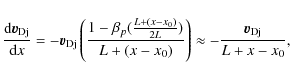 |
(7) |
where we have used
| (8) |
which agrees with the approximations adopted in our paper, in the sense that the wavelength of interest,
In conclusion, it turns out that the only difference with the original equations of the paper by Mecheri & Marsch (2008) is the missing term (1+(x-x0)/L)-1 in their expression for the drift velocity. This does not affect the result concerning the local perturbation analysis, since those were calculated at the reference location x0, where (1+(x-x0)/L)-1=1. These results were in turn used as initial conditions to solve the ray-tracing equations (as mentioned in Sect. 3.3 of the original paper). However, the results concerning the nonlocal (i.e., ray-tracing) analysis should be recalculated, since (1+(x-x0)/L)-1 is no longer equal to the unity when moving away from the reference location x0.
The ray-tracing recalculation should also take into account an
additional variation of the background pressure (and density) in the
z-direction, in order to consistently fulfill the equilibrium
conditions (3) mentioned previously. Such a variation may also be
represented by a linear profile (similar to the one in the
x-direction). In this case the results of the local perturbation
analysis will again remain unchanged; however, the extent of the
region for which the new ray-tracing calculations are to be
performed must be restricted to a smaller region (of ![]() 10 km),
thus satisfying that the density is allowed to increase locally by
at most a factor
10 km),
thus satisfying that the density is allowed to increase locally by
at most a factor ![]() 10 (as mentioned at the end of Sect. 2 of
the original paper). Considering this will prevent an increase in
the density to unrealistically high coronal values. All this
unfortunately was not adequately considered in the original paper.
10 (as mentioned at the end of Sect. 2 of
the original paper). Considering this will prevent an increase in
the density to unrealistically high coronal values. All this
unfortunately was not adequately considered in the original paper.
Acknowledgements
We thank an unknown referee for his considerable efforts in reviewing our original paper with respect to these critical issues, and we appreciate his valuable comments that stimulated and greatly contributed to this erratum.
References
- Mecheri, R., & Marsch, E. 2008, A&A, 481, 853 [NASA ADS] [CrossRef] [EDP Sciences] (In the text)
Copyright ESO 2009
Current usage metrics show cumulative count of Article Views (full-text article views including HTML views, PDF and ePub downloads, according to the available data) and Abstracts Views on Vision4Press platform.
Data correspond to usage on the plateform after 2015. The current usage metrics is available 48-96 hours after online publication and is updated daily on week days.
Initial download of the metrics may take a while.