| Issue |
A&A
Volume 503, Number 2, August IV 2009
|
|
|---|---|---|
| Page(s) | 373 - 378 | |
| Section | Cosmology (including clusters of galaxies) | |
| DOI | https://doi.org/10.1051/0004-6361/200912492 | |
| Published online | 02 July 2009 | |
Non-Maxwellian electron distributions in clusters of galaxies
J. S. Kaastra1,2 - A. M. Bykov3 - N. Werner4
1 - SRON Netherlands Institute for Space Research, Sorbonnelaan 2, 3584 CA Utrecht, The Netherlands
2 - Sterrenkundig Instituut, Universiteit Utrecht, PO Box 80000, 3508 TA Utrecht, The Netherlands
3 - A.F. Ioffe Institute of Physics and
Technology, St. Petersburg 194021, Russia
4 - Kavli Institute for Particle Astrophysics and Cosmology,
Stanford University, 452 Lomita Mall/mc 4085, Stanford, CA 94305, USA
Received 14 May 2009 / Accepted 28 May 2009
Abstract
Context. Thermal X-ray spectra of clusters of galaxies and other sources are commonly calculated assuming Maxwellian electron distributions. There are situations where this approximation is not valid, for instance near interfaces of hot and cold gas and near shocks.
Aims. The presence of non-thermal electrons affects the X-ray spectrum. To study the role of these electrons in clusters and other environments, an efficient algorithm is needed to calculate the X-ray spectra.
Methods. We approximate an arbitrary electron distribution by the sum of Maxwellian components. The decomposition uses either a genetic algorithm or an analytical approximation. The X-ray spectrum is then evaluated with a linear combination of those Maxwellian components.
Results. Our method is fast and leads to an accurate evaluation of the spectrum. The Maxwellian components allow the use of the standard collisional rates that are available in plasma codes such as SPEX. We give an example of a spectrum for the supra-thermal electron distribution behind a shock in a cluster of galaxies. The relative intensities of the satellite lines in such a spectrum are sensitive to supra-thermal electrons. These lines can only be investigated with high spectral resolution. We show that the instruments on future missions like Astro-H and IXO will be able to demonstrate the presence or absence of these supra-thermal electrons.
Key words: acceleration of particles - radiation mechanisms: general - X-rays: galaxies: clusters - X-rays: general
1 Introduction
Most of the visible baryonic matter in clusters of galaxies is in the form of a hot, tenuous gas. Usually it is assumed that this gas is in collisional ionisation equilibrium. In the central parts, the density is high enough and the timescales long enough to fulfil the conditions for collisional ionisation equilibrium. In the outer parts this may not always be the case. Freshly accreted gas may still be ionising. For a review of equilibration processes in such tenuous plasmas, see Bykov et al. (2008). Nevertheless, usually a Maxwellian electron distribution is still assumed to be valid; however, there are situations where this is not an obvious constraint. For instance, in cooling cores of clusters, electrons from hot gas may penetrate the colder parts. Also, when shocks are present, deviations from a Maxwellian distribution may occur associated with the temperature gradients or caused by particles accelerated by the shock. Shocks can stem from merger activity, AGN jets, and accretion shocks may occur in cluster outskirts. As the Coulomb thermal relaxation times increases with electron energy E as E3/2, supra-thermal electrons are relatively long-lived and may yield a pressure contribution that is potentially interesting for mass profiles. The presence of such supra-thermal electrons can be revealed by excess emission in satellite lines.
In this paper we describe a way to model the emerging X-ray emission spectra for the case of a non-Maxwellian electron distribution. Although our main focus here is on clusters of galaxies, the same procedure can be applied to different circumstances, for instance in stellar coronae, supernova remnants, and the Galactic ridge; for the last case see also Masai et al. (2002) and Tatischeff (2003).
2 X-ray spectra for supra-thermal electron distributions
To calculate an X-ray spectrum, essentially two steps are needed: 1) determine the ionisation balance and; 2) calculate the corresponding spectrum. For more details see e.g. Kaastra et al. (2008).
We first consider the ionisation balance. To determine that, it is necessary to evaluate the collisional ionisation and recombination rates for all ions. These rates are derived by integrating the relevant cross sections over the electron distribution. For instance, the collisional ionisation rate
![]() is given by
is given by
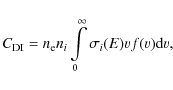
where ne and ni are the densities of electrons and the ion i considered,
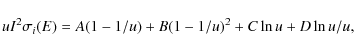
In the most simple approximation, the cross section for collisional ionisation can be written as (Lotz 1967):
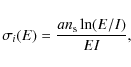
where E is the kinetic energy of the free electron, ns is the number of electrons in a given atomic shell and the normalisation
with
A similar treatment can be made for other relevant rates, like the collisional
excitation rates that are important for the line emission. However, some rates
cannot be written in a form that allows analytical integration over a Maxwellian electron distribution. A good example are the radiative recombination rates. We recall that the cross section for radiative recombination
![]() can be expressed in terms of the photoionisation cross section through Milne's relation as
can be expressed in terms of the photoionisation cross section through Milne's relation as
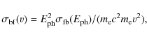
where
It is clear that we need to follow an alternative approach for non-Maxwellian
electron distributions. There have been attempts to make a generalisation of the
Maxwell distribution. For instance, Porquet et al. (2001) combine a Maxwellian at
low energies with a power-law at high energies, but they only consider the
ionisation balance, not the resulting spectrum. Prokhorov et al. (2009) adopt a
similar approximation for the electron distribution, but only consider continuum
emission and the Fe XXV and Fe XXVI 1s-2p blends.
Owocki & Scudder (1983) use the so-called kappa-distribution (Olbert et al. 1967):
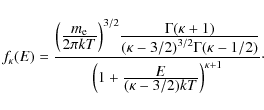
This distribution tends to a Maxwellian for
3 The multi-Maxwellian approach
Plasma codes generally may contain (ten)thousands of spectral lines, and at high spectral resolution, spectra contain many bins. Therefore, numerical integration for each rate over the electron distribution is a very time consuming task, and not of practical use, in particular when spectral fitting is performed and the model needs to be evaluated many times.
But all relevant rates in the case of the collisionally ionised plasmas that we
consider here, are proportional to the product
neni, as
for each of these rates the interaction (collision) of an electron with an ion
is the driving process. Therefore, all rates are linearly proportional to the
electron density
ne. If we decompose the electron distribution into
a linear combination of elementary components, the total rate for any process is
simply the sum of the rates for these individual elementary components. Now, for
Maxwellian electron distributions all rates are well known and fast to evaluate
analytically or with analytical approximations. Thus, if we decompose an
arbitrary electron distribution f(E) into a linear combination of Maxwellians:
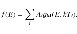
with Ai the normalisation constant for component i and gM(E,Ti) the Maxwell distribution for temperature Ti, then the calculation of any rate (recombination, ionisation, excitation) is simple and straightforward. The problem is then reduced to obtaining the normalisations Ai and temperatures Ti for an arbitrary electron distribution f(E).
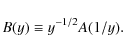
In principle, one might solve formally the integral equation
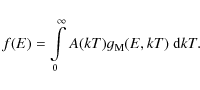
Using
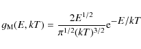
(7) can be cast into the shape of a Laplace transform as
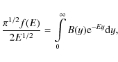
with
 |
(10) |
The calculation of the inverse Laplace transform is not always trivial. For instance, when we consider a mono-energetic beam, f(E) is essentially a delta-function, and the formal solution is a sine-wave with infinite frequency, which is not very practical. Fortunately, in most practical cases f(E) is a smooth function of energy, spanning a broad range of energies.
There are various ways to solve (9). There is software available that can do the inverse Laplace transform numerically (for example d'Amore et al. 1999), but in practice this is difficult, because these algorithms only work if the left-hand-side of (9) is an analytical function. However, in practice the electron distributions are given in tabular form, and the algorithms used to interpolate such tables do not produce a formal analytical function (the requirement that the function is infinitely differentiable is usually violated). There are two solutions to this problem that we elaborate in the next subsections: direct approximation of the electron distribution by an analytical function, or direct decomposition of the electron distribution as a sum of Maxwellians.
3.1 Approximation of the electron distribution by an analytical function
In practice, apart from the most pathological cases, electron distributions contain a core that is close to Maxwellian, plus a high energy tail. For an example see Sect. 4. After some experimentation, we found
that the electron distribution of that example can be approximated by the following series:
![\begin{displaymath}f(E) = \frac{x}{2kT_0} \Bigl[ c_0 {\rm e}^{\displaystyle{-a_0...
...}
+ \sum\limits_{k=1}^4 \frac{c_k}{(a_k+x^2)^{2+k/2}} \Bigr],
\end{displaymath}](/articles/aa/full_html/2009/32/aa12492-09/img23.png)
with x the dimensionless momentum defined by
 |
(12) |
and where T0 is a characteristic temperature corresponding to the electron distribution, and the parameters ck and ak can be adjusted to give the best fit.
Equation (11) is an analytical function, and the inverse Laplace
transform in this case can be done analytically, yielding
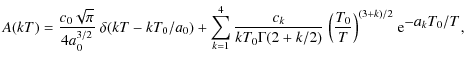
where
For our example, the normalisations c0-c4 are 0.755, 0.0609, 2.54, 13.3, and 17.58, respectively; the scale factors a0-a4 are 0.483, 152, 6843, 57.4 and 12.4. The fit is not perfect, but better than 0.5% for x<30, and better than 1% for x<700. The relative difference to the exact distribution are shown in Fig. 2.
3.2 Direct decomposition of the electron distributions as the sum of Maxwellians
We seek an approximation to f(E) that can be written as a linear combination of n Maxwellians, with n a given number. The solution can be represented as
a set of pairs (Ti,Ai) with Ti the temperatures and Ai the normalisations. We will choose for convenience a set of increasing temperatures
(
Ti+1>Ti), and we will demand that ![]() (physically allowed components). Most realistic electron distributions can be represented as a Maxwellian with high-energy tails. Therefore, the first temperature T1 should be close to the temperature T0 of this dominant Maxwellian component.
(physically allowed components). Most realistic electron distributions can be represented as a Maxwellian with high-energy tails. Therefore, the first temperature T1 should be close to the temperature T0 of this dominant Maxwellian component.
This then leads to the following approach. We define a set of nlogarithmically spaced temperature intervals
(T1,i,T2,i) with T1,1 equal to T0 and for all i, we take
T2,i=sT1,i and
T1,i=T2,i-1. For the parameter s>1 we adopt a value of 1.5. The total
temperature range spanned by these n contiguous intervals is therefore
T0 - sn T0. For each interval, we choose an arbitrary temperature Ti within this interval (
![]() )
and an arbitrary normalisation
)
and an arbitrary normalisation ![]() .
We scale the Ai in such a way that their sum corresponds to the total electron density. We then check how close the resulting electron distribution is to the electron distribution f(E) that we want to approximate. By varying all values Ti within their allowed ranges (the above mentioned intervals) and also the values for Ai, we try to get the best possible approximation.
.
We scale the Ai in such a way that their sum corresponds to the total electron density. We then check how close the resulting electron distribution is to the electron distribution f(E) that we want to approximate. By varying all values Ti within their allowed ranges (the above mentioned intervals) and also the values for Ai, we try to get the best possible approximation.
We use the genetic algorithm PIKAIA developed by Charbonneau (1995) to find the best solution. This algorithm needs a formal function of the parameters (Ti, Ai) that needs to be maximised. For this function we choose the inverse of the sum of the squared relative deviations of the approximation to the true electron distribution f(E).
After some experimenting, we obtained satisfactory convergence with the following initial parameters: number of individuals 500, number of generations 500. All other parameters in PIKAIA were kept to their default values. The number of individuals represents here the number of sets (Ti,Ai) from which the iteration starts; the number of generations is the number of iterations during which the individual sets evolve towards the optimum solution.
We have tested our algorithm on various different electron distributions, but give here only one illustrative example.
4 Example of decomposition of an electron distribution into Maxwellians
![\begin{figure}
\par\resizebox{9cm}{!}{\includegraphics[angle=-90]{12492f1.ps}}
\end{figure}](/articles/aa/full_html/2009/32/aa12492-09/img31.png) |
Figure 1: Electron distributions immediately after a shock with different Mach numbers, in the downstream region. The distributions are expressed here in terms of the dimensionless momentum (normalised to the thermal momentum in the far upstream region). The distributions are normalised to integral unity. Solid line: M = 2.2; dashed line: M=1.5; dash-dotted line: M=1.2; dotted line: far upstream Maxwellian distribution. |
| Open with DEXTER | |
![\begin{figure}
\par\resizebox{9cm}{!}{\includegraphics[angle=-90]{12492f2.ps}}
\end{figure}](/articles/aa/full_html/2009/32/aa12492-09/img32.png) |
Figure 2: Relative differences of approximations to the electron distribution with M = 2.2 of Fig. 1. Upper panel: analytical approximation (11), see Sect. 3.1; lower panel: approximation using the sum of 32 Maxwellian components, see Sect. 3.2. |
| Open with DEXTER | |
![\begin{figure}
\par\resizebox{9cm}{!}{\includegraphics[angle=-90]{12492f3.ps}}
\end{figure}](/articles/aa/full_html/2009/32/aa12492-09/img33.png) |
Figure 3: Relative normalisations versus temperature for the 32 Maxwellian components used in the approximation of the electron distribution that is shown in Fig. 2. Histogram: the analytical approximation (13); Dots: the solution from the genetic algorithm. |
| Open with DEXTER | |
We have used electron distributions based on the models of Bykov & Uvarov (1999) for collisionless MHD shocks taking into account particle acceleration and a shock precursor. We consider here a case for a pre-shock temperature of T0=108 K, electron density 103 m-3, magnetic field 10-10 T, and shock size 100 kpc. In the simulation we assumed a pure Maxwellian distribution of electrons in the far upstream region of the flow and thus only the direct injection of electrons from the upstream thermal pool to Fermi type shock acceleration is responsible for the non-thermal electron population. The electron distribution in the immediate post-shock region is shown in Fig. 1 for three different Mach numbers. The model distribution was calculated taking account of both Fermi-type acceleration in a collisionless shock and Coulomb losses of the electrons in both the upstream and downstream regions. It is normalised to the momentum p0 corresponding to the typical energy kT0. Note that the supra-thermal electron distribution well away from the shock front differs from that shown in Fig. 1, because the efficient Coulomb losses wash-out the non-relativistic supra-thermal electrons.
There is a variant of the model where mildly relativistic electrons (with Lorentz factors ![]() 30) comprising a putative long-lived cosmic ray electron population in the ICM are re-accelerated by the MHD-shocks. The energy
efficiency problem is alleviated in that model in comparison with the case of only direct particle injection from the thermal plasma. However, in this paper we concentrate mostly on the diagnostic of non-relativistic electrons and thus
we consider only a direct injection model.
30) comprising a putative long-lived cosmic ray electron population in the ICM are re-accelerated by the MHD-shocks. The energy
efficiency problem is alleviated in that model in comparison with the case of only direct particle injection from the thermal plasma. However, in this paper we concentrate mostly on the diagnostic of non-relativistic electrons and thus
we consider only a direct injection model.
For our example, we take the case of M=2.2. In our decomposition with the genetic algorithm we have taken n=32 Maxwellians. The relative differences of the approximation compared to the exact electron distribution is shown in Fig. 2. The temperatures and relative normalisations of the solution are shown in Fig. 3. We have also used the analytical approximation (13) and binned it into similar temperature bins as the solutions from the genetic algorithm.
5 Spectrum for the supra-thermal electron distribution
We have adjusted all models in the spectral fitting package SPEX that involve emission or absorption from a hot plasma. All these models now include an option to account for supra-thermal electrons. They have an additional parameter, which is the name of a file containing the temperatures and relative emission measures of the Maxwellian components. As SPEX does not use pre-calculated tables but calculates spectra on the fly, all relevant rates (ionisation, recombination, excitation) are simply calculated by adding the contributions from the Maxwellian components. Obviously, this process is done in two steps: first the composite multi-Maxwellian electron distribution is applied to determine the ionisation balance, and with the resulting non-equilibrium ion concentrations, we calculate the X-ray spectrum for the non-equilibrium electron distribution. It is tacitly assumed here that we consider a time-independent, steady situation. For the example given in the previous section, only a few dozen Maxwellian components are needed. This allows fast and accurate evaluation of the spectrum, without the need to make simplifications to the atomic physics.
The most important effects of non-thermal electrons on the spectrum is then a shift of the ionisation balance towards higher ionisation, the production of a non-thermal Bremsstrahlung tail on the continuum spectrum, and enhanced satellite line emission. These satellite lines (for instance in the Fe-K band) can be detected easily with high-resolution spectrometers that will fly on future missions such as Astro-H and IXO. Their relevance as indicators for non-thermal electrons was already indicated by Gabriel & Phillips (1979).
![\begin{figure}
\par\resizebox{9cm}{!}{\includegraphics[angle=-90]{12492f4a.ps}}\par\resizebox{9cm}{!}{\includegraphics[angle=-90]{12492f4b.ps}}
\end{figure}](/articles/aa/full_html/2009/32/aa12492-09/img35.png) |
Figure 4: Crosses: simulated 100 ks calorimeter spectrum for IXO ( top panel) and Astro-H ( bottom panel) as described in the text, for the supra-thermal electron distribution of Fig. 1. Solid line: best-fit model to a pure Maxwellian plasma, with temperature 16.99 keV. Note the excess emission of satellite lines in the data, in particular the Fe XXV j-line. |
| Open with DEXTER | |
To illustrate the effects of such a supra-thermal electron distribution on data,
we simulated an XMM-Newton EPIC/pn spectrum extracted from a circular region
with a radius of 1![]() centred on the core of a bright cluster with a 0.3-10 keV luminosity of
centred on the core of a bright cluster with a 0.3-10 keV luminosity of
![]() W within the
extraction region, at an assumed redshift of z=0.055. In the simulation of the
spectrum, we assumed the above mentioned post-shock downstream electron
distribution for the Mach number of M=2.2 and pre-shock temperature of
kT=8.62 keV (108 K). We assume a deep 100 ks observation. The resulting
spectrum has very high statistics, which should in principle allow to detect any
non-isothermality of the plasma. The best fit temperature of the simulated
spectrum is
W within the
extraction region, at an assumed redshift of z=0.055. In the simulation of the
spectrum, we assumed the above mentioned post-shock downstream electron
distribution for the Mach number of M=2.2 and pre-shock temperature of
kT=8.62 keV (108 K). We assume a deep 100 ks observation. The resulting
spectrum has very high statistics, which should in principle allow to detect any
non-isothermality of the plasma. The best fit temperature of the simulated
spectrum is
![]() keV (
keV (
![]() K), consistent with the post-shock
temperature of the plasma given by the Rankine-Hugoniot jump condition. An
isothermal model fits the data extremely well (reduced
K), consistent with the post-shock
temperature of the plasma given by the Rankine-Hugoniot jump condition. An
isothermal model fits the data extremely well (reduced
![]() )
and the
non-thermal tail of the electron distribution cannot be detected in the
spectrum.
)
and the
non-thermal tail of the electron distribution cannot be detected in the
spectrum.
We also simulated a spectrum with the same input parameters as observed during a
deep 100 ks observation with the X-ray micro-calorimeter on the proposed
International X-ray Observatory (IXO). We fitted the simulated spectrum with an
isothermal model and obtained a temperature of
![]() keV, about
1 keV lower than the expected post-shock temperature. In Fig. 4 we
show the 6.9-7.0 keV part of the spectrum (rest-frame energies) which shows
the Fe XXVI Ly
keV, about
1 keV lower than the expected post-shock temperature. In Fig. 4 we
show the 6.9-7.0 keV part of the spectrum (rest-frame energies) which shows
the Fe XXVI Ly![]() lines and the Fe XXV j-satellite line.
Enhanced equivalent widths of satellite lines are good indicators of non-thermal
electrons. The satellite line in the simulated spectrum in Fig. 4 is
clearly stronger than that predicted by the thermal model with a Maxwellian
electron distribution. This exercise illustrates, that in order to
observationally reveal non-Maxwellian tails in the electron distributions, we
will need high-resolution spectra obtained by future satellites with a large
effective area.
lines and the Fe XXV j-satellite line.
Enhanced equivalent widths of satellite lines are good indicators of non-thermal
electrons. The satellite line in the simulated spectrum in Fig. 4 is
clearly stronger than that predicted by the thermal model with a Maxwellian
electron distribution. This exercise illustrates, that in order to
observationally reveal non-Maxwellian tails in the electron distributions, we
will need high-resolution spectra obtained by future satellites with a large
effective area.
However, even before IXO, Astro-H (expected launch 2014) will be able to detect
supra-thermal electrons. We simulated the same spectrum for the same extraction
region as above for the main instruments of Astro-H, again for 100 ks exposure
time. The two hard X-ray telescopes detect the source up to ![]() 75 keV, and
the spectrum is well approximated (
75 keV, and
the spectrum is well approximated (
![]() for 223 degrees of freedom) by
an isothermal model with measured temperature of
for 223 degrees of freedom) by
an isothermal model with measured temperature of
![]() keV. Thus, the
presence of such a small amount of supra-thermal electrons cannot be revealed as
a hard tail, but it can be revealed in high-resolution spectra.
Figure 4 shows the simulated spectrum for the Soft X-ray Spectrometer
(SXS) of Astro-H. The excess flux at the Fe XXV j-satellite has a
keV. Thus, the
presence of such a small amount of supra-thermal electrons cannot be revealed as
a hard tail, but it can be revealed in high-resolution spectra.
Figure 4 shows the simulated spectrum for the Soft X-ray Spectrometer
(SXS) of Astro-H. The excess flux at the Fe XXV j-satellite has a
![]() significance. Obviously, longer exposure times will enhance the
significance.
significance. Obviously, longer exposure times will enhance the
significance.
Interestingly, in all our simulations above, the best-fit iron abundance for the isothermal model is about 30% higher than the actual abundance that we have put into our model spectrum with supra-thermal electrons. This holds also if we restrict our fit only to the Fe L-shell or Fe K-shell band. This is because the higher-energy electrons have less efficient line emissivity relative to the continuum, compared to lower-energy electrons. Without knowing the amount of supra-thermal electrons, which can be determined only from high-resolution spectra, this abundance bias cannot be resolved and will result into incorrect interpretations.
6 Concluding remarks
In practice most effort goes into finding a good decomposition of an electron distribution into Maxwellians. We have indicated and illustrated in this paper two different methods: fits to simple analytical models that allow analytical inversion of the Laplace transform, and a direct decomposition with a genetic algorithm.
Finally we note that all relevant plasma rates that are used in the SPEX code are calculated with non-relativistic approximations. For instance, ionisation cross sections are approximated by analytical functions like (3) that loose their validity for relativistic energies. Thus, for electron distributions containing a significant fraction of relativistic electrons, the results will be less accurate. Fortunately, in most situations this is not a problem. For instance, the electron distribution of Fig. 1 has a high-energy tail roughly proportional to p-3. Inserting this for instance into (1) and using (2) for the high-energy limit, shows that the integrand scales, apart from a logarithmic term, proportional to E-3, and therefore the highest energy electrons do not contribute much to the rates. Therefore, even though the approximations made to the decomposition of the electron distribution, in particular the genetic algorithm, are not always very accurate at high energies (see Fig. 2), this affects the final spectrum to a much lesser extent.
Only in astrophysical situations with a significant number of relativistic electrons our method will not apply. Bykov (2002) has given an example of this in the context of supernova remnants, considering only line fluorescence due to collisional ionisation. Good approximations to the relativistic collisional ionisation cross section of K-shell and L-shell electrons are available (see references in Bykov 2002), but for a full plasma model relativistic corrections to all rates would be needed, which is beyond the scope of the present paper.
Acknowledgements
The Netherlands Institute for Space Research is supported financially by NWO, the Netherlands Organisation for Scientific Research. A.M. Bykov was supported by RBRF grant 09-02-12080. Support for this work was provided by the National Aeronautics and Space Administration through Chandra Postdoctoral Fellowship Award Number PF8-90056 issued by the Chandra X-ray Observatory Center, which is operated by the Smithsonian Astrophysical Observatory for and on behalf of the National Aeronautics and Space Administration under contract NAS8-03060.
References
- Bykov, A. M. 2002, A&A, 390, 327 [NASA ADS] [CrossRef] [EDP Sciences] (In the text)
- Bykov, A. M., & Uvarov, Y. A. 1999, Sov. J. Exper. Theor. Phys., 88, 465 [NASA ADS] [CrossRef] (In the text)
- Bykov, A. M., Paerels, F. B. S., & Petrosian, V. 2008, Space Sci. Rev., 134, 141 [NASA ADS] [CrossRef] (In the text)
- Charbonneau, P. 1995, ApJS, 101, 309 [NASA ADS] [CrossRef] (In the text)
- d'Amore, L., Laccetti, G., & Murli, A. 1999, ACM Trans. Math. Softw., 25, 306 [CrossRef] (In the text)
- Gabriel, A. H., & Phillips, K. J. H. 1979, MNRAS, 189, 319 [NASA ADS] (In the text)
- Kaastra, J. S., Paerels, F. B. S., Durret, F., Schindler, S., & Richter, P. 2008, Space Sci. Rev., 134, 155 [NASA ADS] [CrossRef] (In the text)
- Lotz, W. 1967, Z. Phys., 206, 205 [NASA ADS] [CrossRef] (In the text)
- Masai, K., Dogiel, V. A., Inoue, H., Schönfelder, V., & Strong, A. W. 2002, ApJ, 581, 1071 [NASA ADS] [CrossRef] (In the text)
- Olbert, S., Egidi, A., Moreno, G., & Pai, L. G. 1967, Trans. AGU, 48, 177 (In the text)
- Owocki, S. P., & Scudder, J. D. 1983, ApJ, 270, 758 [NASA ADS] [CrossRef] (In the text)
- Porquet, D., Arnaud, M., & Decourchelle, A. 2001, A&A, 373, 1110 [NASA ADS] [CrossRef] [EDP Sciences] (In the text)
- Prokhorov, D. A., Durret, F., Dogiel, V., & Colafrancesco, S. 2009, A&A, 496, 25 [NASA ADS] [CrossRef] [EDP Sciences] (In the text)
- Tatischeff, V. 2003, in EAS Publications Series, ed. C. Motch & J.-M. Hameury, EAS SP, 7, 79 (In the text)
- Verner, D. A., & Yakovlev, D. G. 1995, A&A, 109, 125 [NASA ADS] (In the text)
- Younger, S. M. 1981, J. Quant. Spectr. Rad. Trans., 26, 329 [NASA ADS] [CrossRef] (In the text)
All Figures
| |
Figure 1: Electron distributions immediately after a shock with different Mach numbers, in the downstream region. The distributions are expressed here in terms of the dimensionless momentum (normalised to the thermal momentum in the far upstream region). The distributions are normalised to integral unity. Solid line: M = 2.2; dashed line: M=1.5; dash-dotted line: M=1.2; dotted line: far upstream Maxwellian distribution. |
| Open with DEXTER | |
| In the text | |
| |
Figure 2: Relative differences of approximations to the electron distribution with M = 2.2 of Fig. 1. Upper panel: analytical approximation (11), see Sect. 3.1; lower panel: approximation using the sum of 32 Maxwellian components, see Sect. 3.2. |
| Open with DEXTER | |
| In the text | |
| |
Figure 3: Relative normalisations versus temperature for the 32 Maxwellian components used in the approximation of the electron distribution that is shown in Fig. 2. Histogram: the analytical approximation (13); Dots: the solution from the genetic algorithm. |
| Open with DEXTER | |
| In the text | |
| |
Figure 4: Crosses: simulated 100 ks calorimeter spectrum for IXO ( top panel) and Astro-H ( bottom panel) as described in the text, for the supra-thermal electron distribution of Fig. 1. Solid line: best-fit model to a pure Maxwellian plasma, with temperature 16.99 keV. Note the excess emission of satellite lines in the data, in particular the Fe XXV j-line. |
| Open with DEXTER | |
| In the text | |
Copyright ESO 2009
Current usage metrics show cumulative count of Article Views (full-text article views including HTML views, PDF and ePub downloads, according to the available data) and Abstracts Views on Vision4Press platform.
Data correspond to usage on the plateform after 2015. The current usage metrics is available 48-96 hours after online publication and is updated daily on week days.
Initial download of the metrics may take a while.