| Issue |
A&A
Volume 503, Number 2, August IV 2009
|
|
|---|---|---|
| Page(s) | 559 - 568 | |
| Section | The Sun | |
| DOI | https://doi.org/10.1051/0004-6361/200811588 | |
| Published online | 02 July 2009 | |
Electron density in the quiet solar coronal transition region from SoHO/SUMER measurements of S VI line radiance and opacity
E. Buchlin - J.-C. Vial
Institut d'Astrophysique Spatiale, CNRS & Université Paris Sud, Orsay, France
Received 23 December 2008 / Accepted 27 May 2009
Abstract
Context. The steep temperature and density gradients that are measured in the coronal transition region challenge the model interpretation of observations.
Aims. We derive the average electron density
![]() in the region emitting the S VI lines. We use two different techniques, which allow us to derive linearly-weighted (opacity method) and quadratically-weighted (emission measure method) electron density along the line-of-sight, to estimate a filling factor or derive the layer thickness at the formation temperature of the lines.
in the region emitting the S VI lines. We use two different techniques, which allow us to derive linearly-weighted (opacity method) and quadratically-weighted (emission measure method) electron density along the line-of-sight, to estimate a filling factor or derive the layer thickness at the formation temperature of the lines.
Methods. We analyze SoHO/SUMER spectroscopic observations of the S VI lines, using the center-to-limb variations in radiance, the center-to-limb ratios of radiance and line width, and the radiance ratio of the
![]() doublet to derive the opacity. We also use the emission measure derived from radiance at disk center.
doublet to derive the opacity. We also use the emission measure derived from radiance at disk center.
Results. We derive an opacity ![]() at S VI 93.3 nm line center of the order of 0.05. The resulting average electron density
at S VI 93.3 nm line center of the order of 0.05. The resulting average electron density
![]() ,
under simple assumptions concerning the emitting layer, is 2.4
,
under simple assumptions concerning the emitting layer, is 2.4 ![]()
![]() at T = 2
at T = 2 ![]()
![]() .
This value is higher than (and inconsistent with) the values obtained from radiance measurements (2
.
This value is higher than (and inconsistent with) the values obtained from radiance measurements (2 ![]()
![]() ). The last value corresponds to an electron pressure of
). The last value corresponds to an electron pressure of
![]() .
Conversely, taking a classical value for the density leads to a too high value of the thickness of the emitting layer.
.
Conversely, taking a classical value for the density leads to a too high value of the thickness of the emitting layer.
Conclusions. The pressure derived from the emission measure method compares well with previous determinations. It implies a low opacity of between 5 ![]() 10-3 and 10-2. It remains unexplained why a direct derivation leads to a much higher opacity, despite tentative modeling of observational biases. Further measurements in S VI and other lines emitted at a similar temperature should be completed, and more realistic models of the transition region need to be used.
10-3 and 10-2. It remains unexplained why a direct derivation leads to a much higher opacity, despite tentative modeling of observational biases. Further measurements in S VI and other lines emitted at a similar temperature should be completed, and more realistic models of the transition region need to be used.
Key words: Sun: atmosphere - Sun: transition region - Sun: UV radiation
1 Introduction
In the simplest description of the solar atmosphere as a series of concentric spherical layers of plasma at different densities and temperatures, the transition region (hereafter TR) between the
chromosphere and the corona is the thin interface between the high-density and low-temperature chromosphere (a few
![]() hydrogen density at about
hydrogen density at about
![]() )
and the
low-density and high-temperature corona (about
)
and the
low-density and high-temperature corona (about
![]() at
at
![]() ). The variation in temperature T and electron number density
). The variation in temperature T and electron number density
![]() was mostly derived from the modelling of this transition region, where radiative losses are balanced by thermal conduction (e.g. Avrett & Loeser 2008; Mariska 1993).
was mostly derived from the modelling of this transition region, where radiative losses are balanced by thermal conduction (e.g. Avrett & Loeser 2008; Mariska 1993).
Measurements of the electron density usually depend on either estimation of the emission measure or line ratios. On the one hand, using absolute line radiances, the emission measure (EM) and
differential emission measure (DEM) techniques provide
![]() at the formation temperature of a line (or as a function of temperature, if several lines covering a range of temperatures are measured). On the other hand, the technique of line radiance ratios provides a wealth of
values of
at the formation temperature of a line (or as a function of temperature, if several lines covering a range of temperatures are measured). On the other hand, the technique of line radiance ratios provides a wealth of
values of
![]() (Mason 1998) with the assumption of uniform density along the line-of-sight, and with an accuracy that is limited by the accuracy of the two respective radiance measurements: a 15% uncertainty in the line radiance measurement typically leads to a 30% uncertainty in the line ratio and then about a factor 3 of uncertainty in the density. However, for a given pair of lines, this technique only works for a limited range of densities. We add that the accuracy is also limited by the precision of atomic physics data.
(Mason 1998) with the assumption of uniform density along the line-of-sight, and with an accuracy that is limited by the accuracy of the two respective radiance measurements: a 15% uncertainty in the line radiance measurement typically leads to a 30% uncertainty in the line ratio and then about a factor 3 of uncertainty in the density. However, for a given pair of lines, this technique only works for a limited range of densities. We add that the accuracy is also limited by the precision of atomic physics data.
Table 1: Spectral lines present in the data sets, with parameters computed by CHIANTI and given by previous observations.
Here we also propose to use the concept of opacity (or optical thickness) to derive the population of the low (actually the ground) level i of a given transition
![]() ,
and then the
electron density. At a given wavelength, the opacity of a column of plasma corresponds to the sum of the absorption coefficients of photons by the individual ions in the column. The opacity can be
derived by different complementary techniques (Dumont et al. 1983), if many measurements are available with spatial (preferably center-to-limb) information. This is the case in a full-Sun observation program by the SoHO/SUMER UV spectro-imager (Wilhelm et al. 1995; Peter & Judge 1999; Peter 1999) run in 1996. In particular, because of a specific ``compressed'' mode, a unique dataset of 36 full-Sun observations in S VI lines was obtained, enabling that it is possible at the same time to derive
,
and then the
electron density. At a given wavelength, the opacity of a column of plasma corresponds to the sum of the absorption coefficients of photons by the individual ions in the column. The opacity can be
derived by different complementary techniques (Dumont et al. 1983), if many measurements are available with spatial (preferably center-to-limb) information. This is the case in a full-Sun observation program by the SoHO/SUMER UV spectro-imager (Wilhelm et al. 1995; Peter & Judge 1999; Peter 1999) run in 1996. In particular, because of a specific ``compressed'' mode, a unique dataset of 36 full-Sun observations in S VI lines was obtained, enabling that it is possible at the same time to derive
![]() from opacity measurements and
from opacity measurements and
![]() from line radiance measurements (via the EM).
from line radiance measurements (via the EM).
We already used this data set to derive properties about the turbulence in the TR (Buchlin et al. 2006). We note here that, in contrast to Peter (1999), Peter & Judge (1999), and Buchlin et al. (2006), we are not interested in the resolved directed velocities or in the non-thermal velocities but in the line radiances, peak spectral radiances, and widths. We also note that, along with the modelling work of Avrett & Loeser (2008), we do not attempt to differentiate between network and internetwork, which can be a difficult task at the limb, and aim to precisely determinate the properties of an average TR.
This paper is organized as follows: we first present the data set that use, we then we determine opacities and radiances of S VI 93.3 nm, we derive two determinations of density in the region emitting the S VI 93.3 nm line, we discuss the disagreement between the two determinations (especially possible biases), and finally we conclude.
2 Data
2.1 Data sets
We use the data from a SoHO/SUMER full-Sun observation program in S VI 93.3 nm, S VI 94.4 nm, and Ly
![]() designed by Philippe Lemaire. The spectra, obtained with detector A of SUMER and for an exposure time of
designed by Philippe Lemaire. The spectra, obtained with detector A of SUMER and for an exposure time of
![]() ,
were not sent to the ground (except for context spectra) but 5 parameters (``moments'') of 3 lines were computed on board for each position on the Sun: (1) peak spectral radiance;
(2) Doppler shift; and (3) width of the line S VI 93.3 nm; (4) line radiance (integrated spectral radiance) of the line Ly
,
were not sent to the ground (except for context spectra) but 5 parameters (``moments'') of 3 lines were computed on board for each position on the Sun: (1) peak spectral radiance;
(2) Doppler shift; and (3) width of the line S VI 93.3 nm; (4) line radiance (integrated spectral radiance) of the line Ly
![]() 93.8 nm; (5) line radiance of the line S VI 94.4 nm, which is likely to be blended with Si VIII.
93.8 nm; (5) line radiance of the line S VI 94.4 nm, which is likely to be blended with Si VIII.
The detailed characteristics of these lines can be found in Table 1. A list of the 36 observations of this program completed throughout year 1996, close to solar minimum, can be found
in Table 1 of Buchlin et al. (2006). These original data constitute the main data set that we use in this paper, hereafter DS1. They are complemented by a set of 22 context observations from the same
observing program, which we use when we need the full profiles of the spectral lines close to disk center: the full SUMER detector (1024 ![]() 360 pixels) was recorded at a given position on the Sun at less than
360 pixels) was recorded at a given position on the Sun at less than
![]() from disk center and with an exposure time of
from disk center and with an exposure time of
![]() .
This data was calibrated using the Solar Software procedure
.
This data was calibrated using the Solar Software procedure sum_read_corr_fits (including correction of the flat field, as measured on 23 September 1996, and of distortion), and it will hereafter be referred to as DS2.
![\begin{figure}
\par\includegraphics[width=9cm,clip]{11588f1}
\end{figure}](/articles/aa/full_html/2009/32/aa11588-08/img45.png) |
Figure 1:
Raw line profiles from the context spectrum taken on 4 May 1996 at 07:32 UT at disk center with an exposure time of
|
| Open with DEXTER | |
2.2 Averages of the data as a function of distance to disk center
To obtain averages of the radiances in data set DS1 as a function of the radial distance r to the disk center, and, as a function of ![]() ,
the cosine of the angle between the normal to the
solar ``surface'' and the line-of-sight, we apply the following method, assuming that the Sun is spherical:
,
the cosine of the angle between the normal to the
solar ``surface'' and the line-of-sight, we apply the following method, assuming that the Sun is spherical:
- We detect the limb automatically by finding the maximum of the S VI 93.3 nm radiance at each solar-y position in two detection windows in the solar-x direction, corresponding to the approximate expected position of the limb. This means that the limb is found in a TR line and is approximately
 above the photosphere. However, this is the relevant limb position
for the geometry of the S VI 93.3 nm emission region.
above the photosphere. However, this is the relevant limb position
for the geometry of the S VI 93.3 nm emission region.
- We fit these limb positions to arcs of a circle described by x(y) functions, and we derive the true position (a,b) of the solar disk center in solar coordinates (x,y) given by SUMER, and the solar radius
 ,
which changes as a function of the time of year due to the eccentricity of SoHO's orbit around the Sun. The solar radius is evaluated for the observed wavelength of
,
which changes as a function of the time of year due to the eccentricity of SoHO's orbit around the Sun. The solar radius is evaluated for the observed wavelength of
 .
.
- We exclude zones corresponding to active regions, because we attempt to obtain properties of the TR in the quiet Sun.
- For each of the remaining pixels, we derive values of the radial distance
 to disk center and of
 .
.
- We compute the averages of each moment (radiances and widths) in bins of both
 and
and  .
.
![\begin{figure}
\par\hspace*{-2mm} \includegraphics[width=8.8cm,clip]{11588f2a} \includegraphics[width=8.8cm,clip]{11588f2b}
\end{figure}](/articles/aa/full_html/2009/32/aa11588-08/img54.png) |
Figure 2:
Average of the data as a function of
|
| Open with DEXTER | |
3 Determination of opacities
3.1 Using center-to-limb variations
We follow the method A proposed by Dumont et al. (1983). Assuming that the TR is spherically symmetric and can be assumed to be plane-parallel when not seen too close to the limb, that the lines are
optically thin, and that the source function S is constant in the region where the line is formed![]() , the spectral radiance is:
, the spectral radiance is:
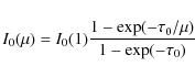
where the subscript 0 is for the line center and
and a fit of the observed
For the lines for which only the line radiance E is known (S VI 94.4 nm and Ly
![]() ), we need to fit the following function, where
), we need to fit the following function, where ![]() and E(1) are parameters
and E(1) are parameters![]() :
:
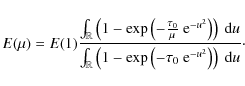
This expression is derived from Dumont et al. (1983) and assumes a Doppler absorption profile
These theoretical functions of ![]() are then plotted for different values of the parameter
are then plotted for different values of the parameter ![]() over the observations in Fig. 3, for all three lines (either for the peak
spectral radiance or the line radiance, depending on the data). We performed a non-linear least squares fit with the Levenberg-Marquardt algorithm as implemented in the Interactive Data
Language (IDL) to estimate the parameter
over the observations in Fig. 3, for all three lines (either for the peak
spectral radiance or the line radiance, depending on the data). We performed a non-linear least squares fit with the Levenberg-Marquardt algorithm as implemented in the Interactive Data
Language (IDL) to estimate the parameter ![]() .
The uncertainties in each point of the
.
The uncertainties in each point of the ![]() or
or ![]() functions (an average of
functions (an average of ![]() pixels) that we take as input to the fitting procedure come mainly from the possible presence of coherent structures such as bright points: the number of possible structures is of the order
pixels) that we take as input to the fitting procedure come mainly from the possible presence of coherent structures such as bright points: the number of possible structures is of the order
![]() ,
where
,
where ![]() is the size of these structures (we assume
is the size of these structures (we assume
![]() pixels), and then the uncertainty in I or E is
pixels), and then the uncertainty in I or E is
![]() where
where ![]() is the standard deviation of the data points
(in each pixel of a
is the standard deviation of the data points
(in each pixel of a ![]() bin). Compared to this uncertainty, the photon noise is negligible.
bin). Compared to this uncertainty, the photon noise is negligible.
The results of the fits for the interval
![]() are shown in Fig. 3: as far as
are shown in Fig. 3: as far as ![]() is concerned, they are 0.113 for moment (1) (S VI 93.3 nm peak spectral radiance) and 0.244 for moment (5) (S VI 94.4 nm radiance, blended with Si VIII). The approximations that we used in writing Eq. (1) are invalid for the optically thick Ly
is concerned, they are 0.113 for moment (1) (S VI 93.3 nm peak spectral radiance) and 0.244 for moment (5) (S VI 94.4 nm radiance, blended with Si VIII). The approximations that we used in writing Eq. (1) are invalid for the optically thick Ly
![]() line, which should explain the poor fit. On the other hand, these approximations are valid for both the S VI lines, as long as
line, which should explain the poor fit. On the other hand, these approximations are valid for both the S VI lines, as long as ![]() is small enough. For large
is small enough. For large ![]() ,
there is an additional uncertainty resulting from the determination of the limb.
,
there is an additional uncertainty resulting from the determination of the limb.
These results are sensitive to the limb fitting: a 10-3 relative error in the determination of the solar radius leads to a 7 ![]() 10-2 relative error in
10-2 relative error in ![]() .
Since 10-3 is a conservative upper limit to the error in the radius from the limb fitting, we can consider 7
.
Since 10-3 is a conservative upper limit to the error in the radius from the limb fitting, we can consider 7 ![]() 10-2 to be a conservative estimate of the relative error in
10-2 to be a conservative estimate of the relative error in ![]() resulting
from the limb fitting.
resulting
from the limb fitting.
![\begin{figure}
\par\includegraphics[width=8.5cm,clip]{11588f3}
\end{figure}](/articles/aa/full_html/2009/32/aa11588-08/img72.png) |
Figure 3:
Diamonds: average profiles of the radiance data (moments 1, 4 and 5) as a function of |
| Open with DEXTER | |
3.2 Using center-to-limb ratios of S VI 93.3 nm width and radiance
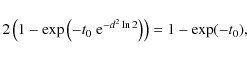
The variation with position of the S VI 93.3 nm line width (see Fig. 2) can be interpreted as an opacity saturation of the S VI 93.3 nm line at the limb, and method B of Dumont et al. (1983) can then
be applied. This method relies on the measurement of the ratio
![]() of the FWHM at the limb and the disk center: the optical thickness at line center t0 at the limb is given by solving
of the FWHM at the limb and the disk center: the optical thickness at line center t0 at the limb is given by solving
 |
(4) |
which is Eq. (4) of Dumont et al. (1983), where a sign error has been corrected, and the opacity at line center
 |
(5) |
Using the full-Sun S VI 93.3 nm compressed data set DS1
3.3 Using the S VI 94.4 - 93.3 line ratio
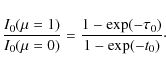
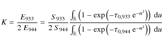
The theoretical dependence of the S VI 94.4 - 93.3 peak radiance line ratio as a function of the line opacities and source functions is
 |
(6) |
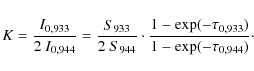
For this doublet, we assume S933 = S944 and
 |
(7) |
and we derive
| (8) |
The difficulty is that the S VI 94.4 nm line is blended with the Si VIII line. To remove this blend, we analyzed the line profiles available in data set DS2. After averaging the line profiles over the 60 central pixels along the slit, we fitted the S VI 93.3 nm line with a Gaussian and a uniform background, and the S VI 94.4 nm line blend with two Gaussians and a uniform background. We then computed the Gaussian amplitude from these fits for both S VI lines, to measure I0,933 and I0,944, and then K, which we averaged over all observations. From this method, we inferred that
The same kind of method could in theory be used for the S VI 94.4 - 93.3 line radiance ratio
with, again, S933 = S944 and
3.4 Discussion about opacity determination
It is clear that the three methods provide different values of the opacity at disk center. We confirm the result of Dumont et al. (1983), obtained in different lines, by which the method of center-to-limb ratios of width and radiance (Sect. 3.2, or method B in Dumont et al. 1983) provides the smallest value of the opacity. As mentioned by these authors, the center-to-limb variation method (Sect. 3.1, or method A) overestimates the opacity for different reasons described in Dumont et al. (1983), including the curvature of the layers close to the limb and their roughness. The method of line ratios (Sect. 3.3, or method C) also provides larger values of the opacity, although free from geometrical assumptions; Dumont et al. (1983) interpret them as resulting from a difference between the source functions of the lines of the doublet.
This does not mean that there are no additional biases. For instance, we adopted a constant Doppler width from center to limb; this is incorrect since, at the limb, the observed layer is at higher altitude, where the temperature and turbulence are higher than in the emitting layer as viewed at disk center. Consequently, the excessive line width is wrongly interpreted as only an opacity effect. However, it seems improbable that a ![]() increase in Doppler width from center
to limb can be interpreted entirely in terms of temperature (because of the square-root temperature variation in Doppler width) and turbulence (since the emitting layer is - a posteriori - optically
not very thick).
increase in Doppler width from center
to limb can be interpreted entirely in terms of temperature (because of the square-root temperature variation in Doppler width) and turbulence (since the emitting layer is - a posteriori - optically
not very thick).
4 First estimates of densities
4.1 Densities using the opacities
The line-of-sight opacity at line center of the S VI 93.3 nm line is given by
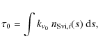
where the integration is along the line-of-sight. The variable
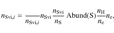
where
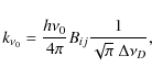
where Bij is the Einstein absorption coefficient for the transition
 |
(13) |
with gj / gi = 2 and
 |
(14) |
Finally, for an emitting layer of thickness
Taking
4.2 Squared densities using the contribution function
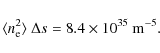
The average S VI 93.3 nm line radiance at disk center obtained from data set DS2 (excluding the 5% higher values not considered to be part of the quiet Sun) is E = 1.4 ![]()
![]() (compared to the value 3.81
(compared to the value 3.81 ![]() 10-3 given by CHIANTI with
a quiet Sun DEM - see Table 1). This can be used to estimate
10-3 given by CHIANTI with
a quiet Sun DEM - see Table 1). This can be used to estimate
![]() in the emitting region of thickness
in the emitting region of thickness ![]() ,
since
,
since
where G(T) is the contribution function, the integral is evaluated along the line-of-sight, and we assume that
gofnt function of CHIANTI infers
 |
(17) |
Again for
5 Discussion of biases in the method
At the start of this work, one of our aims was to determine a filling factor![]()

in the S VI-emitting region. This initial objective needs to be reviewed, because we obtain f=144, an impossible value as it is more than 1. Our values of densities can be compared with the density at
Given the same measurements of ![]() and E, one can instead assume of a filling factor
and E, one can instead assume of a filling factor ![]() and infer
and infer ![]() to be
to be
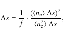
where the numerator and denominator of the second quotient in the product shown are determined from Eqs. (15) and (16) respectively. With the values from Sect. 4, this gives
In any case, there seems to be some inconsistencies for
![]() between on the one hand our new observations of opacities, and on the other hand transition region models and observations of intensities. We now propose to discuss the possible sources of these discrepancies, while releasing, when needed, some of the simplistic assumptions we have so far made.
between on the one hand our new observations of opacities, and on the other hand transition region models and observations of intensities. We now propose to discuss the possible sources of these discrepancies, while releasing, when needed, some of the simplistic assumptions we have so far made.
5.1 Assumption of a uniform emitting layer
5.1.1 Bias due to this assumption
When computing the average densities from the S VI 93.3 nm opacity and radiance, we assumed a uniform emitting layer at the temperature of maximum emission and of thickness ![]() given by the width of contribution function G(T). However, the different dependences of the electron density in Eqs. (10) and (16) - the first is linear while the second is quadratic - means that the slope of the
given by the width of contribution function G(T). However, the different dependences of the electron density in Eqs. (10) and (16) - the first is linear while the second is quadratic - means that the slope of the
![]() function affects the weights on the integrals of Eqs. (10) and (16) differently: a bias, different for
function affects the weights on the integrals of Eqs. (10) and (16) differently: a bias, different for ![]() and E, can be expected, and here we explore this effect starting from the Avrett & Loeser (2008) model, which has the merit of giving average profiles of temperature and density (among other variables) as a function of altitude s.
and E, can be expected, and here we explore this effect starting from the Avrett & Loeser (2008) model, which has the merit of giving average profiles of temperature and density (among other variables) as a function of altitude s.
Opacity.
Using the Avrett & Loeser (2008) profiles and atomic physics data, we derive
Radiance.
Using the same Avrett & Loeser (2008) profiles and the CHIANTI contribution function G(T), we derive E = 1.3
We see then that the assumption of a uniform emitting layer has a bias towards high densities, which is stronger for the opacity method than for the radiance method. A filling factor computed from these values would be f=1.5, while it was assumed to be 1 when computing ![]() and E from the Avrett & Loeser (2008) model: this can be one of the reasons for our too high observed filling factor.
and E from the Avrett & Loeser (2008) model: this can be one of the reasons for our too high observed filling factor.
This differential bias acts surprisingly because, according to the
![]() term in Eq. (16) one would expect the bias to be stronger for E than for
term in Eq. (16) one would expect the bias to be stronger for E than for ![]() ;
however, it can be understood by
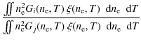
comparing the effective temperatures for
;
however, it can be understood by
comparing the effective temperatures for ![]() and E, which are respectively
and E, which are respectively
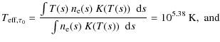
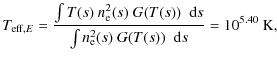
where
It can be pointed out that the difference between the K(T) and G(T) kernels is present because G(T) (unlike K(T)) takes into account not only the ionization equilibrium of S VI, but also the collisions from i to j levels of S VI ions.
5.1.2 Releasing this assumption: a tentative estimate of the density gradient around log T = 5.3
In Sect. 5.1.1 we have demonstrated that the radiance computed with the Avrett & Loeser (2008) profiles and the CHIANTI contribution function G(T) is a factor of 3 higher than the radiance computed directly by CHIANTI using the standard quiet Sun DEM (see Table 1). This is because the DEM computed from the temperature and density profiles of the Avrett & Loeser (2008) model differs from the CHIANTI DEM![]() , as can be seen in Fig. 4. In particular, the Avrett & Loeser (2008) DEM is missing the dip around
, as can be seen in Fig. 4. In particular, the Avrett & Loeser (2008) DEM is missing the dip around
![]() inferred from most observations; at
inferred from most observations; at
![]() ,
it is a factor of 3 higher than the CHIANTI quiet Sun DEM.
,
it is a factor of 3 higher than the CHIANTI quiet Sun DEM.
![\begin{figure}
\par\includegraphics[width=8.5cm,clip]{11588f4}
\end{figure}](/articles/aa/full_html/2009/32/aa11588-08/img135.png) |
Figure 4:
Quiet Sun standard DEM from CHIANTI (plain line) and DEM
computed from the Avrett & Loeser (2008) temperature and density
profiles dashed lines. The dotted lines represent the DEMs for
|
| Open with DEXTER | |
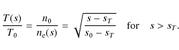
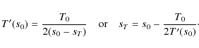
We model the upper transition region locally around
![]() and
and
![]() (chosen because
T(s0) = T0 in the Avrett & Loeser 2008 model) by a vertically stratified plasma at
pressure
P0 = 1.91 n0 kB T0 (we consider a fully ionized coronal plasma) and
(chosen because
T(s0) = T0 in the Avrett & Loeser 2008 model) by a vertically stratified plasma at
pressure
P0 = 1.91 n0 kB T0 (we consider a fully ionized coronal plasma) and
 |
(22) |
These equations were chosen to provide a good approximation to a transition region, with some symmetry between the opposite curvatures of the variations in T and
 |
(23) |
In Fig. 5, we plot some temperature profiles from this simple transition region model, for different model parameters T'(s0) (P0 only affects the scale of
![\begin{figure}
\par\includegraphics[width=8.5cm,clip]{11588f5}
\end{figure}](/articles/aa/full_html/2009/32/aa11588-08/img142.png) |
Figure 5:
Temperature as a function of altitude in our local transition region simple models around
T0 = 105.3 and
|
| Open with DEXTER | |
We propose to use these models along with atomic physics data and the equations in Sect. 4 to compute ![]() and E as a function of the model parameters P0 and T'(s0), as shown in Fig. 6. Since the slopes of the level lines
differs in the
and E as a function of the model parameters P0 and T'(s0), as shown in Fig. 6. Since the slopes of the level lines
differs in the
![]() and
E(P0,T'(s0)) plots, one would in theory be able to estimate the parameters
(P0, T'(s0)) of the best fit model for the observation of
and
E(P0,T'(s0)) plots, one would in theory be able to estimate the parameters
(P0, T'(s0)) of the best fit model for the observation of
![]() by simply finding the crossing between the level lines
by simply finding the crossing between the level lines
![]() and
and
![]() .
.
In practice however, the level lines for our observations of ![]() and E do not intersect in the range of parameters plotted in Fig. 6, corresponding to realistic values of the
parameters. As a consequence, it is impossible to infer from these measurements (from a single spectral line, here S VI 93.3 nm) the temperature slope and the density of the TR around the formation of this line.
and E do not intersect in the range of parameters plotted in Fig. 6, corresponding to realistic values of the
parameters. As a consequence, it is impossible to infer from these measurements (from a single spectral line, here S VI 93.3 nm) the temperature slope and the density of the TR around the formation of this line.
If we now extend the range of T'(s0) to unrealistically low values, a crossing of the level lines can be found below
![]() and
and
![]() .
Given the width of G(T) for S VI 93.3 nm, this corresponds to
.
Given the width of G(T) for S VI 93.3 nm, this corresponds to
![]() ,
a value consistent with that obtained from Eq. (19), which is also much larger than expected.
,
a value consistent with that obtained from Eq. (19), which is also much larger than expected.
We note that Keenan (1988) derived a much lower S VI 93.3 nm opacity value (
![]()
![]() 10-4 at disk center) from a computation implying the cells of the network model of Gabriel (1976). However, while our value of
10-4 at disk center) from a computation implying the cells of the network model of Gabriel (1976). However, while our value of ![]() seems to be too high, the level lines in Fig. 6 show that an opacity value
seems to be too high, the level lines in Fig. 6 show that an opacity value
![]()
![]() 10-4 would be too low: from this figure we expect that a value compatible with radiance measurements and realistic values of the temperature gradient would be in the range 5
10-4 would be too low: from this figure we expect that a value compatible with radiance measurements and realistic values of the temperature gradient would be in the range 5 ![]() 10-3 to 10-2.
10-3 to 10-2.
![\begin{figure}
\par\includegraphics[width=8.5cm,clip]{11588f6a}\vspace*{1.5mm}
\...
...588f6b}\vspace*{1.5mm}
\includegraphics[width=8.5cm,clip]{11588f6c}
\end{figure}](/articles/aa/full_html/2009/32/aa11588-08/img151.png) |
Figure 6:
S VI 93.3 nm opacity |
| Open with DEXTER | |
5.2 Anomalous behavior of Na-like ions
Following work by Dupree (1972) for Li-like ions, Judge et al. (1995) report that standard DEM analysis fails for ions of the Li and Na isoelectronic sequences; in particular, for S VI (which is Na-like), Del Zanna et al. (2001) find that the atomic physics models underestimate the S VI 93.3 nm line radiance E by a factor of 3. This fully explains the difference between our observation of E and the value computed by CHIANTI (Table 1). However, this also means that where G(T) from CHIANTI is used, as in Eq. (16), it presumably needs to be multiplied by 3. As a result, one can expect
![]() to be lower by a factor 1.7, resulting in a filling factor
of 415, which is poorer than our initial result.
to be lower by a factor 1.7, resulting in a filling factor
of 415, which is poorer than our initial result.
The reasons for the anomalous behavior of these ions for G(T), which could be linked to either ionization equilibrium or collisions, are still unknown. As a result, it is impossible to tell whether these reasons also produce an anomalous behavior of these ions for K(T), hence in our measurements of opacities and estimates of densities: this could again reduce the filling factor.
5.3 Cell-and-network pattern
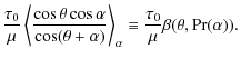
When analyzing our observations, we have not made the distinction between the network lanes and the cells of the chromospheric supergranulation. Here we try to evaluate the effect of the supergranular pattern on our measurements by using a 2D model emitting layer with a simple ``paddle wheel'' cell-and-network pattern: in polar coordinates
![]() ,
the emitting layer is defined by R1<r<R2; in the emitting layer, the network lanes are defined by
,
the emitting layer is defined by R1<r<R2; in the emitting layer, the network lanes are defined by
![]() and the cells are in the other parts of the emitting layer, where
and the cells are in the other parts of the emitting layer, where
![]() is the pattern angular cell size (an integer fraction of
is the pattern angular cell size (an integer fraction of ![]() )
and
)
and
![]() is the network lane angular size. The network lanes and cells are characterized by different (but uniform) source functions S, densities
is the network lane angular size. The network lanes and cells are characterized by different (but uniform) source functions S, densities
![]() ,
and absorption coefficients
,
and absorption coefficients ![]() .
We then solve the radiative transfer equations for
.
We then solve the radiative transfer equations for ![]() along rays
originating in infinity through the emitting layer to the observer.
along rays
originating in infinity through the emitting layer to the observer.
Since the opacity is obtained by a simple integration of
![]() ,
the average line-of-sight opacity t0 as a function of
,
the average line-of-sight opacity t0 as a function of ![]() for the ``paddle-wheel'' pattern is the same as for a uniform layer with the same average
for the ``paddle-wheel'' pattern is the same as for a uniform layer with the same average
![]() .
However, as seen in Fig. 7, still for the same average S and
.
However, as seen in Fig. 7, still for the same average S and
![]() ,
the effect of opacity (a decrease in intensity) is higher in the ``paddle-wheel'' case, in particular for intermediate values of
,
the effect of opacity (a decrease in intensity) is higher in the ``paddle-wheel'' case, in particular for intermediate values of ![]() .
As a result, neglecting the cell-and-network pattern of the true TR leads to overestimation of the opacity when using method A.
.
As a result, neglecting the cell-and-network pattern of the true TR leads to overestimation of the opacity when using method A.
![\begin{figure}
\par\includegraphics[width=8.5cm,clip]{11588f7}
\end{figure}](/articles/aa/full_html/2009/32/aa11588-08/img160.png) |
Figure 7:
Average spectral radiance at line center I0 as a function of |
| Open with DEXTER | |
5.4 Roughness and fine structure
To explain the high values of opacity (as derived from their method A), Dumont et al. (1983) introduce the concept of roughness of the TR: since the TR plasma is not perfectly vertically stratified (there is some horizontal variation), method A leads to an overestimated value of ![]() .
This could reconcile the values obtained following our application of methods A and B.
.
This could reconcile the values obtained following our application of methods A and B.
We model the roughness of the transition region by incompressible vertical displacements of any given layer (at given optical depth) from its average vertical position, in the geometry shown in
Fig. 8. The layer then forms an angle ![]() with the horizontal and has still the same vertical thickness
with the horizontal and has still the same vertical thickness
![]() ;
the thickness along the LOS is
;
the thickness along the LOS is
![]() ,
as can be deduced from Fig. 8.
,
as can be deduced from Fig. 8.
If we assume that
![]() remains sufficiently small for the plane-parallel approximation to hold (and so that the LOS crosses one given layer only once), the opacity is
remains sufficiently small for the plane-parallel approximation to hold (and so that the LOS crosses one given layer only once), the opacity is
| (24) |
The angle
| |
= | (25) | |
| = |  |
(26) |
The opacity
We immediately see that ![]() for
for
![]() ,
for any
,
for any
![]() :
roughness (as modeled here by incompressible vertical displacements) does not change the optical thickness at disk center.
Nevertheless, the estimate of optical thickness at disk center from observations in Sect. 3.1 (method A of Dumont et al. 1983) is affected by this roughness effect.
:
roughness (as modeled here by incompressible vertical displacements) does not change the optical thickness at disk center.
Nevertheless, the estimate of optical thickness at disk center from observations in Sect. 3.1 (method A of Dumont et al. 1983) is affected by this roughness effect.
| |
Figure 8:
Geometry of a TR layer (plain contour), displaced from its average position (dashed contour) while retaining its original vertical thickness
|
| Open with DEXTER | |
![\begin{figure}
\par\includegraphics[width=8.5cm,clip]{11588f9}
\end{figure}](/articles/aa/full_html/2009/32/aa11588-08/img175.png) |
Figure 9: Multiplicative coefficient to t0 due to roughness, for different roughness parameters A. |
| Open with DEXTER | |
Coming back to
![]() ,
we take
,
we take
![]() ,
and we compute
,
and we compute ![]() numerically (A represents the width of
numerically (A represents the width of
![]() and can be considered to be a
quantitative measurement of the roughness). The results, shown in Fig. 9, indicate for example that the modeled roughness with
and can be considered to be a
quantitative measurement of the roughness). The results, shown in Fig. 9, indicate for example that the modeled roughness with ![]() increases the opacity by
increases the opacity by ![]() at
at ![]() (corresponding to
(corresponding to
![]() ). This is a significant effect, and we can evaluate its influence on the estimate of
). This is a significant effect, and we can evaluate its influence on the estimate of ![]() in Sect. 3.1: in the theoretical profiles of
in Sect. 3.1: in the theoretical profiles of ![]() and
and ![]() (Eqs. (2), (3)),
(Eqs. (2), (3)),
![]() needs to be replaced by
needs to be replaced by
![]() .
Since
.
Since ![]() for a rough corona, this means that the value of
for a rough corona, this means that the value of ![]() determined from the fit of observed radiances to Eqs. (2), (3) is overestimated by a factor corresponding approximately to the mean value of
determined from the fit of observed radiances to Eqs. (2), (3) is overestimated by a factor corresponding approximately to the mean value of ![]() for the fitting range.
for the fitting range.
In this way, we have estimated quantitatively the overestimation factor of ![]() by the method of Sect. 3.1, thus extending the qualitative discussion of roughness found in
Dumont et al. (1983). This factor, of the order of 1.1 may seem modest, but one needs to remember that the fit for obtaining
by the method of Sect. 3.1, thus extending the qualitative discussion of roughness found in
Dumont et al. (1983). This factor, of the order of 1.1 may seem modest, but one needs to remember that the fit for obtaining ![]() in Sect. 3.1 was completed for a wide range (
in Sect. 3.1 was completed for a wide range (![]() from 1 to 5, or
from 1 to 5, or ![]() from 0 to 78 degrees) that our roughness model cannot reproduce entirely
from 0 to 78 degrees) that our roughness model cannot reproduce entirely![]() .
.
One can consider different roughness models that represent the strong inhomogeneity of the TR. For instance with a different and very peculiar roughness model, Pecker et al. (1988) obtained an overestimation factor of more than 10 under some conditions. This means that our values of ![]() may need to be decreased by a large factor because of a roughness effect.
may need to be decreased by a large factor because of a roughness effect.
Roughness models can be seen as simplified models of the fine structure of the TR, which is known to be heterogeneous on small scales. Indeed, in addition to the chromospheric network pattern that we modeled in Sect. 5.3, the TR contains parts of different structures, with different plasma properties, such as the base of large loops and coronal funnels, smaller loops (Peter 2001; Dowdy et al. 1986), and spicules. Furthermore, the loops themselves are likely to consist of strands, which can be heated independently (Parenti et al. 2006; Cargill & Klimchuk 2004). The magnetic field in these structures inhibits perpendicular transport, and as a consequence the horizontal inhomogeneities are not smoothed out efficiently.
6 Conclusion
We have derived the average electron density in the TR from the opacity ![]() of the S VI 93.3 nm line, which was obtained by three different methods from observations of the full Sun: center-to-limb variation in radiance, center-to-limb ratios of radiance and line width, and radiance ratio of the
of the S VI 93.3 nm line, which was obtained by three different methods from observations of the full Sun: center-to-limb variation in radiance, center-to-limb ratios of radiance and line width, and radiance ratio of the
![]() doublet. Assuming a spherically symmetric plane-parallel layer of constant source function, we found a S VI 93.3 nm opacity of the order of 0.05. The derived average electron density is of the order of 2.4
doublet. Assuming a spherically symmetric plane-parallel layer of constant source function, we found a S VI 93.3 nm opacity of the order of 0.05. The derived average electron density is of the order of 2.4 ![]()
![]() .
.
We have then used the line radiance (by an EM method) to derive the rms average electron density in the S VI 93.3 nm-emitting region and obtained 2.0 ![]()
![]() .
This corresponds to a total pressure of
.
This corresponds to a total pressure of
![]() ,
slightly higher than the range of pressures found by Dumont et al. (1983) (1.3 to 6.3
,
slightly higher than the range of pressures found by Dumont et al. (1983) (1.3 to 6.3 ![]()
![]() ,
as deduced from their Sect. 4.2), but lower than the value given in Mariska (1993) (2
,
as deduced from their Sect. 4.2), but lower than the value given in Mariska (1993) (2 ![]()
![]() ).
).
The average electron densities obtained from these methods (opacity on the one hand, radiance on the other hand) are incompatible, as can be seen either from a direct comparison of the values of
![]() and
and
![]() for a given thickness
for a given thickness ![]() of a uniform emitting layer, or by computing the
of a uniform emitting layer, or by computing the ![]() that would reconcile the measurements of
that would reconcile the measurements of
![]() and
and
![]() .
Furthermore, we have seen that the density obtained from the opacity method is also
incompatible with standard DEMs of the Quiet Sun (see Sect. 4.2) and with semi-empirical models of the temperature and density profiles in the TR (see Sect. 5.1.2).
.
Furthermore, we have seen that the density obtained from the opacity method is also
incompatible with standard DEMs of the Quiet Sun (see Sect. 4.2) and with semi-empirical models of the temperature and density profiles in the TR (see Sect. 5.1.2).
We investigated several possible sources of biases in the determination of ![]() :
the approximation of a constant temperature in the S VI emitting layer, the anomalous behavior of the S VI ion, the chromospheric network pattern, and the roughness of the TR. Some of these could help explain partly the discrepancy between the average densities deduced from opacities and from radiances, but there is still a long way to go to fully understand this discrepancy and to reconcile the measurements. At this stage, we can only encourage colleagues to look for similar discrepancies in lines formed around
:
the approximation of a constant temperature in the S VI emitting layer, the anomalous behavior of the S VI ion, the chromospheric network pattern, and the roughness of the TR. Some of these could help explain partly the discrepancy between the average densities deduced from opacities and from radiances, but there is still a long way to go to fully understand this discrepancy and to reconcile the measurements. At this stage, we can only encourage colleagues to look for similar discrepancies in lines formed around
![]() (like C IV and O VI), Na-like and not
Na-like, and to repeat similar S VI center-to-limb measurements.
(like C IV and O VI), Na-like and not
Na-like, and to repeat similar S VI center-to-limb measurements.
In Sect. 5.1.2, we tried to combine opacity and radiance information to compute the gradient of temperature. This appeared to be impossible (if restricting ourselves to a realistic
range of parameters) because of the above-mentioned incompatibility. We have estimated that a value ![]() of the S VI 93.3 nm opacity compatible with radiance measurements and with realistic values of the temperature gradient should be in the range 5
of the S VI 93.3 nm opacity compatible with radiance measurements and with realistic values of the temperature gradient should be in the range 5 ![]() 10-3 to 10-2.
10-3 to 10-2.
In spite of the difficulties that we met, we still think that the combination of opacity and radiance information should be a powerful tool for investigating the thermodynamic properties and the fine structure of the TR. For instance, the excess opacity derived from observations and a plane-parallel model could be used to evaluate models of roughness and the fine structure of the TR. Clearly, progress in modelling the radiative output of the complex structure of the TR needs to be made to achieve this.
Acknowledgements
The authors thank G. del Zanna, E. H. Avrett and Ph. Lemaire for interesting discussions and the anonymous referee for suggestions concerning this paper. The SUMER project is supported by DLR, CNES, NASA and the ESA PRODEX Programme (Swiss contribution). SoHO is a project of international cooperation between ESA and NASA. Data was provided by the MEDOC data center at IAS, Orsay. E.B. thanks CNES for financial support, and the ISSI group on Coronal Heating (S. Parenti). CHIANTI is a collaborative project involving the NRL (USA), RAL (UK), MSSL (UK), the Universities of Florence (Italy) and Cambridge (UK), and George Mason University (USA).
Appendix A: About the filling factor
In this paper, we have defined the filling factor as
 |
(A.1) |
while it is usually inferred from solar observations (e.g. Judge 2000; Klimchuk & Cargill 2001) to be

where EM is the emission measure,
It may seem surprising that the EM is in the numerator of this second expression, while it provides an estimate for
![]() ,
which appears in the denominator of the first expression. However, we can show that both expressions, despite looking very different, actually
provide the same result for a given plasma.
,
which appears in the denominator of the first expression. However, we can show that both expressions, despite looking very different, actually
provide the same result for a given plasma.
We assume a plasma with a differential distribution
![]() for the density and temperature, i.e.,
for the density and temperature, i.e.,
![]() is the proportion of any given volume occupied by plasma at a density between
is the proportion of any given volume occupied by plasma at a density between
![]() and
and
![]() ,
and a temperature between T and
,
and a temperature between T and
![]() .
.
The contributions to both the line radiance E and the opacity at line center ![]() from a volume V with this plasma distribution are
from a volume V with this plasma distribution are
| (A.3) | |||
| (A.4) |
with the usual notations of our article.
The usual assumption (e.g. Judge 2000) is that
![]() ``selects'' a narrow range of temperatures around
``selects'' a narrow range of temperatures around
![]() and does not depend on
and does not depend on
![]() ,
i.e.,
,
i.e.,
![]() .
Similarly, we can consider that
.
Similarly, we can consider that
![]() . Then
. Then
| (A.5) | |||
| (A.6) |
Following Judge (2000) and for the assumption
| |
= |  |
(A.7) |
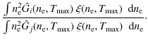 |
(A.8) |
When homogeneity is assumed, i.e.,
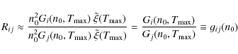 |
(A.9) |
and inverting this function allows us to recover n0 from the observed value of Rij.
The fundamental point is that Rij does not depend on the proportion f (the filling factor) of the volume occupied by the plasma, and n0 is the density in the non-void region only. For
example, for
![]() defined by
defined by
![]() ,
the line ratio Rij is
gij(n0), which is independent of f, while
,
the line ratio Rij is
gij(n0), which is independent of f, while
![]() determined from E/V would be f n02, and
determined from E/V would be f n02, and
![]() determined from
determined from ![]() would be f n0. In this case, one can see that f can (equivalently) either be recovered from
would be f n0. In this case, one can see that f can (equivalently) either be recovered from
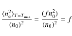 |
(A.10) |
(corresponding to Judge 2000) or from
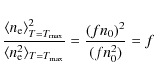 |
(A.11) |
(corresponding to our method).
References
- Avrett, E. H., & Loeser, R. 2008, ApJS, 175, 229 [NASA ADS] [CrossRef]
- Buchlin, E., Vial, J.-C., & Lemaire, P. 2006, A&A, 451, 1091 [NASA ADS] [CrossRef] [EDP Sciences] (In the text)
- Cargill, P. J., & Klimchuk, J. A. 2004, ApJ, 605, 911 [NASA ADS] [CrossRef]
- Curdt, W., Brekke, P., Feldman, U., et al. 2001, A&A, 375, 591 [NASA ADS] [CrossRef] [EDP Sciences]
- Del Zanna, G., Bromage, B. J. I., & Mason, H. E. 2001, in Joint SOHO/ACE workshop, Solar and Galactic Composition, ed. R. F. Wimmer-Schweingruber, AIP Conf. Ser., 598, 59 (In the text)
- Dere, K. P., Landi, E., Mason, H. E., Monsignori Fossi, B. C., & Young, P. 1997, A&AS, 125, 149 [NASA ADS] [CrossRef] [EDP Sciences]
- Dowdy, J. F., Rabin, D., & Moore, R. L. 1986, Sol. Phys., 105, 35 [NASA ADS] [CrossRef]
- Dumont, S., Pecker, J.-C., Mouradian, Z., Vial, J.-C., & Chipman, E. 1983, Sol. Phys., 83, 27 [NASA ADS] [CrossRef] (In the text)
- Dupree, A. K. 1972, ApJ, 178, 527 [NASA ADS] [CrossRef] (In the text)
- Gabriel, A. 1976, R. Soc. London Phil. Trans. Ser. A, 281, 339 [NASA ADS] [CrossRef] (In the text)
- Judge, P. G. 2000, ApJ, 531, 585 [NASA ADS] [CrossRef]
- Judge, P. G., Woods, T. N., Brekke, P., & Rottman, G. J. 1995, ApJ, 455, L85 [NASA ADS] [CrossRef] (In the text)
- Keenan, F. P. 1988, Sol. Phys., 116, 279 [NASA ADS] (In the text)
- Klimchuk, J. A., & Cargill, P. J. 2001, ApJ, 553, 440 [NASA ADS] [CrossRef]
- Landi, E., Del Zanna, G., Young, P. R., et al. 2006, ApJS, 162, 261 [NASA ADS] [CrossRef]
- Mariska, J. T. 1993, The Solar Transition Region (Cambridge University Press)
- Mason, H. E. 1998, in Space Solar Physics: Theoretical and Observational Issues in the Context of the SOHO Mission, ed. J. C. Vial, K. Bocchialini, & P. Boumier, Lecture Notes in Physics (Berlin: Springer Verlag), 507, 143 (In the text)
- Parenti, S., Buchlin, E., Cargill, P. J., Galtier, S., & Vial, J.-C. 2006, ApJ, 651, 1219 [NASA ADS] [CrossRef]
- Pecker, J.-C., Dumont, S., & Mouradian, Z. 1988, A&A, 196, 269 [NASA ADS] (In the text)
- Peter, H. 1999, ApJ, 516, 490 [NASA ADS] [CrossRef]
- Peter, H. 2001, A&A, 374, 1108 [NASA ADS] [CrossRef] [EDP Sciences]
- Peter, H., & Judge, P. G. 1999, ApJ, 522, 1148 [NASA ADS] [CrossRef]
- Wilhelm, K., Curdt, W., Marsch, E., et al. 1995, Sol. Phys., 162, 189 [NASA ADS] [CrossRef]
Footnotes
- ... formed
![[*]](/icons/foot_motif.png)
- We release this assumption in Sect. 5.
- ... parameters
- Note that, in contrast to Dumont et al. (1983), we consider I0(1) as an additional parameter. This is because by doing so, we avoid the sensitivity of I0(1) to structures close to disk center, and because the first data bin starts at
 instead of being centered on .
- ... parameters
- We take here E(1) as a parameter for the same reason as we did before for I0(1).
- ... DS1
- Although not obvious from the data headers, moment (3) corresponds to the deconvoluted FWHM of S VI 93.3 nm, as confirmed by comparing with the width obtained from the full profiles in data set DS2 and deconvoluted using the Solar Software procedure con_width_4.
- ... factor
- We explain this definition of the filling factor in Appendix A.
- ... DEM
- The reason for this is that the Avrett & Loeser (2008) model is determined from theoretical energy balance and needs further improvement to reproduce the observed DEM (Avrett, private communication).
- ...entirely
- For high values of the
 width A, the correction factor
  cannot be computed for high values of
(high angles
cannot be computed for high values of
(high angles  )
because the values of
)
because the values of  in the wings of
fall in the range where
in the wings of
fall in the range where
 :
the plane-parallel approximation is no longer valid. This explains the limited range of the
:
the plane-parallel approximation is no longer valid. This explains the limited range of the
 curves in Fig. 9.
All Tables
Table 1: Spectral lines present in the data sets, with parameters computed by CHIANTI and given by previous observations.
All Figures
| |
Figure 1:
Raw line profiles from the context spectrum taken on 4 May 1996 at 07:32 UT at disk center with an exposure time of
|
| Open with DEXTER | |
| In the text | |
| |
Figure 2:
Average of the data as a function of
|
| Open with DEXTER | |
| In the text | |
| |
Figure 3:
Diamonds: average profiles of the radiance data (moments 1, 4 and 5) as a function of |
| Open with DEXTER | |
| In the text | |
| |
Figure 4:
Quiet Sun standard DEM from CHIANTI (plain line) and DEM
computed from the Avrett & Loeser (2008) temperature and density
profiles dashed lines. The dotted lines represent the DEMs for
|
| Open with DEXTER | |
| In the text | |
| |
Figure 5:
Temperature as a function of altitude in our local transition region simple models around
T0 = 105.3 and
|
| Open with DEXTER | |
| In the text | |
| |
Figure 6:
S VI 93.3 nm opacity |
| Open with DEXTER | |
| In the text | |
| |
Figure 7:
Average spectral radiance at line center I0 as a function of |
| Open with DEXTER | |
| In the text | |
| |
Figure 8:
Geometry of a TR layer (plain contour), displaced from its average position (dashed contour) while retaining its original vertical thickness
|
| Open with DEXTER | |
| In the text | |
| |
Figure 9: Multiplicative coefficient to t0 due to roughness, for different roughness parameters A. |
| Open with DEXTER | |
| In the text | |
Copyright ESO 2009
Current usage metrics show cumulative count of Article Views (full-text article views including HTML views, PDF and ePub downloads, according to the available data) and Abstracts Views on Vision4Press platform.
Data correspond to usage on the plateform after 2015. The current usage metrics is available 48-96 hours after online publication and is updated daily on week days.
Initial download of the metrics may take a while.