Synchrotron self-Compton flaring of TeV blazars

C. Röken; R. Schlickeiser

doi:10.1051/0004-6361/200811250

Home

All issues

Volume 503 / No 2 (August IV 2009)

A&A, 503 2 (2009) 309-322

Full HTML

Free Access

Issue		A&A Volume 503, Number 2, August IV 2009


Page(s)		309 - 322
Section		Astrophysical processes
DOI		https://doi.org/10.1051/0004-6361/200811250
Published online		15 June 2009

II. Linear and nonlinear electron cooling

C. Röken - R. Schlickeiser

Institut für Theoretische Physik, Lehrstuhl IV: Weltraum- und Astrophysik, Ruhr-Universität Bochum, 44780 Bochum, Germany

Received 29 October 2008 / Accepted 9 May 2009

Abstract
A theoretical radiation model for the flaring of TeV blazars is discussed here for the case of a nonlinear electron synchrotron cooling in these sources. We compute analytically the optically thick and thin synchrotron radiation intensities and photon density distributions in the emission knot as functions of frequency and time followed by the synchrotron self-Compton intensity and fluence in the optically thin frequency range using the Thomson approximation of the inverse Compton cross section. At all times and frequencies, the optically thin part of the synchrotron radiation process is shown to provide the dominant contribution to the synchrotron self-Compton quantities, while the optically thick part is always negligible. Afterwards, we compare the linear to the nonlinear synchrotron radiation cooling model using the data record of PKS 2155-304 on MJD 53944 favouring a linear cooling of the injected monoenergetic electrons. The good agreement of both the linear and the nonlinear cooling model with the data supports the relativistic pickup process operating in this source.
Additionally, we discuss the synchrotron self-Compton scattering, applying the full Klein-Nishina cross section to achieve the most accurate results for the synchrotron self-Compton intensity and fluence distributions.

Key words: radiation mechanisms: non-thermal - methods: analytical - galaxies: active

1 Introduction

A process describing the energy loss of ultra-relativistic electrons in cosmic-ray sources named inverse Compton scattering has been considered to be very likely responsible for the production of the high-energy radiation emitted by active galactic nuclei. In this process, low-energy photons are scattered to higher energies by relativistic electrons within the jets of these sources. There are several possible external and internal generators of the low-energy photon field, such as the accretion disc of the central black hole (Dermer et al. 1992; Dermer & Schlickeiser 1993), the broad-line region (Sikora et al. 1994), dust surrounding the active galactic nucleus (Blazejowski et al. 2000; Arbeiter et al. 2002) or synchrotron radiation produced in the jet itself. In this work, the process of interest is the inverse Compton scattering of internal synchrotron radiation called synchrotron self-Compton scattering (Maraschi et al. 1992).

Numerical models were applied in most of the studies of this process, e.g. Mastichiadis & Kirk (1997), Dermer et al. (1997), Chiaberge & Ghisellini (1999), Sokolov et al. (2004) and Böttcher (2007). Here, we investigate analytically the influence of a nonlinear electron synchrotron cooling on the synchrotron self-Compton process following the analysis of the flaring of TeV blazars due to the synchrotron self-Compton process for a linear synchrotron radiation cooling behaviour of the injected electrons (Schlickeiser & Röken 2008), where a $\delta$ -distribution approximation (Reynolds 1982; Dermer & Schlickeiser 1993) was used for the computation of the inverse Compton scattering rate $\dot n_{\rm s}$ . Most of the calculations of photon spectra modelling quantities have been based on such rather simple approximations. Therefore, we also determine the inverse Compton scattering rate, the synchrotron self-Compton intensities and fluences for the linear and nonlinear synchrotron photon densities and electron populations for the full Klein-Nishina cross section to obtain more general results (Appendix B).

We assume that a flare of the emission knot occurs at the time t = t₀ due to a uniform instantaneous injection of monoenergetic ultra-relativistic electrons. The emission knot itself moves with a relativistic bulk speed V with respect to an external observer. We model the emission knot as a spherical magnetised, fully ionised plasma cloud of radius R consisting of cold electrons and protons with a uniform density distribution and a randomly oriented large-scale time-dependent magnetic field B(t) that adjusts itself to the actual kinetic energy density of the radiating electrons in these sources, yielding the different nonlinear synchrotron radiation cooling behaviour. This magnetic field is most likely generated from the interaction of the relativistically moving knot with the surrounding ambient intergalactic and interstellar medium that is also responsible for the injection of the ultra-relativistic particles by the relativistic pickup process (Pohl & Schlickeiser 2000; Gerbig & Schlickeiser 2007; Stockem et al. 2007). The existence of a magnetic field is mandatory for the generation of synchrotron radiation and hence, the synchrotron self-Compton process.

In our analysis we assume that the synchrotron radiation losses of relativistic electrons in a constant (linear case) or partition (nonlinear) magnetic field dominate over synchrotron self-Compton losses which also imply nonlinear electron energy losses (Schlickeiser 2009) because the energy density of the target synchrotron photons is given by an energy integral over the radiating electron distribution function. Therefore, our analysis applies to blazar sources where the observed low-energy synchrotron component in the spectral energy distribution dominates over the high-energy synchrotron self-Compton component. Apart from the exceptional $\gamma$ -ray flare in July 2006 (Aharonian et al. 2009a) this applies in particular to the powerful blazar PKS 2155-304 as the existing multifrequency campaigns of this source indicate (see Fig. 10 of Aharonian et al. 2005; Fig. 2 of Aharonian et al. 2009b), especially in low activity states. We therefore compare our results with the high-energy observations from this source.

Before starting the analysis we explain our assumption that magnetic field partition is instantaneously established as the electrons cool. Equipartition conditions are often invoked in astrophysical sources for convenience, as discussed e.g. in the review by Beck & Krause (2005). Observationally, for a variety of non-thermal sources the equipartition concept is supported by magnetic field estimates such as e.g. the Coma cluster of galaxies (Schlickeiser et al. 1987). From a theoretical point of view, there is no simple explanation of partition but we will outline the basic arguments here. An upper limit on the magnetic field strength can be derived by applying Chandrasekhar's (1961, p. 583) general result, derived from the virial theorem, that for the existence of a stable equilibrium in the radiating source it is necessary that the total magnetic field energy of the system does not exceed the system's gravitational potential energy. Such a magnetic field upper limit corresponds to lower limits on the system's parallel and perpendicular plasma betas, $\beta _{\parallel }=8\pi nk_BT_\parallel / B^2$ and $\beta _{\perp }=8\pi nk_BT_\perp / B^2$ , respectively, as bi-Maxwellian plasma distributions with different temperatures along and perpendicular to the magnetic field are the most likely distributions of cosmic plasmas. The solar wind plasma is the only cosmic plasma where detailed in-situ satellite observations of plasma properties are available (Bale 2008). Ten years of Wind/SWE data (Kasper et al. 2002) have demonstrated that the proton and electron temperature anisotropies $T_\perp/T_\parallel$ are bounded by ion cyclotron, mirror and firehose instabilities (Hellinger et al. 2002) at large values of the parallel plasma beta $\beta _\parallel$ . In the parameter plane defined by the temperature anisotropy $T_\perp/T_\parallel$ and the parallel plasma beta $\beta _\parallel$ , stable plasma configurations are only possible within a rhomb-like configuration around $\beta _\parallel \simeq 1$ , whose limits are defined by the threshold conditions for these instabilities. If a plasma would start with parameter values outside this rhomb-like configuration, it immediately would generate fluctuations via the instabilities, which quickly relax the plasma distribution into the stable regime within the rhomb-configuration. Similar anisotropic plasma distributions, such as relativistic kappa-distributions, are to be expected during the pickup of interstellar particles by the interaction of the relativistic jet in the case of blazars with the surrounding ambient interstellar or intergalactic medium (Stockem et al. 2007). Such an interaction is a prominent example of the relativistic collision of plasma shells with different properties (temperature, density, composition etc.). Experimentally (Kapetanakos 1974; Tatarakis et al. 2003) and from numerous particle-in-cell (PIC) simulations (e.g. Lee & Lampe 1973; Nishikawa et al. 2003; Silva et al. 2003; Frederiksen et al. 2004; Sakai et al. 2004; Jaroschek et al. 2005) such collisions of plasma shells lead to the onset of linear Weibel-type plasma instabilities perpendicular to the flow directions in both unmagnetised and slightly magnetised plasmas, and to the development of anisotropic relativistic plasma distributions. The PIC simulations of electron-proton and electron-positron plasmas demonstrate that these instabilities generate magnetic fields in the form of aperiodic fluctuations at almost equipartition strength on the shortest plasma time scale. The aperiodic magnetic fluctuations will scatter the initially beam-like interstellar particles by rapid pitch-angle scattering in the rest frame of the jet, leading to an efficient pickup of nearly monoenergetic relativistic electrons and protons (Schlickeiser et al. 2002). The superposition of the plasma shell particles and the scattered interstellar particles results in a total plasma distribution with finite anisotropy that then, as in the solar wind case, controls the magnetic field strength. Many details of the complicating plasma processes leading to partition still have to be worked out, starting with studies of the micro instabilities of relativistic anisotropic plasmas (e.g. Lazar et al. 2008).

The paper is structured as follows: first we solve the partial differential equation for the time-dependent evolution of the volume-averaged relativistic electron population inside the radiation source assuming a nonlinear synchrotron radiation cooling of the electrons and provide the necessary intrinsic synchrotron radiation formulas (Sects. 2 and 3). Then we calculate the associated synchrotron radiation intensities (Sect. 4). In Sect. 5 the optically thin synchrotron self-Compton emission is determined using the Thomson limit of the Klein-Nishina cross section followed by the calculation of the nonlinear synchrotron self-Compton fluence distribution including a comparison of the linear to the nonlinear model by application to the data record of the PKS 2155-304 flare on MJD 53944 in Sect. 6. In Appendix B we compute the linear and nonlinear synchrotron self-Compton intensities and fluences using the full Klein-Nishina cross section and compare the approximate to the exact results.

2 Nonlinear electron synchrotron cooling

To begin with, we choose the appropriate reference frame for the calculations of all physical quantities for the nonlinear cooling process of relativistic electrons due to synchrotron radiation to be a coordinate system comoving with the radiation source.

Once ultra-relativistic electrons ( $\gamma_0 \gg 1$ ) enter the observed physical system with a large-scale magnetic field at the rate $Q(\gamma, t)$ and at the time t = t₀, here a jet-plasmoid of an active galactic nucleus, they compete with electron synchrotron energy losses. The time-dependent evolution of the competition process is mathematically described by a partial differential equation for the volume-averaged relativistic eletron population inside a radiating source first derived by Kardashev (1962)

$\begin{displaymath} \frac{\partial n_{\rm e}(\gamma, t)}{\partial t} - \frac{\pa... ..., t) \bigr) = q_0 \delta(\gamma - \gamma _0) \delta(t - t_0) , \end{displaymath}$

(1)

where

$\begin{displaymath} \vert\dot{\gamma}\vert = D_0 \gamma^2,\;\; D_0 = \frac{4}{3} \frac{\sigma _T}{m_{\rm e} c} U_B \end{displaymath}$

(2)

is the synchrotron energy loss rate depending on the magnetic field energy density U_B. The function $n_{\rm e}(\gamma, t)$ denotes the volume-averaged differential number density. Throughout this work we do not consider effects due to particle escape from the source (i.e. the emitting volume is a thick target for the radiating particles) and/or due to additional Coulomb/ionisation, bremsstrahlung and adiabatic expansion energy losses. A finite escape time T₀, independent of particle energy, can easily be handled yielding an additional exponential function $\exp{(-t/T_0)}$ in the solutions derived below. However, the high magnetic field strength in blazar sources leads to very short synchrotron radiation loss times, much shorter than T₀ for electron Lorentz factors of interest generating synchrotron self-Compton photons. Also, because of the short synchrotron radiation loss times, the additional Coulomb/ionisation, bremsstrahlung and adiabatic expansion losses only affect the electron distribution function at very low energies $\gamma <\gamma _{\rm b}$ where $\gamma _{\rm b}\simeq 32$ (Schlickeiser 2003) for standard blazar parameter values. Again these electron energies are not relevant in the production of high-energy $\gamma$ -radiation by the synchrotron self-Compton process.

In this work, we discuss as an illustrative, but physically justified example the case of one instantaneous monoenergetic injection of ultra-relativistic electrons $Q(\gamma, t) = q_0 \delta(\gamma - \gamma _0) \delta(t - t_0)$ with the injection strength q₀. At all times we assume that the entering electrons are ultra-relativistic ( $\gamma \gg 1$ ), resulting in the relation $p \simeq m_{\rm e} c \gamma$ , implying $N_{\rm e}(p, t) = n_{\rm e}(\gamma, t) / (m_{\rm e} c)$ for the differential electron number densities. So we find for the energy integrated kinetic energy density of the relativistic electrons

$\begin{displaymath} U_{\rm e}(t) = m_{\rm e} c^2 \int_{0}^{\infty} \gamma ~ n_{\rm e}(\gamma, t)~ {\rm d}\gamma . \end{displaymath}$

(3)

In the case of nonlinear cooling under the fixed partition condition $e_B = U_B(t)/U_{\rm e}(t) = {\rm const.}$ (Schlickeiser & Lerche 2007, 2008; Röken & Schlickeiser ) between the energy densities of the magnetic field U_B(t) and the relativistic electrons (3), the synchrotron energy loss rate (2) reads

$\begin{displaymath}\vert\dot{\gamma}\vert = A_{0} \gamma^2 \int_{0}^{\infty} \gamma ~ n_{\rm e}(\gamma ,t) ~ {\rm d}\gamma , \end{displaymath}$

(4)

where $A_{0} = \displaystyle{4/3} c \sigma _T e_{B}$ . Then the solution of the kinetic Eq. (1) is (Schlickeiser & Lerche 2007)

$\begin{displaymath} n^{\rm NL}_{\rm e}(\gamma, \gamma _0, \tau) = q_0 H(\gamma _0 - \gamma) \delta \bigl(\gamma -\gamma _{\rm NL}(\tau)\bigr) \end{displaymath}$

(5)

with $H(\cdot)$ denoting the Heaviside step function and the characteristic nonlinear Lorentz factor

$\begin{displaymath} \gamma _{\rm NL}(\tau) = \frac{\gamma_{0}}{\sqrt{1 + \tau - \tau_0}} , \end{displaymath}$

(6)

where $\tau = 2 A_{0} q_{0} \gamma_{0}^2 t$ is a normalised time scale for the nonlinear cooling.

3 Intrinsic synchrotron radiation formulas

An appropriate approximation for the pitch-angle averaged synchrotron power of a single electron in vacuum (Crusius & Schlickeiser 1986, 1988) reads

$\begin{displaymath} P(\nu, \gamma) = P_0 \nu_{\rm s} W\biggl(\frac{\nu}{\nu_{\rm s} \gamma^2}\biggr) , \end{displaymath}$

(7)

where $P_0 = 8.763 \times 10^{-29}~{\rm erg}$ . The function $W(\nu / (\nu_{\rm s} \gamma^2))$ yields approximately

$\begin{displaymath} W\biggl(\frac{\nu}{\nu_{\rm s} \gamma^2}\biggr) \simeq a_0 \... ...)^{1/3} \exp{\biggl(- \frac{\nu}{\nu_{\rm s} \gamma^2}\biggr)} \end{displaymath}$

(8)

with a₀ = 1.151, exhibiting a similar asymptotic behaviour as the function $CS(\cdot)$ (Schlickeiser & Lerche 2007) and, therefore, it appears appropriate to use it for the calculation of the intrinsic synchrotron radiation formulas.

In the nonlinear cooling case the gyrofrequency, $\nu_{\rm s} = 3 e B(t)/(4 \pi m_{\rm e} c)$ , is a time-dependent function due to the imposed partition condition between the energy densities of the magnetic field and the relativistic electrons leading to a time-dependence of the magnetic field

$\begin{displaymath}B(t) = \sqrt{8 \pi e_B U_{\rm e}} = c \sqrt{8 \pi e_B m_{\rm e} q_0 \gamma_{\rm NL}(t)} . \end{displaymath}$

(9)

Hence, we obtain for the gyrofrequency, using (6),

$\begin{displaymath}\nu_{\rm s} = \nu_0 (1 + \tau - \tau_0)^{-1/4} , \end{displaymath}$

(10)

where $\nu_0 \equiv 3 e ~ \sqrt{e_{B} q_{0} \gamma_{0}/(2 \pi m_{\rm e})}$ . The synchrotron intensity from relativistic electrons expressed by the volume-averaged differential density $n_{\rm e}(\gamma, t)$ for a homogeneous source of radius R reads

$\displaystyle I(\nu, t)$	=	$\displaystyle \frac{j(\nu, t) R}{D(\nu, t)} \Bigl(1- \exp\bigl(-D(\nu, t)\bigr)\Bigr)$
			(11)
	$\textstyle \simeq$	$\displaystyle \left\{\begin{array}{ll} j(\nu, t) R, & D(\nu, t) \leq 1 \\ \\ \displaystyle{\frac{j(\nu, t) R}{D(\nu, t)}}, & D(\nu, t) > 1 \end{array}\right.$

depending on the spontaneous synchrotron emission coefficient

$\displaystyle j(\nu ,t)$	=	$\displaystyle {1\over 4\pi }\int_0^\infty n_{\rm e}(\gamma ,t)P(\nu ,\gamma ) ~ {\rm d}\gamma$
	=	$\displaystyle {a_0P_0\nu^{2/3}_{\rm s} \nu^{1/3}\over 4\pi }$
		$\displaystyle \times \int_0^\infty n_{\rm e}(\gamma ,t)\gamma ^{-2/3}\exp \biggl(-{\nu \over \nu _{\rm s}\gamma ^2}\biggr) ~ {\rm d}\gamma$	(12)

and the synchrotron optical depth, $D(\nu, t) = \mu(\nu, t) R$ , where $\mu(\nu, t)$ is the synchrotron absorption coefficient,

$\displaystyle D(\nu, t)$	=	$\displaystyle {R \over 8\pi m_{\rm e}\nu ^2} \int_0^\infty {n_{\rm e}(\gamma ,t... ...\rm d}\over {\rm d}\gamma }\Bigl(\gamma ^2P(\nu ,\gamma )\Bigr) ~ {\rm d}\gamma$
	=	$\displaystyle {a_0 P_0 R \nu_{\rm s}^{2/3}\over 6\pi m_{\rm e}\nu^{5/3}} \int_0^\infty n_{\rm e}(\gamma ,t)\gamma ^{-5/3}$
		$\displaystyle \times \biggl(1+\; {3\nu \over 2\nu _{\rm s}\gamma ^2}\biggr) \exp \biggl(-{\nu \over \nu _{\rm s}\gamma ^2}\biggr) ~ {\rm d}\gamma .$	(13)

In a strict sense the approximations in (11) are valid only for the cases $D(\nu, t) \ll 1$ and $D(\nu, t) \gg 1$ . However, we use an analytic continuation of the approximated synchrotron intensity in order to cover the whole $D(\nu, t)$ -domain. This approximation is justified because the calculations shown in Sects. 5 and 6 indicate its accuracy.

4 Synchrotron radiation intensities

Inserting the nonlinear electron density distribution (5) into the synchrotron emissivities (12) and (13) and carrying out the $\gamma$ -integrations, we obtain in terms of the normalised frequency $\omega = \nu/(\nu_0 \gamma_0^2)$

$\displaystyle j(\omega, \tau )= {a_0 P_0 q_0 \nu_{0} \over 4\pi } \; \omega^{1/3} (1 + \tau - \tau_0)^{1/6} \exp{\Bigl(- \omega (1 + \tau - \tau_0)^{5/4}\Bigr)}$

(14)

and

$\displaystyle D(\omega, \tau) = \biggl( \frac{\omega_1}{\omega} \biggr)^{5/3} \... ...)^{5/4} \biggr) \exp \Bigl(-\omega \bigl(1 + \tau - \tau_0 \bigr)^{5/4} \Bigr),$

(15)

where we used the characteristic frequency

$\begin{displaymath} \omega _1 \equiv \biggl({a_0 P_0 q_0 R \over 6 \pi m_{\rm e} \nu_0 \gamma_0^5}\biggr)^{3/5} \end{displaymath}$

(16)

for the characteristic values of the electron injection rate $q_0 = 10^5 q_5 \; {\rm electrons} \; {\rm cm}^{-3}$ , the source radius $R=10^{15} R_{15} \; {\rm cm}$ and the initial Lorentz factor $\gamma_0 = 10^7 \gamma_7$ .

4.1 Synchrotron intensity variation

Following the discussion of the intensity variations for fixed frequencies as a function of time for optically thin emission frequencies $\omega > \omega_t$ , performed by Schlickeiser & Lerche (2007), we calculate the light curves at optically thick emission frequencies to

		$\displaystyle {I(\omega \leq \omega_t, \tau) \over I_0}{\omega^{5/3}_1 \over \o... ...2} \biggl[1 + \frac{3}{2} ~\omega (1 + \tau - \tau_0)^{5/4}\biggr] \biggr)^{-1}$
		$\displaystyle \simeq \left\{\begin{array}{ll} (1 + \tau - \tau_0)^{-1/2} ,& \ta... ...- \tau_0)^{5/4} \biggr)^{-1} ,&\tau - \tau_0> \omega^{-4/5}, \end{array}\right.$	(17)

where $I_0 \equiv a_0 P_0 q_0 R \nu_0/(4 \pi)$ . For times $\tau - \tau_0\leq \omega^{-4/5}$ the optically thick intensity decreases $\propto \tau^{-1/2}$ , whereas at larger times $\tau - \tau_0> \omega^{-4/5}$ it decreases $\propto \tau^{-7/4}$ . The time variation of the transition frequency along with the derivation of (17) can be found in Appendix A.

4.2 Synchrotron photon density distribution

With the synchrotron intensities (A.6), (A.7) and the definition $\epsilon_0 \equiv h \nu_0 \gamma_0^2/(m_{\rm e} c^2)$ we obtain for the differential synchrotron photon number density

$\begin{displaymath}n(\epsilon, \tau) = \frac{4 \pi}{h c \epsilon} I\biggl(\frac{\epsilon}{\epsilon_0}, \tau \biggr) \end{displaymath}$

(18)

for the case of optically thin energies

$\displaystyle n^{\rm NL}(\epsilon > \epsilon_t, \tau)$	=	$\displaystyle {4 \pi I_0 \over h c \epsilon_0^{1/3} \epsilon^{2/3}} (1 + \tau- \tau_0)^{1/6}$
		$\displaystyle \times \exp{ \biggl(-{\epsilon \over \epsilon_0}(1 + \tau - \tau_0)^{5/4} \biggr)}$	(19)

and for optically thick energies

$\displaystyle n^{\rm NL}(\epsilon \leq \epsilon_t, \tau)$	=	$\displaystyle {4 \pi I_0 \epsilon \over h c \epsilon_0^2 \omega^{5/3}_1} ~ (1 + \tau - \tau_0)^{-1/2}$
		$\displaystyle \times \biggl(1 + {3 \epsilon \over 2 \epsilon_0}(1 + \tau - \tau_0)^{5/4} \biggr)^{-1} ,$	(20)

where $\epsilon_t = \epsilon_0 \omega_t$ is the transition energy from the optically thick to the optically thin synchrotron emission regime. The time variation of the transition frequency $\omega _t$ can be found in Appendix A.

5 Synchrotron self-Compton emission

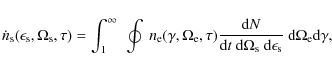
The differential number density of Compton scattered synchrotron photons with the normalised scattered photon energy $\epsilon_{\rm s} = E_{\gamma}/(m_{\rm e} c^2)$ is given by

$\begin{displaymath} \dot{n}_{\rm s}(\epsilon_{\rm s}, \tau) = {c \sigma _T \over... ...}-\gamma ^2 \epsilon\bigr) ~ {\rm d}\gamma ~ {\rm d}\epsilon , \end{displaymath}$

(21)

using the $\delta$ -distribution approximation for inverse Compton scattering introduced by Dermer & Schlickeiser (1993). The limit imposed on the $\gamma$ -integral restricts the scattering to the Thomson regime. Here, we neglect effects due to stimulated synchrotron self-Compton emission and absorption, as well as higher order synchrotron self-Compton scattering. Higher order contributions are expected to be small because they operate in the extreme Klein-Nishina limit where inverse Compton losses are much reduced (Schlickeiser 2009) and, therefore, are negligible compared to synchrotron and triplet pair production losses. This leads to the synchrotron self-Compton intensity

$\begin{displaymath} I_{\rm c}(\epsilon_{\rm s}, \tau) = R j_{\rm c}(\epsilon_{\r... ...lon_{\rm s}}{4 \pi} \dot{n}_{\rm s}(\epsilon_{\rm s}, \tau) . \end{displaymath}$

(22)

Inserting the relativistic electron distribution (5) into Eq. (21) we obtain

$\displaystyle \dot{n}_{\rm s}^{\rm NL}(\epsilon _{\rm s}, \tau)$	=	$\displaystyle {c \sigma _T q_0 \over 3 \pi \gamma_0^2} (1 + \tau - \tau_0) H\biggl({\gamma _0\over \sqrt{1 + \tau - \tau_0}}- \epsilon_{\rm s}\biggr)$
		$\displaystyle \times n^{\rm NL}\left({ \epsilon _{\rm s} (1 + \tau - \tau_0)\over \gamma_0^2}, \tau \right) .$	(23)

Equation (22) then yields

$\displaystyle I_{\rm c}(\epsilon _{\rm s}, \tau)$	=	$\displaystyle {c \sigma _T h R q_0 \epsilon_{\rm s} \over 12 \pi ^2 \gamma_0^2}... ...au_0)H\biggl({\gamma _0\over \sqrt{1 + \tau - \tau_0}}- \epsilon_{\rm s}\biggr)$
		$\displaystyle \times n^{\rm NL}\left({ \epsilon _{\rm s} (1 + \tau - \tau_0)\over \gamma_0^2}, \tau \right) .$	(24)

Making use of the synchrotron photon number densities (19) and (20) we find for the synchrotron self-Compton intensity

		$\displaystyle I_{\rm c}\biggl(\epsilon _{\rm s}\leq \frac{\epsilon _t \gamma_0^... ...a_0^4 \epsilon_0^2 \omega_1^{5/3}} \epsilon_{\rm s}^2 (1 + \tau - \tau_0)^{3/2}$
		$\displaystyle \hspace*{4mm}\times H\biggl({\gamma _0 \over \sqrt{1 + \tau - \ta... ...lon_{\rm s} \over \epsilon_0 \gamma _0^2}(1 + \tau - \tau_0)^{9/4} \biggr]^{-1}$	(25)

and

		$\displaystyle I_{\rm c}(\epsilon_{\rm s} > \frac{\epsilon _t \gamma_0^2}{1 + \t... ...amma_0^{2/3} \epsilon_0^{1/3}} \epsilon_{\rm s}^{1/3} (1 + \tau - \tau_0)^{1/2}$
		$\displaystyle \hspace*{4mm} \times H\biggl({\gamma _0 \over \sqrt{1 + \tau - \t... ...ac{\epsilon_{\rm s} (1 + \tau - \tau_0)^{9/4}}{\epsilon_0 \gamma_0^2}\biggr)} ,$	(26)

respectively.

We introduce a strictly decreasing function to simplify the following expressions and relations

$\begin{displaymath}\epsilon_k(\tau) = \frac{\epsilon_t(\tau) \gamma_0^2}{1 + \tau - \tau_0}\cdot \end{displaymath}$

(27)

For times $\tau - \tau_0$ less and greater than $\omega^{- 20/33}_1 \equiv \tau_1$ (Appendix A) we obtain, analytically continuating the $\tau$ -domain,

$\begin{displaymath}\epsilon_k(\tau - \tau_0 \leq \tau_1) = \frac{\epsilon_0 \omega_1 \gamma_0^2}{(1 + \tau - \tau_0)^{3/5}} \end{displaymath}$

(28)

and

$\begin{displaymath}\epsilon_k(\tau - \tau_0 > \tau_1) = \frac{\epsilon_0 \gamma_... ...( \frac{3}{2} \omega_1^{5/3} (\tau - \tau_0)^{11/4} \biggr)} , \end{displaymath}$

(29)

using Eqs. (A.2) and (A.5).

6 Synchrotron self-Compton fluences

We discuss the synchrotron self-Compton fluence distribution described by the time-integrated synchrotron self-Compton intensity (22)

$\begin{displaymath} F(\epsilon _{\rm s}) = \int_{t_0}^\infty I_{\rm c}(\epsilon_... ...\tau_0}^\infty I_{\rm c}(\epsilon_{\rm s}, \tau) ~ {\rm d}\tau \end{displaymath}$

(30)

in two scattered photon energy ranges: for energies $\epsilon_{\rm s} > \epsilon _k(\tau_0) = \epsilon_{k, {\rm max}}$ only the optically thin synchrotron photon distribution (26) contributes, whereas at lower energies, $\epsilon_{\rm s} \le \epsilon _k(\tau_0) = \epsilon_{k, {\rm max}}$ , both the optically thin and thick parts (25) and (26) of the synchrotron photon distribution have to be taken into account.

6.1 High scattered photon energies

For energies $\epsilon_{\rm s} > \epsilon _k(\tau_0) = \epsilon_{k, {\rm max}}$ only Eq. (26) contributes, so that

		$\displaystyle F\bigl(\epsilon_{\rm s} > \epsilon _k(\tau_0)\bigr) = {R \sigma _... ..._0^{1/3}} \epsilon_{\rm s}^{1/3} \int_{\tau_0}^\infty (1 + \tau - \tau_0)^{1/2}$
		$\displaystyle \hspace*{4mm}\times \exp{\biggl(-{\epsilon_{\rm s} (1 + \tau - \t... ...{\gamma_0 \over \sqrt{1 + \tau - \tau_0}}-\epsilon_{\rm s}\biggr) {\rm d}\tau .$	(31)

Substituting $z = 1 + \tau - \tau_0$ yields

$\begin{displaymath} F\bigl(\epsilon_{\rm s} > \epsilon _k(\tau_0)\bigr) = \frac{... ... s} z^{9/4} \over \epsilon_0 \gamma_0^2}\biggr)} ~ {\rm d}z , \end{displaymath}$

(32)

where

$\begin{displaymath} F_0 \equiv {R \sigma _T I_0 \over 6 \pi A_0 \gamma _0^{1/2}} \cdot \end{displaymath}$

(33)

We obtain with the new variable $y= \epsilon_{\rm s}^2 z/\gamma_0^2$

$\displaystyle % F\bigl(\epsilon_{\rm s} > \epsilon _k(\tau_0)\bigr) = \frac{F_0... ...a_0^{5/2} y^{9/4} \over \epsilon_0 \epsilon_{\rm s}^{7/2}}\biggr)} ~ {\rm d}y .$

(34)

Defining s = y^9/4 and $\epsilon_{\rm f} \equiv \gamma_0^{5/7}/\epsilon_0^{2/7}$ the fluence reads

$\displaystyle F\bigl(\epsilon_{\rm s} > \epsilon _k(\tau_0)\bigr) = \frac{4 F_0... ...[ \frac{\epsilon_{\rm f}}{\epsilon_{\rm s}}\biggr]^{7/2} s\biggr)} ~ {\rm d}s .$

(35)

For high scattered photon energies, $\epsilon_{\rm f} < \epsilon_{\rm s} \leq \gamma_0$ , the argument of the exponential function in the integral of Eq. (35) becomes very small for all values of s yielding approximately

$\displaystyle % F\bigl(\epsilon_{\rm s} > \epsilon_{\rm f} > \epsilon _k(\tau_0)\bigr)$	=	$\displaystyle \frac{4 F_0 \epsilon_{\rm f}^{7/6}}{9 \epsilon_{\rm s}^{8/3}} \int_{(\epsilon_{\rm s} / \gamma_0)^{9/2}}^{1} s^{-1/3} ~ {\rm d}s$
	=	$\displaystyle \frac{2 F_0 \epsilon_{\rm f}^{7/6}}{3 \epsilon_{\rm s}^{8/3}} \biggl( 1 - \biggl[ \frac{\epsilon_{\rm s}}{\gamma_0}\biggr]^3\biggr)\cdot$	(36)

For scattered photon energies $\epsilon _k(\tau_0)\leq \epsilon _{\rm s} < \epsilon_{\rm f}$ we substitute $v = s (\epsilon_{\rm f}/\epsilon_{\rm s})^{7/2}$ to obtain for the fluence (35)

$\displaystyle % F\bigl(\epsilon_{\rm f} > \epsilon_{\rm s} \geq \epsilon _k(\tau_0)\bigr)$	=	$\displaystyle \frac{4 F_0}{9 \epsilon_{\rm s}^{1/3} \epsilon_{\rm f}^{7/6}} \in... ...{(\epsilon_{\rm f} / \epsilon_{\rm s})^{7/2}} v^{-1/3} {\rm e}^{- v} ~ {\rm d}v$
	=	$\displaystyle \frac{4 F_0}{9 \epsilon_{\rm s}^{1/3} \epsilon_{\rm f}^{7/6}} \Ga... ...^{9/2}}, \biggl[\frac{\epsilon_{\rm f}}{\epsilon_{\rm s}} \biggr]^{7/2} \Biggr)$	(37)

in terms of the generalised incomplete gamma function $\Gamma (\cdot, \cdot, \cdot)$ . The second argument of the generalised incomplete gamma function $\epsilon_{\rm f}^{7/2} \epsilon_{\rm s}/\gamma_0^{9/2}$ is much smaller than unity for all scattered photon energies $\epsilon _k(\tau_0)\leq \epsilon _{\rm s} < \epsilon_{\rm f}$ , while the third argument $(\epsilon_{\rm f}/\epsilon_{\rm s})^{7/2}$ is much larger than unity, so that the generalised incomplete gamma function can be asymptotically expanded (Abramowitz & Stegun 1972) leading to the approximated fluence distribution

$\begin{displaymath}F\bigl(\epsilon_{\rm f} > \epsilon_{\rm s} \geq \epsilon _k(\... ... \epsilon_{\rm f}^{7/6}} \Gamma\biggl( \frac{2}{3}\biggr)\cdot \end{displaymath}$

(38)

6.2 Low scattered photon energies

For low scattered photon energies, $\epsilon_{\rm s} \leq \epsilon_k(\tau_0) = \epsilon_{k, {\rm max}}$ , Eqs. (25) and (26) contribute to the spectral fluence. Starting with the scattered photon range $\epsilon_k(\tau_1) \leq \epsilon_{\rm s} \leq \epsilon_k(\tau_0)$ we find, substituting as before

		$\displaystyle F\bigl(\epsilon_k(\tau_1) \leq \epsilon_{\rm s} \leq \epsilon_k(\tau_0)\bigr) = \frac{1}{2 A_0 q_0 \gamma_0^2}$
		$\displaystyle \hspace*{4mm} \times \Biggl(\int_{\tau_0}^{\infty} I_{\rm c}(\eps... ...igl( \epsilon_k(\tau - \tau_0 \leq \tau_1) - \epsilon_{\rm s}\bigr) {\rm d}\tau$
		$\displaystyle \hspace*{4mm} + \int_{\tau_0}^{\infty} I_{\rm c}(\epsilon_{\rm s}... ...silon_{\rm s} - \epsilon_k(\tau - \tau_0 \leq \tau_1)\bigr) {\rm d}\tau \Biggr)$
		$\displaystyle \hspace*{4mm} = \frac{R \sigma_T I_0}{6 \pi A_0 \gamma_0^2} \Bigg... ...\frac{3 \epsilon_{\rm s} z^{9/4}}{2 \gamma_0^2 \epsilon_0}\biggr]^{-1} {\rm d}z$
		$\displaystyle \hspace*{4mm} + \frac{\epsilon_{\rm s}^{1/3}}{\gamma_0^{2/3} \eps... ...c{\epsilon_{\rm s} z^{9/4}}{\gamma_0^2 \epsilon_0}\biggr)} ~ {\rm d}z \Biggr) .$	(39)

The integrand of the first integral can be approximated within the domain of integration by

$\begin{displaymath}z^{3/2} \biggl[1 + \frac{3 \epsilon_{\rm s}}{2 \gamma_0^2 \epsilon_0} z^{9/4} \biggr]^{-1} \approx z^{3/2} . \end{displaymath}$

(40)

Using this approximation and the previous substitutions we obtain for the fluence

		$\displaystyle F\bigl(\epsilon_k(\tau_1) \leq \epsilon_{\rm s} \leq \epsilon_k(\... ...frac{\epsilon_0 \omega_1 \gamma_0^2}{\epsilon_{\rm s}}\biggr]^{25/6} - 1\biggr)$
		$\displaystyle \hspace*{4mm}+ \frac{4 \epsilon_0^{1/3} \gamma_0^{2/3}}{9 \epsilo... ...biggl[\frac{\epsilon_{\rm f}}{\epsilon_{\rm s}}\biggr]^{7/2}\biggr)\Biggr)\cdot$	(41)

The dominant contribution to the fluence again represents synchrotron photons from the optically thin part of the synchrotron spectrum

$\begin{displaymath}F\bigl(\epsilon_k(\tau_1) \leq \epsilon_{\rm s} \leq \epsilon... ...\epsilon_{\rm f}^{7/6}} \Gamma\biggl( \frac{2}{3}\biggr)\cdot \end{displaymath}$

(42)

For scattered photon energies $\epsilon_{\rm s} < \epsilon_k(\tau_1)$ the fluence reads

		$\displaystyle F\bigl(\epsilon_{\rm s} < \epsilon_k(\tau_1)\bigr) = \frac{1}{2 A_0 q_0 \gamma_0^2}$
		$\displaystyle \hspace*{4mm}\times \Biggl(\int_{\tau_0}^{\infty} I_{\rm c}(\epsi... ...H\bigl( \epsilon_k(\tau - \tau_0 > \tau_1) - \epsilon_{\rm s}\bigr) {\rm d}\tau$
		$\displaystyle \hspace*{4mm}+ \int_{\tau_0}^{\infty} I_{\rm c}(\epsilon_{\rm s} ... ...psilon_{\rm s} - \epsilon_k(\tau - \tau_0 > \tau_1)\bigr) {\rm d}\tau \Biggr) .$	(43)

Using the substitutions and approximations applied before we obtain

$\begin{displaymath}F\bigl(\epsilon_{\rm s} < \epsilon_k(\tau_1)\bigr) = \frac{4 ... ...\epsilon_{\rm f}^{7/6}} \Gamma\biggl( \frac{2}{3}, 1\biggr) . \end{displaymath}$

(44)

Again the contribution representing the optically thick part of the spectrum is negligibly small compared to the contribution representing the optically thin part, demonstrating that the fluence distribution $\propto$ $\epsilon_{\rm s}^{-1/3}$ also holds in the scattered photon energy range $\epsilon_{\rm s} < \epsilon_k(\tau_1)$ .

$\begin{figure} \par\includegraphics[width=7.8cm,clip]{11250fg1.eps} \end{figure}$	Figure 1: Time-averaged spectrum observed from PKS 2155-304 on MJD 53944. The dashed line represents the fit for the linear cooling case (Schlickeiser & Röken 2008), whereas the solid curve illustrates the fit for the nonlinear cooling case.
Open with DEXTER

6.3 AIC model selection test

Figure 1 shows the linear (dashed curve) and nonlinear (solid curve) fits to the time-averaged spectrum observed from PKS 2155-304 on MJD 53944 (Aharonian et al. 2007). For the generation of these fits we first had to transform the calculated fluence distributions from the comoving frame into the observer frame (asterisked quantities)

$\begin{displaymath}F^{*}(\epsilon_{\rm s}^{*}) = D^3 F(\epsilon_{\rm s}) = D^3 F(\epsilon_{\rm s}^{*}/D) , \end{displaymath}$

(45)

followed by the construction of the linear model parametric function

$\begin{displaymath} F_{\rm L}^{*}(\epsilon_{\rm s}^{*}) = P_{{\rm L}, 1} \frac{1... ...\frac{\epsilon_{\rm s}^{*}}{P_{{\rm L}, 3}}\bigr)^{7/4}\Bigr)} \end{displaymath}$

(46)

(results from the linear synchrotron self-Compton fluence distribution in the $\delta$ -distribution approximation (Schlickeiser & Röken 2008)) with the parameters $P_{{\rm L}, 1} = D^{11/4} F_0 / \epsilon_{\rm f}^{3/4}$ , $P_{{\rm L}, 2} = D \gamma_0$ and $P_{{\rm L}, 3} = D \epsilon_{\rm f}$ and the nonlinear model parametric function

$\begin{displaymath} F_{\rm NL}^{*}(\epsilon_{\rm s}^{*}) = P_{{\rm NL}, 1} \frac... ...frac{\epsilon_{\rm s}^{*}}{P_{{\rm NL}, 3}}\bigr)^{7/3}\Bigr)} \end{displaymath}$

(47)

with $P_{{\rm NL}, 1} = D^{10/3} F_0 / \epsilon_{\rm f}^{7/6}$ , $P_{{\rm NL}, 2} = D \gamma_0$ and $P_{{\rm NL}, 3} = D \epsilon_{\rm f}$ from our calculated fluence distributions, which we fitted (3 parameters, 14 degrees of freedom) to the PKS 2155-304 data. Finally we carried out a so-called AIC model selection test (Akaike 1974) that measures the quality of a fit of a statistical model, i.e. the precision and complexity of the model, where the preferred model is that with the smallest AIC value. We found the linear fit with an AIC value of 13.37 and a reduced $\chi^2$ -value of 1.37 to be more consistent with the data than the nonlinear fit with an AIC value of 30.15 and a reduced $\chi^2$ -value of 3.67. The parameters were determined to be $P_{{\rm L}, 1} = 5.5 \times 10^{-10} \pm 1.671 \times 10^{-11}$ , $P_{{\rm L}, 3} = 0.433 \pm 0.017$ and $P_{{\rm NL}, 1} = 1.007 \times 10^{-9} \pm 3.396 \times 10^{-11}$ , $P_{{\rm NL}, 3} = 0.619 \pm 0.03$ . The fits turn out to be independent of the parameters $P_{{\rm L}, 2}$ and $P_{{\rm NL}, 2}$ , because both functions (46) and (47) converge as long as the relation $\epsilon_{\rm s}^{*}/P_2 < 1$ is satisfied, leading always to the parameters listed above. Note that the test was performed for only one specific data record for which the linear fit was found to be the best. To transform this indication into a solid conclusion we have to perform tests on more statistical ensembles.

7 Summary and conclusions

Schlickeiser & Lerche (2007) developed a nonlinear model for the synchrotron radiation cooling of ultra-relativistic particles in powerful non-thermal radiation sources assuming a partition condition between the energy densities of the magnetic field and the relativistic electrons. Here, we used this model in order to calculate the synchrotron self-Compton process in flaring TeV blazars and compared it to the results obtained with the standard linear synchrotron cooling model. For simplicity we chose the case of instantaneously injected monoenergetic relativistic electrons as an example, although other injection scenarios, like the instantaneous injection of power-law distributed electrons (Schlickeiser & Lerche 2008), are also possible. After the nonlinear electron synchrotron cooling, the created synchrotron photons with non-relativistic energies are multiple Thomson scattered off the cooled electrons in the source (synchrotron self-Compton process).

We calculated the optically thin and thick synchrotron radiation intensities as well as the synchrotron photon density distributions in the emission knot as functions of frequency and time. These synchrotron photons serve as target photons in the synchrotron self-Compton process. Using the Thomson approximation of the inverse Compton cross section, we determined the synchrotron self-Compton intensity and fluence for the nonlinear electron cooling. It is shown that the optically thick synchrotron radiation component provides only a negligible contribution to the synchrotron self-Compton quantities at all frequencies and times, as in the linear cooling case. In Appendix B, we extended our calculations to the full Klein-Nishina cross section and obtained additional positive and negative, non-vanishing fluence contributions only in the high-energy regime $\epsilon_{\rm f}^{\rm L, NL} < \epsilon_{\rm s} \leq \gamma_0$ of the scattered photons, e.g. generalised incomplete $\Gamma$ -functions or the new generalised dual hypergeometric functions. Surprisingly, for the special class of electron and synchrotron photon distributions used in this work, these contributions nearly cancel each other out on average, leaving only a small positive fluence contribution (see Figs. B.5 and B.6) which we expected to be due to the consideration of high energy photons in the scattering process. Because of the smallness of the new contribution it can be justified to model the photon spectra by applying the $\delta$ -distribution approximation for the calculation of the differential inverse Compton scattering rate for electron and synchrotron densities of the form (B.15), (B.16) as well as (B.23) and (B.24).

Finally, we compared the linear to the nonlinear fluence distribution, fitting both to the observed TeV fluence spectrum of PKS 2155-304 on MJD 53944 and performed a statistical quality-of-fit test (AIC test). For this particular data record, we found the linear model to be more appropriate than the nonlinear. Actually, with the formalism we presented here, we cannot fit the entire spectral energy distribution because we neglect the synchrotron self-Compton component of energy losses and only discuss the synchrotron one. Therefore, Schlickeiser (2009) has shown that synchrotron self-Compton cooling is an alternative nonlinear cooling process that can be handled analytically as long as it operates in the Thomson limit. Nonetheless, the excellent agreement of both linear and nonlinear synchrotron self-Compton fluence spectra with the observation of the gamma-ray flare of PKS 2155-304 supports the injection scenario of monoenergetic electrons by the relativistic pickup process.

Acknowledgements

This work was partially supported by the German Ministry for Education and Research (BMBF) through Verbundforschung Astroteilchenphysik grant 05 CH5PC1/6 and the Deutsche Forschungsgemeinschaft through grant Schl 201/16-2.

Appendix A: Synchrotron optical depth and photon spectra

A.1 Optical depth

The synchrotron emission of ultra-relativistic electrons is optically thin for frequencies and times satisfying the condition $D(\omega, \tau) \leq 1$ and optically thick for $D(\omega, \tau) > 1$ . The transition occurs at the frequency $\omega_t(\tau)$ defined by $D(\omega, \tau) = 1$ . For $\tau - \tau_0 \ll 1$ (and its analytical continuation) the optical depth (15) reduces to

$\begin{displaymath} D(\omega, \tau - \tau_0 \leq 1) \simeq \biggl(\frac{\omega_1}{\omega}\biggr)^{5/3} (1 + \tau - \tau_0)^{2/3} \end{displaymath}$

(A.1)

as long as $\tau - \tau_0\leq \omega^{-4/5}$ . In this range the transition frequency reads

$\begin{displaymath} \omega_t(\tau - \tau_0 \leq \omega^{-4/5}) \simeq \omega_1 (1 + \tau - \tau_0)^{2/5} . \end{displaymath}$

(A.2)

In the domain $\tau - \tau_0 \gg 1$ (and its analytical continuation) the optical depth simplifies to

$\displaystyle D(\omega, \tau - \tau_0 > 1) \simeq \biggl(\frac{\omega_1}{\omega... ...\tau - \tau_0)^{5/4}\biggr) \exp{ \Bigl(- \omega (\tau - \tau_0)^{5/4} \Bigr)}.$

(A.3)

Substituting $z = \omega (\tau - \tau_0)^{5/4}$ and expanding asymptotically for z > 1 as well as for $z \leq 1$ we find

D(z)	=	$\displaystyle \omega^{5/3}_1 \omega^{-11/5} z^{8/15} \biggl( 1 + \frac{3}{2} z\biggr) {\rm e}^{-z}$
	$\textstyle \simeq$	$\displaystyle \omega_1^{5/3} \omega^{-11/5} \left\{ \begin{array}{ll} z^{8/15},... ... \displaystyle{\frac{3}{2} z^{23/15} {\rm e}^{-z}} ,& z > 1 \end{array}\right.$	(A.4)

with the proper transition frequency

$\displaystyle \omega_t(\tau) \simeq \left\{\begin{array}{ll} \omega_1 (\tau - \... ...tau - \tau_0)^{5/4}}} ,& \tau - \tau_0 > \omega_1^{-20/33} \end{array} .\right.$

(A.5)

In Fig. A.1, we present the time-dependence of the transition frequency. For small times $\tau - \tau_0 \leq 1$ , the transition frequency is constant at the value $\omega_1$ . After this, it increases linearly to its maximum value $\omega_1^{25/33}$ at $\tau - \tau_0 = \omega_1^{-20/33}$ , followed by a decrease proportional to $\tau^{-5/4}$ at times $\tau - \tau_0 > \omega_1^{-20/33}$ .

$\begin{figure} \par\includegraphics[width=6.5cm,clip]{11250fg2.eps} \end{figure}$	Figure A.1: Normalised synchrotron transition frequency $\omega _t$ as a function of time $\tau$ in the nonlinear cooling case plotted for $\omega _1 = 10^{-15}$ . The instantaneous injection of monoenergetic ultra-relativistic electrons occurred at $\tau _0 = 0$ .
Open with DEXTER

A.2 Synchrotron spectra

According to Eq. (11), the synchrotron intensity in the optically thick frequency domain $\omega \leq \omega_t$ is given by

$\displaystyle I(\omega \leq \omega_t, \tau) \simeq {j(\omega, \tau) R \over D(\... ...- \tau_0)^{1/2} \Bigl(1 + \frac{3}{2} \omega (1 + \tau - \tau_0)^{5/4}\Bigr)} ,$

(A.6)

where $I_0 \equiv a_0 P_0 q_0 R \nu_0/(4 \pi)$ . In the optically thin frequency interval, $\omega > \omega_t$ , we obtain

$\displaystyle I(\omega > \omega_t, \tau)$	$\textstyle \simeq$	$\displaystyle j(\omega, \tau) R$
	=	$\displaystyle I_0 \omega^{1/3} (1 \!+\! \tau - \tau_0)^{1/6} \exp{\bigl(-\omega (1 \!+\! \tau - \tau_0)^{5/4} \bigr)}\cdot$	(A.7)

In Fig. A.2, we show the intensity distribution as a function of the frequency $\omega$ at various times $\tau = 0, 10^4, 10^9$ and 10¹¹. Consequently, the transition intensity reads

$\displaystyle I_{\rm trans}(\tau)$	=	$\displaystyle I(\omega_t,\tau)$
	=	$\displaystyle I_0 \omega^{-5/3}_1 {\omega^2_t\over (1 + \tau - \tau_0)^{1/2} \Bigl[1 + \frac{3}{2} \omega_t (1 + \tau - \tau_0)^{5/4} \Bigr]}\cdot$	(A.8)

Applying the transition frequencies (A.2) and (A.5) we obtain for the transition intensity at normalised times $\tau - \tau_0 \leq \omega^{-20/33}_1$

$\begin{displaymath} I_{\rm trans}(\tau - \tau_0 \leq \omega^{-20/33}_1) \simeq I... ...} \over 1 + \frac{3}{2} \omega_1 (1 + \tau - \tau_0)^{33/20}}, \end{displaymath}$

(A.9)

whereas at times $\tau - \tau_0 > \omega^{-20/33}_1$ the result is

$\begin{displaymath}I_{\rm trans}(\tau - \tau_0 > \omega^{-20/33}_1) \simeq {2 I_... ...}_1 (\tau - \tau_0)^{11/4}\Bigr)}\over (\tau - \tau_0)^3}\cdot \end{displaymath}$

(A.10)

At small times $\tau - \tau_0 \leq 1$ the transition intensity turns out to be

$\begin{displaymath}I_{\rm trans}(\tau - \tau_0 \leq 1) \simeq I_0 \omega_1^{1/3} . \end{displaymath}$

(A.11)

The time-dependence of the transition intensity is presented in Fig. A.3.

$\begin{figure} \par\includegraphics[width=6.5cm,clip]{11250fg3.eps} \end{figure}$	Figure A.2: Synchrotron intensity distribution as a function of frequency $\omega$ at different times $\tau = 0$ (solid curve), $\tau = 10^4$ (dash-dotted curve), $\tau = 10^9$ (dotted curve) and $\tau = 10^{11}$ (dashed curve). The injection occurred at $\tau _0 = 0$ with the parameter $\omega _1 = 10^{-15}$ .
Open with DEXTER

$\begin{figure} \par\includegraphics[width=6.5cm,clip]{11250fg4.eps} \end{figure}$	Figure A.3: Synchrotron transition intensity $I_{\rm trans}/I_0$ as a function of time $\tau$ plotted for $\omega _1 = 10^{-15}$ at the injection time $\tau _0 = 0$ .
Open with DEXTER

Appendix B: Synchrotron self-Compton scattering with the full Klein-Nishina cross section

B.1 The process of synchrotron self-Compton emission

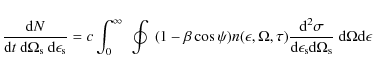
The differential inverse Compton scattering rate $\dot n_{\rm s}$ in a coordinate system comoving with the radiation source (unprimed quantities) is given by (Dermer et al. 1992)

$\begin{displaymath} \dot n_{\rm s}(\epsilon_{\rm s}, \Omega_{\rm s}, \tau) = \in... ...{\rm d}\epsilon_{\rm s}}~ {\rm d}\Omega_{\rm e} {\rm d}\gamma, \end{displaymath}$

(B.1)

where $\gamma$ is the normalised energy of a single electron, $\epsilon _{\rm s}$ the normalised energy of a scattered photon, N the scattered photon number, $n_{\rm e}$ the differential electron density and $\Omega_{\rm s}$ and $\Omega_{\rm e}$ are the solid angles of the scattered photons and electrons, respectively. The single electron differential scattering rate reads

$\begin{displaymath}\frac{{\rm d}N}{{\rm d}t ~ {\rm d}\Omega_{\rm s} ~ {\rm d}\ep... ...{\rm s} {\rm d}\Omega_{\rm s}} ~ {\rm d}\Omega {\rm d}\epsilon \end{displaymath}$

(B.2)

with the normalised energy of an incoming photon $\epsilon$ , the differential synchrotron photon density n and $\psi = \angle \bigl(\vec v_{\rm e}, \vec k_{\rm ph} \bigr)$ . $\vec v_{\rm e}$ is the velocity of the electron and $\vec k_{\rm ph}$ is the wave vector of the incoming photon. The differential Klein-Nishina cross section ${\rm d}^2\sigma/({\rm d}\epsilon_{\rm s} {\rm d}\Omega_{\rm s})$ has the most compact form in the electron rest frame (primed quantites) (Jauch & Rohrlich 1976)

$\begin{displaymath}\frac{{\rm d}^2\sigma}{{\rm d}\epsilon'_{\rm s} {\rm d}\hat \... ...'}\biggr) \delta\bigl(\epsilon'_{\rm s} - \epsilon'_0 \bigr) , \end{displaymath}$

(B.3)

where

$\begin{displaymath}\epsilon'_0 = \frac{\epsilon'}{1 + \epsilon'(1 - \cos{\chi'})} \end{displaymath}$

(B.4)

and $\chi = \angle \bigl(\vec k_{\rm s}, \vec k_{\rm ph} \bigr)$ with the wave vector $\vec k_{\rm s}$ of the scattered photon. We assume isotropic electron and photon distributions in the comoving frame. Hence, the differential Compton scattering rate does not depend on the direction of the outgoing photons, so (B.1) can be reduced to

$\begin{displaymath}\dot n_{\rm s}(\epsilon_{\rm s}, \tau) = \int^{\infty}_1 ~ n_... ...{\rm d}N}{{\rm d}t ~ {\rm d}\epsilon_{\rm s}}~ {\rm d}\gamma . \end{displaymath}$

(B.5)

Following the paper of Arbeiter et al. (2005) we can write

		$\displaystyle \frac{{\rm d}N}{{\rm d}t ~ {\rm d}\epsilon_{\rm s}} \simeq \frac{... ...\delta(\epsilon'_{\rm s} - \epsilon'_0) \frac{\epsilon'^{3}_{\rm s}}{\epsilon'}$
		$\displaystyle \times \biggl( \frac{\epsilon'}{\epsilon'_{\rm s}} + \frac{\epsil... ...ma \epsilon - \epsilon') ~ {\rm d}\cos{\chi'} {\rm d}\epsilon' {\rm d}\epsilon,$	(B.6)

where $H(\cdot)$ denotes the Heaviside step function. Using the so-called head-on approximation (Arbeiter 2005) and $\epsilon_{\rm s} = \gamma \epsilon'_{\rm s} \bigl(1 - \beta \cos{(\chi')} \bigr)$ we obtain for the high-energy regime $\epsilon \ll \epsilon_{\rm s} \leq 4 \epsilon \gamma^2/(1 + 4 \epsilon \gamma)$ (Jones 1967; Blumenthal & Gould 1970)

$\displaystyle \frac{{\rm d}N}{{\rm d}t ~ {\rm d}\epsilon_{\rm s}}$	$\textstyle \simeq$	$\displaystyle \frac{2 \pi r_0^2 c}{\gamma^2} \int^{\infty}_0~ \frac{n(\epsilon,... ...gl(1 - \Lambda(\epsilon, \epsilon_{\rm s})\bigr) H(\epsilon_{\rm s} - \epsilon)$
		$\displaystyle \times \biggl( \bigl(1 - \Lambda(\epsilon, \epsilon_{\rm s})\bigr... ...(\epsilon, \epsilon_{\rm s}) \bigl[ 1 + \epsilon_{\rm s} \epsilon \bigr] \Bigr)$
		$\displaystyle + 2 \Lambda(\epsilon, \epsilon_{\rm s}) \ln{\bigl(\Lambda(\epsilon, \epsilon_{\rm s}) \bigr)} \biggr) ~ {\rm d}\epsilon ,$	(B.7)

where $\Lambda(\epsilon, \epsilon_{\rm s}) = \epsilon_{\rm s}/(4 \gamma^2 \epsilon (1 - \epsilon_{\rm s}/\gamma))$ , and for the low-energy regime $\epsilon/4 \gamma^2 \leq \epsilon_{\rm s} \ll \epsilon$

$\begin{displaymath} \frac{{\rm d}N}{{\rm d}t ~ {\rm d}\epsilon_{\rm s}} \approx ... ...ma^2 \epsilon_{\rm s}}{\epsilon} - 1\biggr)~ {\rm d}\epsilon . \end{displaymath}$

(B.8)

In the following calculations of the synchrotron self-Compton intensities and fluences we disregard (B.8) and only use the dominant contribution (B.7) of the differential scattering rate for a single electron.

B.2 Linear and nonlinear synchrotron self-Compton intensities

Neglecting effects due to stimulated synchrotron self-Compton emission and absorption the synchrotron self-Compton intensity reads

$\begin{displaymath} I_{\rm c}(\epsilon_{\rm s}, \tau) = R j_{\rm c}(\epsilon_{\r... ...silon_{\rm s}}{4 \pi} \dot n_{\rm s}(\epsilon_{\rm s}, \tau) , \end{displaymath}$

(B.9)

where $j_{\rm c}(\epsilon_{\rm s}, \tau)$ is the spontaneous synchrotron emission coefficient and R the radius of the source. For the differential scattering rate $\dot n_{\rm s}(\epsilon_{\rm s}, \tau)$ we use the dominant high-energy contribution (B.7) yielding

		$\displaystyle \dot n_{\rm s}(\epsilon_{\rm s}, \Omega_{\rm s}, \tau) = 2 \pi r_... ..., \tau) \frac{1}{\gamma^2} \int^{\infty}_0 ~ \frac{n(\epsilon, \tau)}{\epsilon}$
		$\displaystyle \hspace*{4mm} \times H\bigl(1 - \Lambda(\epsilon, \epsilon_{\rm s... ...psilon, \epsilon_{\rm s})\bigr) \Bigl(1 + 2 \Lambda(\epsilon, \epsilon_{\rm s})$
		$\displaystyle \hspace*{4mm} \times \bigl[ 1 + \epsilon_{\rm s} \epsilon \bigr] ... ...da(\epsilon, \epsilon_{\rm s}) \bigr)} \biggr) ~ {\rm d}\epsilon {\rm d}\gamma.$	(B.10)

Consequently, we have to distinguish between the three cases $\epsilon \Lambda(\epsilon, \epsilon_{\rm s}) < \epsilon_{\rm s} < \epsilon_t$ , $\epsilon_t < \epsilon \Lambda(\epsilon, \epsilon_{\rm s}) < \epsilon_{\rm s}$ and $\epsilon \Lambda(\epsilon, \epsilon_{\rm s}) < \epsilon_t < \epsilon_{\rm s}$ , where $\epsilon_t$ is the transition energy from the optically thin to the optically thick synchrotron emission regime. For the linear cooling case the transition energy reads (Schlickeiser & Röken 2008)

$\begin{displaymath}\epsilon_t^{\rm L} = \epsilon_0 \left\{\begin{array}{ll} \om... ...au > \bigl(\omega_1^{{\rm L}}\bigr)^{-1/3} \end{array}\right. \end{displaymath}$

(B.11)

and for the nonlinear electron cooling case

$\begin{displaymath}\epsilon_t^{\rm NL} = \epsilon_0 \left\{\begin{array}{ll} \o... ... > \bigl(\omega_1^{\rm NL}\bigr)^{-20/33}. \end{array}\right. \end{displaymath}$

(B.12)

Here, we discuss only the case $\epsilon_t < \epsilon \Lambda(\epsilon, \epsilon_{\rm s}) < \epsilon_{\rm s}$ as explained below in Appendix B.3. Therefore, we define the functions

$\begin{displaymath}\epsilon_k^{\rm L}(\tau) = \frac{4 \gamma_0^2 \epsilon_0 \omega_1^{\rm L}}{1 + \tau} \end{displaymath}$

(B.13)

and

$\begin{displaymath}\epsilon_k^{\rm NL}(\tau) = \frac{4 \gamma_0^2 \epsilon_0 \omega_1^{\rm NL}}{(1 + \tau)^{3/5}} \end{displaymath}$

(B.14)

with $\omega_1^{\rm L, NL} = (a_0 P_0 q_0 R/(6 \pi \nu_{{\rm L, NL}} m_{\rm e} \gamma_0^5))^{3/5}$ , $\nu_{\rm L} = 3 e B/(4 \pi m_{\rm e} c)$ and $\nu_{\rm NL} = 3 e ~ \sqrt{e_B q_0 \gamma_0/(2 \pi m_{\rm e})}$ .

B.2.1 Linear electron cooling

To compute the linear differential scattering rate we insert the linear differential electron density (Schlickeiser & Lerche 2007)

$\begin{displaymath} n^{\rm L}_{\rm e}(\gamma, \tau) = q_0 H\bigl(\gamma_0 - \gam... ...bigr) \delta \biggl(\gamma - \frac{\gamma_0}{1 + \tau} \biggr) \end{displaymath}$

(B.15)

and the linear synchrotron photon density

$\begin{displaymath} n^{\rm L}(\epsilon, \tau) = \frac{4 \pi I_0}{h c \epsilon^{1... ...exp{\biggl(- \frac{\epsilon}{\epsilon_0} (1 + \tau)^2 \biggr)} \end{displaymath}$

(B.16)

into Eq. (B.10). Then we obtain

		$\displaystyle \dot n^{\rm L}_{\rm s}(\epsilon_{\rm s}, \tau) = n_0 (1 + \tau)^{... ...r \Lambda_{\rm L}(\epsilon_{\rm s}, \tau)}^{\epsilon_{\rm s}} ~ \epsilon^{-5/3}$

		$\displaystyle \hspace*{4mm}\times {\rm e}^{- f(\tau) \epsilon} \biggl( \bigl(1 ... ...lon, \epsilon_{\rm s}, \tau) \bigl[ 1 + \epsilon_{\rm s} \epsilon \bigr] \Bigr)$

		$\displaystyle \hspace*{4mm}+ 2 \Lambda_{\rm L}(\epsilon, \epsilon_{\rm s}, \tau... ...mbda_{\rm L}(\epsilon, \epsilon_{\rm s}, \tau) \bigr)} \biggr)~ {\rm d}\epsilon$	(B.17)

with the constant $n_0 = 8 \pi^2 r_0^2 q_0 I_0/(h \epsilon_0^{1/3} \gamma_0^2)$ and the functions $f(\tau) = (1 + \tau)^2/\epsilon_0$ , $\Lambda_{\rm L}(\epsilon, \epsilon_{\rm s}, \tau) = \epsilon_{\rm s} (1 + \tau)^2/(4 \gamma_0^2 \epsilon (1 - \epsilon_{\rm s} (1 + \tau)/\gamma_0))$ and $\bar \Lambda_{\rm L}(\epsilon_{\rm s}, \tau) \equiv \epsilon \Lambda_{\rm L}(\epsilon, \epsilon_{\rm s}, \tau)$ . Transforming ${\rm d}\epsilon$ into ${\rm d}\Lambda_{\rm L}(\epsilon, \epsilon_{\rm s}, \tau)$ we obtain

		$\displaystyle \dot n^{\rm L}_{\rm s}(\epsilon_{\rm s}, \tau) = n_0 (1 + \tau)^{8/3} \bar \Lambda_{\rm L}(\epsilon_{\rm s}, \tau)^{-2/3}$

		$\displaystyle \hspace*{4mm} \times H\biggl(\frac{\gamma_0}{\epsilon_{\rm s}} - ... ...epsilon_{\rm s}}^{1} ~ \Lambda_{\rm L}(\epsilon, \epsilon_{\rm s}, \tau)^{-1/3}$

		$\displaystyle \hspace*{4mm} \times \exp{\biggl(- \frac{f(\tau) \bar \Lambda_{\r... ...+ a_2(\epsilon_{\rm s}, \tau) \Lambda_{\rm L}(\epsilon, \epsilon_{\rm s}, \tau)$

		$\displaystyle \hspace*{4mm} -2 \Lambda_{\rm L}(\epsilon, \epsilon_{\rm s}, \tau... ...m L}(\epsilon, \epsilon_{\rm s}, \tau) \bigr)} \biggr)~ {\rm d}\Lambda_{\rm L},$	(B.18)

where $a_{1/2}(\epsilon_{\rm s}, \tau) = 1 \pm 2 \epsilon_{\rm s} \bar \Lambda_{\rm L}(\epsilon_{\rm s}, \tau)$ . As shown in Appendix B.3 we expect a change of the intensity and fluence behaviours to occur only at high energies, so that (B.18) is sufficiently well approximated by

		$\displaystyle \dot n^{\rm L}_{\rm s}(\epsilon_{\rm s}, \tau) \approx n_0 (1 + \... ...a_1(\epsilon_{\rm s}, \tau) \bar \Lambda_{\rm L}(\epsilon_{\rm s}, \tau)^{-2/3}$

		$\displaystyle \hspace*{4mm} \times H\biggl(\frac{\gamma_0}{\epsilon_{\rm s}} - ... ...epsilon_{\rm s}}^{1} ~ \Lambda_{\rm L}(\epsilon, \epsilon_{\rm s}, \tau)^{-1/3}$

		$\displaystyle \hspace*{4mm} \times \exp{\biggl(-\frac{ f(\tau) \bar \Lambda_{\r... ...ambda_{\rm L}(\epsilon, \epsilon_{\rm s}, \tau)\bigr)~ {\rm d}\Lambda_{\rm L} .$	(B.19)

Substituting $s = f(\tau) \bar \Lambda_{\rm L}(\epsilon_{\rm s}, \tau) \Lambda_{\rm L}(\epsilon, \epsilon_{\rm s}, \tau)^{-1}$ we obtain

$\displaystyle \dot n^{\rm L}_{\rm s}(\epsilon_{\rm s}, \tau)$	=	$\displaystyle n_0 (1 + \tau)^{8/3}a_1(\epsilon_{\rm s}, \tau) f(\tau)^{2/3} H\biggl(\frac{\gamma_0}{\epsilon_{\rm s}} - 1 - \tau \biggr)$

		$\displaystyle \times \int^{f(\tau) \epsilon_{\rm s}}_{f(\tau) \bar \Lambda_{\rm... ...\frac{f(\tau) \bar \Lambda_{\rm L}(\epsilon_{\rm s}, \tau)}{s}\biggr) {\rm d}s,$	(B.20)

which is solved by generalised incomplete Gamma functions

$\displaystyle \dot n^{\rm L}_{\rm s}(\epsilon_{\rm s}, \tau)$	=	$\displaystyle n_0 (1 + \tau)^{8/3}a_1(\epsilon_{\rm s}, \tau) f(\tau)^{2/3} H\biggl(\frac{\gamma_0}{\epsilon_{\rm s}} - 1 - \tau \biggr)$
		$\displaystyle \times \biggl[ \Gamma\biggl(- \frac{2}{3}, f(\tau) \bar \Lambda_{... ...\epsilon_{\rm s} \biggr) - f(\tau) \bar \Lambda_{\rm L}(\epsilon_{\rm s}, \tau)$
		$\displaystyle \times \Gamma\biggl(- \frac{5}{3}, f(\tau) \bar \Lambda_{\rm L}(\epsilon_{\rm s}, \tau), f(\tau) \epsilon_{\rm s} \biggr) \biggr]$
	$\textstyle \approx$	$\displaystyle n_0 (1 + \tau)^{8/3}a_1(\epsilon_{\rm s}, \tau) f(\tau)^{2/3} H\biggl(\frac{\gamma_0}{\epsilon_{\rm s}} - 1 - \tau \biggr)$
		$\displaystyle \times \biggl[ \Gamma\biggl(- \frac{2}{3}, f(\tau) \bar \Lambda_{... ...n_{\rm s}, \tau) \biggr) - f(\tau) \bar \Lambda_{\rm L}(\epsilon_{\rm s}, \tau)$
		$\displaystyle \times \Gamma\biggl(- \frac{5}{3}, f(\tau) \bar \Lambda_{\rm L}(\epsilon_{\rm s}, \tau) \biggr) \biggr].$	(B.21)

We, thus, find the linear synchrotron self-Compton intensity to be

$\displaystyle I^{\rm L}_{\rm c}(\epsilon_{\rm s}, \tau)$	=	$\displaystyle I_0 \epsilon_{\rm s} (1 + \tau)^{8/3} a_1(\epsilon_{\rm s}, \tau) f(\tau)^{2/3} H\biggl(\frac{\gamma_0}{\epsilon_{\rm s}} - 1 - \tau \biggr)$
		$\displaystyle \times \biggl[ \Gamma\biggl(- \frac{2}{3}, f(\tau) \bar \Lambda_{... ...n_{\rm s}, \tau) \biggr) - f(\tau) \bar \Lambda_{\rm L}(\epsilon_{\rm s}, \tau)$
		$\displaystyle \times \Gamma\biggl(- \frac{5}{3}, f(\tau) \bar \Lambda_{\rm L}(\epsilon_{\rm s}, \tau) \biggr) \biggr],$	(B.22)

where $I_0 = h R n_0/(4 \pi)$ . In Figs. B.1 and B.2 we show the linear synchrotron intensity (B.22) as a function of the energy $\epsilon _{\rm s}$ at four different times ( $\tau = 0, 10, 10^2, 10^3$ ) and as a function of the time $\tau$ at four different energies ( $\epsilon_{\rm s} = 10^3, 10^4, 10^5, 10^6$ ).

$\begin{figure} \par\includegraphics[width=6.5cm,clip]{11250fg5.eps} \end{figure}$	Figure B.1: Normalised linear synchrotron intensity $I_{{\rm L}}/I_{0}$ as a function of energy $\epsilon _{\rm s}$ at four different times $\tau = 0$ (solid curve), 10 (dotted curve), 10² (dashed curve) and 10³ (dash-dotted curve).
Open with DEXTER

$\begin{figure} \par\includegraphics[width=6.5cm,clip]{11250fg6.eps} \end{figure}$	Figure B.2: Normalised linear synchrotron light curve $I_{{\rm L}}/I_{0}$ as a function of time $\tau$ at four different energies $\epsilon _{\rm s} = 10^{3}$ (solid curve), 10⁴ (dotted curve), 10⁵ (dashed curve) and 10⁶ (dash-dotted curve).
Open with DEXTER

B.2.2 Nonlinear electron cooling

With the nonlinear differential electron density (Schlickeiser & Lerche 2007)

$\begin{displaymath} n^{\rm NL}_{\rm e}(\gamma, \tau) = q_0 H\bigl(\gamma_0 - \ga... ...delta \biggl(\gamma - \frac{\gamma_0}{\sqrt{1 + \tau}} \biggr) \end{displaymath}$

(B.23)

and the nonlinear synchrotron photon density

$\begin{displaymath} n^{\rm NL}(\epsilon, \tau) = \frac{4 \pi I_0}{h c \epsilon^{... ...\biggl(- \frac{\epsilon}{\epsilon_0} (1 + \tau)^{5/4} \biggr)} \end{displaymath}$

(B.24)

the differential scattering rate reads

$\displaystyle \dot n^{\rm NL}_{\rm s}(\epsilon_{\rm s}, \tau)$	$\textstyle \approx$	$\displaystyle n_0 (1 + \tau)^{7/6} b_1(\epsilon_{\rm s}, \tau) g(\tau)^{2/3} H\biggl(\frac{\gamma^2_0}{\epsilon^2_{\rm s}} - 1 - \tau \biggr)$
		$\displaystyle \times \biggl[ \Gamma\biggl(- \frac{2}{3}, g(\tau) \bar \Lambda_{... ..._{\rm s}, \tau) \biggr) - g(\tau) \bar \Lambda_{\rm NL}(\epsilon_{\rm s}, \tau)$
		$\displaystyle \times \Gamma\biggl(- \frac{5}{3}, g(\tau) \bar \Lambda_{\rm NL}(\epsilon_{\rm s}, \tau) \biggr) \biggr],$	(B.25)

where $g(\tau) = (1 + \tau)^{5/4}/\epsilon_0$ , $\bar \Lambda_{\rm NL}(\epsilon_{\rm s}, \tau) = \epsilon_{\rm s} (1 + \tau)/(4 \gamma_0^2 ( 1 - \epsilon_{\rm s} \sqrt{1 + \tau}/\gamma_0))$ and $b_1(\epsilon_{\rm s}, \tau) = 1 + 2 \epsilon_{\rm s} \bar \Lambda_{\rm NL}(\epsilon_{\rm s}, \tau)$ , applying the same substitutions and approximations as for the linear case. We obtain for the intensity

$\displaystyle I^{\rm NL}_{\rm c}(\epsilon_{\rm s}, \tau)$	=	$\displaystyle I_0 \epsilon_{\rm s} (1 + \tau)^{7/6} b_1(\epsilon_{\rm s}, \tau) g(\tau)^{2/3} H\biggl(\frac{\gamma^2_0}{\epsilon^2_{\rm s}} - 1 - \tau \biggr)$
		$\displaystyle \times \biggl[ \Gamma\biggl(- \frac{2}{3}, g(\tau) \bar \Lambda_{... ..._{\rm s}, \tau) \biggr) - g(\tau) \bar \Lambda_{\rm NL}(\epsilon_{\rm s}, \tau)$
		$\displaystyle \times \Gamma\biggl(- \frac{5}{3}, g(\tau) \bar \Lambda_{\rm NL}(\epsilon_{\rm s}, \tau) \biggr) \biggr].$	(B.26)

In Figs. B.3 and B.4 we present the nonlinear synchrotron intensity (B.26) as a function of the energy $\epsilon _{\rm s}$ at five different times ( $\tau = 0, 10, 10^2, 10^3, 10^5$ ) and as a function of the time $\tau$ at four different energies ( $\epsilon_{\rm s} = 10^3, 10^4, 10^5, 10^6$ ). The different electron synchrotron cooling behaviours can be well observed by comparing for example Figs. B.1 and B.3. We can see that the functional behaviour of the linear intensity distribution at $\tau = 10^2$ fits the behaviour of the nonlinear intensity distribution at later times $\tau > 10^2$ due to a faster linear cooling process.

$\begin{figure} \par\includegraphics[width=6.8cm,clip]{11250fg7.eps} \end{figure}$	Figure B.3: Normalised nonlinear synchrotron intensity $I_{\rm NL}/I_{0}$ as a function of energy $\epsilon _{\rm s}$ at five different times $\tau = 0$ (solid curve), 10 (dotted curve), 10² (dashed curve), 10³ (dash-dotted curve) and 10⁵ (long-dashed curve).
Open with DEXTER

$\begin{figure} \par\includegraphics[width=6.8cm,clip]{11250fg8.eps} \end{figure}$	Figure B.4: Normalised nonlinear synchrotron light curve $I_{\rm NL}/I_{0}$ as a function of time $\tau$ at four different energies $\epsilon _{\rm s} = 10^{3}$ (solid curve), 10⁴ (dotted curve), 10⁵ (dashed curve) and 10⁶ (dash-dotted curve).
Open with DEXTER

B.3 Linear and nonlinear synchrotron self-Compton fluences

By the time-integration of the synchrotron self-Compton intensity (B.9) we obtain the synchrotron self-Compton fluence distribution

$\begin{displaymath} F(\epsilon_{\rm s}) = \int_0^{\infty} ~ I(\epsilon_{\rm s}, t) ~ {\rm d}t . \end{displaymath}$

(B.27)

Here, we only have to examine the range for high scattered photon energies $\epsilon_{\rm s} > 4 \gamma_0^2 \epsilon_0 \omega_1^{\rm L, NL} = \epsilon_{k, {\rm max}}^{\rm L, NL}$ because the action of the full Klein-Nishina cross section becomes apparent in the high-energy scattered photon regime for both the linear and nonlinear case, as shown in the following subsections. For energies much lower than the characteristic energy $\epsilon_{\rm s} < \epsilon_{\rm f}^{\rm L, NL}$ , we find the same solutions as in Schlickeiser & Röken (2008) and as in Sect. 6, leading to the conclusion that the fluence behaviour for $\epsilon_{\rm s} < \epsilon_{k, {\rm max}}^{\rm L, NL}$ is identical to the $\delta$ -distribution-approximated Thomson regime fluence behaviour. Thus, we need only the optically thin synchrotron photon distributions (B.16) and (B.24) for the calculation of the synchrotron self-Compton fluence.

B.3.1 Linear electron cooling

With the linear synchrotron self-Compton intensity distribution (B.22) the synchrotron self-Compton fluence (B.27) reads for $\epsilon_{\rm s} \geq \epsilon^{\rm L}_{k, {\rm max}} = 4 \gamma_0^2 \epsilon_0 \omega^{\rm L}_1$

$\displaystyle F_{\rm L}(\epsilon_{\rm s})$	=	$\displaystyle F^{\rm L}_0 \epsilon_{\rm s} \int_0^{\infty} (1 + \tau)^{8/3} a_1(\epsilon_{\rm s}, \tau) f(\tau)^{2/3}$
		$\displaystyle \times H\biggl(\frac{\gamma_0}{\epsilon_{\rm s}} - 1 - \tau \bigg... ...ggl(- \frac{2}{3}, f(\tau) \bar \Lambda_{\rm L}(\epsilon_{\rm s}, \tau) \biggr)$
		$\displaystyle - f(\tau) \bar \Lambda_{\rm L}(\epsilon_{\rm s}, \tau) \Gamma\big... ...au) \bar \Lambda_{\rm L}(\epsilon_{\rm s}, \tau) \biggr) \biggr]~ {\rm d}\tau ,$	(B.28)

where $F^{\rm L}_0 = h R n_0/(4 \pi D_0 \gamma_0)$ . We start with the computation of the fluence contribution for the first summand of function $a_1(\epsilon_{\rm s}, \tau)$ . Substituting a new time-variable, $z = 1 + \tau$ , we obtain

$\displaystyle F^{(1)}_{\rm L}(\epsilon_{\rm s})$	=	$\displaystyle F^{\rm L}_0 \frac{\epsilon_{\rm s}}{\epsilon_0^{2/3}} \int_1^{\ga... ...ma_0^2 \epsilon_0 \bigl( 1 - \frac{\epsilon_{\rm s}}{\gamma_0} z\bigr)} \biggr)$
		$\displaystyle - \frac{\epsilon_{\rm s} z^4}{4 \gamma_0^2 \epsilon_0 \bigl( 1 - ... ...\bigl( 1 - \frac{\epsilon_{\rm s}}{\gamma_0} z\bigr)} \biggr) \biggr]~{\rm d}z.$	(B.29)

Transforming $y = \epsilon_{\rm s} z/\gamma_0$ and defining $\epsilon_{\rm f}^{\rm L} \equiv (\gamma_0^2/(4 \epsilon_0))^{1/3}$ , the integral yields

$\displaystyle F^{(1)}_{\rm L}(\epsilon_{\rm s})$	=	$\displaystyle F^{\rm L}_0 \frac{\gamma_0^5}{\epsilon_0^{2/3} \epsilon_{\rm s}^4... ...epsilon_{\rm f}^{\rm L}}{\epsilon_{\rm s}}\biggr)^3 ~ \frac{y^4}{1 - y} \biggr)$
		$\displaystyle - \biggl(\frac{\epsilon_{\rm f}^{\rm L}}{\epsilon_{\rm s}}\biggr)... ...rm L}}{\epsilon_{\rm s}}\biggr)^3 ~ \frac{y^4}{1 - y} \biggr) \biggr]~{\rm d}y.$	(B.30)

For scattered photon energies $\epsilon_{k, {\rm max}}^{\rm L} \leq \epsilon_{\rm s} < \epsilon_{\rm f}^{\rm L}$ the integrands contribution for $y \ll 1$ is dominant, so that (B.30) can be reduced to

$\displaystyle F^{(1)}_{\rm L}(\epsilon_{\rm s})$	=	$\displaystyle F^{\rm L}_0 \frac{\gamma_0^5}{\epsilon_0^{2/3} \epsilon_{\rm s}^4... ...\biggl(\frac{\epsilon_{\rm f}^{\rm L}}{\epsilon_{\rm s}}\biggr)^3 ~ y^4 \biggr)$
		$\displaystyle - \biggl(\frac{\epsilon_{\rm f}^{\rm L}}{\epsilon_{\rm s}}\biggr)... ...lon_{\rm f}^{\rm L}}{\epsilon_{\rm s}}\biggr)^3 ~ y^4 \biggr) \biggr]~{\rm d}y.$	(B.31)

Partial integration leads to the solution

		$\displaystyle F^{(1)}_{\rm L}(\epsilon_{\rm s}) = F^{\rm L}_0 \frac{\gamma_0^5}... ...n_{\rm s}}\biggr)^3\Biggr) - \biggl( \frac{\epsilon_{\rm s}}{\gamma_0}\biggr)^5$
		$\displaystyle \hspace*{4mm} \times \Gamma\Biggl( - \frac{2}{3}, \frac{\bigl(\ep... ...ggl( \frac{\epsilon_{\rm f}^{\rm L}}{\epsilon_{\rm s}}\biggr)^3 \Biggr) \Biggr]$
		$\displaystyle \hspace*{4mm}- \frac{1}{9}\Biggl[ \biggl( \frac{\epsilon_{\rm f}^... ...rac{\bigl(\epsilon_{\rm f}^{\rm L}\bigr)^3 \epsilon_{\rm s}}{\gamma_0^4}\Biggr)$
		$\displaystyle \hspace*{4mm}+ \biggl( \frac{\epsilon_{\rm s}}{\epsilon_{\rm f}^{... ...rac{\epsilon_{\rm f}^{\rm L}}{\epsilon_{\rm s}}\biggr)^3 \Biggr)\Biggr] \Biggr)$	(B.32)

consisting of incomplete and generalised incomplete $\Gamma$ -functions multiplied by simple power functions. The argument $(\epsilon_{\rm f}^{\rm L}/\epsilon_{\rm s})^3$ is much larger than unity while the argument $\bigl(\epsilon_{\rm f}^{\rm L}\bigr)^3 \epsilon_{\rm s}/\gamma_0^4$ is much smaller than unity. Hence, the fluence (B.32) can be approximated by

$\begin{displaymath}F^{(1)}_{\rm L}(\epsilon_{\rm s}) = \frac{4 F^{\rm L}_0 \gamm... ...\epsilon_{\rm s}^{1/4}} \Gamma\biggl(\frac{7}{12}\biggr) \cdot \end{displaymath}$

(B.33)

For high scattered photon energies, $\epsilon _{\rm f}^{\rm L} < \epsilon _{\rm s} \leq \gamma _0$ , we split expression (B.30) for the fluence into two integrals, and after partial integration we obtain for the first integral

		$\displaystyle \int_{\epsilon_{\rm s}/\gamma_0}^1 ~ y^4 \Gamma\Biggl(- \frac{2}{... ...ggr) {\rm d}y = -\frac{1}{5} \biggl( \frac{\epsilon_{\rm s}}{\gamma_0}\biggr)^5$
		$\displaystyle \hspace*{4mm}\times \Gamma\Biggl(- \frac{2}{3}, \frac{\bigl(\epsi... ...ggr)^2 \int_{\epsilon_{\rm s}/\gamma_0}^1 ~ \biggl(\frac{1 - y}{y}\biggr)^{5/3}$
		$\displaystyle \hspace*{4mm}\times \biggl( \frac{4 y^3}{1 - y} + \frac{y^4}{(1 -... ...\rm f}^{\rm L}}{\epsilon_{\rm s}} \biggr)^3 \frac{y^4}{1 - y}\Biggr)}~{\rm d}y.$	(B.34)

Because all integrals in the high-energy scattered photon range are finally of the form of the integral on the right-hand-side of (B.34), we solve this in detail to demonstrate the analytical methods used. For this purpose, the exponential function can be Taylor-expanded leading to

		$\displaystyle \int_{\epsilon_{\rm s}/\gamma_0}^1 ~ y^{4/3} (1 - y)^{2/3} \exp{\... ...rm f}^{\rm L}}{\epsilon_{\rm s}} \biggr)^3 \frac{y^4}{1 - y}\Biggr)} {\rm d}y =$
		$\displaystyle \hspace*{4mm}\sum_{n = 0}^{\infty} \frac{1}{n!} \Biggl( - \biggl[... ...t_{\epsilon_{\rm s}/\gamma_0}^1 ~ \frac{y^{4n+4/3}}{(1 - y)^{n-2/3}} ~{\rm d}y.$	(B.35)

The denominator of the integrand can be written as a generalised geometric series

$\begin{displaymath}\sum_{k = 0}^{\infty} (a)_k ~ \frac{x^k}{k!} = \frac{1}{(1 - x)^a} , \end{displaymath}$

(B.36)

where $(a)_k = a \cdot (a + 1) \cdot (a + 2) \cdot ... \cdot (a + k -1)$ is the Pochhammer symbol. Thus, the integral is simply solved by a sum of hypergeometric functions

		$\displaystyle \sum_{n = 0}^{\infty} \sum_{k = 0}^{\infty} \frac{(n - 2/3)_k}{n!... ...\biggr]^3\Biggr)^n \int_{\epsilon_{\rm s}/\gamma_0}^1 ~y^{4n+k+4/3}~ {\rm d}y =$
		$\displaystyle \sum_{n = 0}^{\infty}\! \frac{1}{n!} \Biggl( - \biggl[ \frac{\eps... ...!+ \!\frac{10}{3}; y\biggr) \biggl\vert _{\frac{\epsilon_{\rm s}}{\gamma_0}}^1.$	(B.37)

The dominating contribution of the sum is of zeroth order, so that we obtain approximately

$\begin{displaymath}\frac{3}{7} y^{7/3} {_2}F_1\biggl(\frac{7}{3}, - \frac{2}{3};... ... y\biggr) \biggl\vert _{\frac{\epsilon_{\rm s}}{\gamma_0}}^1 . \end{displaymath}$

(B.38)

The whole solution of the integral (B.34) reads

		$\displaystyle -\frac{1}{5} \biggl( \frac{\epsilon_{\rm s}}{\gamma_0}\biggr)^5 \... ...silon_{\rm s}}{\epsilon_{\rm f}^{\rm L}} \biggr)^2 \Biggl( \frac{12}{7} y^{7/3}$
		$\displaystyle \hspace*{4mm} \times {_2}F_1\biggl(\frac{7}{3}, - \frac{2}{3}; \f... ...rac{13}{3}; y\biggr) \biggl\vert _{\frac{\epsilon_{\rm s}}{\gamma_0}}^1\Biggr)=$
		$\displaystyle \hspace*{4mm} -\frac{1}{5} \biggl( \frac{\epsilon_{\rm s}}{\gamma... ...}}\Biggr) + \biggl( \frac{\epsilon_{\rm s}}{\epsilon_{\rm f}^{\rm L}} \biggr)^2$
		$\displaystyle \hspace*{4mm} \times \Biggl( \frac{1}{14}\Gamma\biggl( \frac{2}{3... ...ac{7}{3}, - \frac{2}{3}; \frac{10}{3}; \frac{\epsilon_{\rm s}}{\gamma_0}\biggr)$
		$\displaystyle \hspace*{4mm} - \frac{3}{50} \biggl( \frac{\epsilon_{\rm s}}{\gam... ...3}, \frac{1}{3}; \frac{13}{3}; \frac{\epsilon_{\rm s}}{\gamma_0}\biggr)\Biggr).$	(B.39)

The second integral of (B.30),

		$\displaystyle - \biggl(\frac{\epsilon_{\rm f}^{\rm L}}{\epsilon_{\rm s}}\biggr)... ...f}^{\rm L}}{\epsilon_{\rm s}}\biggr)^3 ~ \frac{y^4}{1 - y} \biggr) ~ {\rm d}y =$
		$\displaystyle - \biggl(\frac{\epsilon_{\rm f}^{\rm L}}{\epsilon_{\rm s}}\biggr)... ...m f}^{\rm L}}{\epsilon_{\rm s}}\biggr)^3 ~ \frac{y^4}{1 - y}\biggr)~{\rm d}y~~,$	(B.40)

yields the solution

		$\displaystyle \biggl( \frac{\epsilon_{\rm f}^{\rm L}}{\epsilon_{\rm s}} \biggr)... ...iggr) \sum_{n = 0}^{\infty} \frac{(\epsilon_{\rm s} / \gamma_0)^{n + 9}}{n + 9}$
		$\displaystyle - \biggl( \frac{\epsilon_{\rm s}}{\epsilon_{\rm f}^{\rm L}} \bigg... ... + 9)} {_2}F_1\biggl(n + \frac{7}{3}, - \frac{5}{3}; n + \frac{10}{3}; y\biggr)$
		$\displaystyle + \frac{y^{n + 10/3}}{(n + 10/3) (n + 9)} {_2}F_1\biggl(n + \frac... ...ac{13}{3}; y\biggr) \Biggr)\Biggl\vert^{1}_{\frac{\epsilon_{\rm s}}{\gamma_0}}.$	(B.41)

For the first time, defining generalised dual hypergeometric functions

$\displaystyle {^k_p}\mathcal{D}_q^l \biggl[ \begin{array}{cc} c_1, ..., c_k; d_... ...n...(b_q)_n} ~ \frac{x^n}{n!} ~ {_k}F_l\bigl(c_1,...,c_k;d_1,...,d_l;x \bigr) ,$

(B.42)

the solution (B.41) can be written in a more compact form

		$\displaystyle \frac{1}{9} ~ \frac{\bigl(\epsilon_{\rm f}^{\rm L}\bigr)^3 \epsil... ...ma_0}} \biggr) {_2}F_1\biggl(1, 9; 10; \frac{\epsilon_{\rm s}}{\gamma_0}\biggr)$
		$\displaystyle - \biggl( \frac{\epsilon_{\rm s}}{\epsilon_{\rm f}^{\rm L}} \bigg... ...+ 7/3, -5/3; n + 10/3 \\ 1, 9, 7/3; 10, 10/3 \end{array} \biggl\vert y \biggr]$
		$\displaystyle + \frac{1}{30} y^{10/3} ~ {^2_3}\mathcal{D}_2^1 \biggl[ \begin{ar... ...iggl\vert y \biggr] \Biggr)\Biggl\vert^{1}_{\frac{\epsilon_{\rm s}}{\gamma_0}}.$	(B.43)

The whole first fluence contribution (B.30) then reads

		$\displaystyle F_{\rm L}^{(1)}(\epsilon_{\rm s}) = \frac{F_0^{\rm L} \gamma_0^5}... ... \frac{1}{14}\Gamma\biggl( \frac{2}{3}\biggr) \Gamma\biggl( \frac{10}{3}\biggr)$
		$\displaystyle - \frac{12}{35} \biggl( \frac{\epsilon_{\rm s}}{\gamma_0}\biggr)^... ...ac{7}{3}, - \frac{2}{3}; \frac{10}{3}; \frac{\epsilon_{\rm s}}{\gamma_0}\biggr)$
		$\displaystyle - \frac{3}{50} \biggl( \frac{\epsilon_{\rm s}}{\gamma_0}\biggr)^{... ...rac{10}{3}, \frac{1}{3}; \frac{13}{3}; \frac{\epsilon_{\rm s}}{\gamma_0}\biggr)$
		$\displaystyle -\frac{1}{5} \frac{\bigl(\epsilon_{\rm f}^{\rm L}\bigr)^2 \epsilo... ...lon_{\rm s}}{\gamma_0^4} \frac{1}{1 - \frac{\epsilon_{\rm s}}{\gamma_0}}\Biggr)$
		$\displaystyle + \frac{1}{9} ~\frac{\bigl(\epsilon_{\rm f}^{\rm L}\bigr)^5 \epsi... ...ma_0}} \biggr) {_2}F_1\biggl(1, 9; 10; \frac{\epsilon_{\rm s}}{\gamma_0}\biggr)$
		$\displaystyle - \frac{4}{21} y^{7/3} ~ {^2_3}\mathcal{D}_2^1 \biggl[ \begin{arr... ...array} \biggl\vert y \biggr]\Biggl\vert^{1}_{\frac{\epsilon_{\rm s}}{\gamma_0}}$
		$\displaystyle - \frac{1}{30} y^{10/3} ~ {^2_3}\mathcal{D}_2^1 \biggl[ \begin{ar... ...ggl\vert y \biggr] \Biggl\vert^{1}_{\frac{\epsilon_{\rm s}}{\gamma_0}} \Biggr).$	(B.44)

We obtain for the second term of $a_1(\epsilon_{\rm s}, \tau)$ for $\epsilon_{k, {\rm max}}^{\rm L} \leq \epsilon_{\rm s} < \epsilon_{\rm f}^{\rm L}$ a negligibly small fluence contribution

$\begin{displaymath}F^{(2)}_{\rm L}(\epsilon_{\rm s}) = \frac{2 F^{\rm L}_0 \gamm... ...l(\frac{13}{12}\biggr) ~ \ll F_{\rm L}^{(1)}(\epsilon_{\rm s}) \end{displaymath}$

(B.45)

and for $\epsilon _{\rm f}^{\rm L} < \epsilon _{\rm s} \leq \gamma _0$

		$\displaystyle F_{\rm L}^{(2)}(\epsilon_{\rm s}) = \frac{F_0^{\rm L} \gamma_0^5}{\epsilon_0^{2/3} \bigl(\epsilon_{\rm f}^{\rm L}\bigr)^2 \epsilon_{\rm s}^2}~$
		$\displaystyle \times \Biggl( -\frac{1}{14} \frac{\bigl(\epsilon_{\rm f}^{\rm L}... ...amma_0}}\Biggr) {_2}F_1\biggl(1, 7; 8; \frac{\epsilon_{\rm s}}{\gamma_0}\biggr)$
		$\displaystyle + \frac{1}{22} \frac{\bigl(\epsilon_{\rm f}^{\rm L}\bigr)^5 \epsi... ...ma_0}}\Biggr) {_2}F_1\biggl(2, 11; 12; \frac{\epsilon_{\rm s}}{\gamma_0}\biggr)$	(B.46)

$\begin{eqnarray*}&& + \frac{6}{91} y^{13/3} ~ {^2_3}\mathcal{D}_2^1 \biggl[ \b... ...gr] \Biggl\vert^{1}_{\frac{\epsilon_{\rm s}}{\gamma_0}} \Biggr), \end{eqnarray*}$

where the total fluence is finally $F_{\rm L}(\epsilon_{\rm s}) = F_{\rm L}^{(1)}(\epsilon_{\rm s}) + F_{\rm L}^{(2)}(\epsilon_{\rm s})$ .

B.3.2 Nonlinear electron cooling

$\begin{figure} \par\includegraphics[width=6.5cm,clip]{11250fg9.eps} \end{figure}$	Figure B.5: Normalised linear fluence distributions for the full Klein-Nishina cross section (solid curve) and for the $\delta$ -distribution-approximated cross section (dashed curve) for $\epsilon _{\rm f}^{\rm L} < \epsilon _{\rm s} \leq \gamma _0$ with $\gamma _0 = 10^7$ .
Open with DEXTER

Using the nonlinear synchrotron self-Compton intensity (B.26), the nonlinear synchrotron self-Compton fluence reads for $\epsilon_{\rm s} \geq \epsilon_{k, {\rm max}}^{\rm NL} = 4 \gamma_0^2 \epsilon_0 \omega_1^{\rm NL}$

$\displaystyle F_{\rm NL}(\epsilon_{\rm s})$	=	$\displaystyle F^{\rm NL}_0 \epsilon_{\rm s} ~ \int_0^{\infty} {\rm d}\tau (1 + \tau)^{7/6} b_1(\epsilon_{\rm s}, \tau) g(\tau)^{2/3}$
		$\displaystyle \times H\biggl(\frac{\gamma_0^2}{\epsilon_{\rm s}^2} - 1 - \tau \... ...gl(- \frac{2}{3}, g(\tau) \bar \Lambda_{\rm NL}(\epsilon_{\rm s}, \tau) \biggr)$
		$\displaystyle - g(\tau) \bar \Lambda_{\rm NL}(\epsilon_{\rm s}, \tau) \Gamma\bi... ...c{5}{3}, g(\tau) \bar \Lambda_{\rm NL}(\epsilon_{\rm s}, \tau) \biggr) \biggr],$	(B.47)

where $F^{\rm NL}_0 = h R n_0/(8 \pi A_0 q_0 \gamma_0^2)$ . Defining $\epsilon_{\rm f}^{\rm NL} = \gamma_0^{5/7}/(4 \epsilon_0)^{2/7}$ and using the same methods as in Appendix B.3.1 we obtain for $\epsilon_{k, {\rm max}}^{\rm NL} \leq \epsilon_{\rm s} < \epsilon_{\rm f}^{\rm NL}$

$\begin{displaymath}F_{\rm NL}^{(1)}(\epsilon_{\rm s}) = \frac{F_0^{\rm NL} \gamm... ...14/3} \epsilon_{\rm s}^{1/3}} \Gamma\biggl( \frac{2}{3}\biggr) \end{displaymath}$

(B.48)

and

$\begin{displaymath}F_{\rm NL}^{(2)}(\epsilon_{\rm s}) = \frac{9 F_0^{\rm NL} \ga... ...l( \frac{10}{9}\biggr)~ \ll F_{\rm NL}^{(1)}(\epsilon_{\rm s}) \end{displaymath}$

(B.49)

as well as for $\epsilon _{\rm f}^{\rm NL} < \epsilon _{\rm s} \leq \gamma _0$

$\displaystyle F_{\rm NL}^{(1)}(\epsilon_{\rm s})$	=	$\displaystyle \frac{F_0^{\rm NL} \gamma_0^6}{\epsilon_0^{2/3} \bigl(\epsilon_{\rm f}^{\rm NL}\bigr)^{7/3} \epsilon_{\rm s}^{8/3}}$
		$\displaystyle \times \Biggl( \frac{81}{220} - \frac{1}{2} \biggl( \frac{\epsilo... ...^{3}{_2}F_1\biggl(3, - \frac{2}{3}; 4; \frac{\epsilon_{\rm s}}{\gamma_0}\biggr)$
		$\displaystyle - \frac{1}{12} \biggl( \frac{\epsilon_{\rm s}}{\gamma_0}\biggr)^{4}{_2}F_1\biggl(4, \frac{1}{3}; 5; \frac{\epsilon_{\rm s}}{\gamma_0}\biggr)$
		$\displaystyle -\frac{1}{3} \frac{\bigl(\epsilon_{\rm f}^{\rm NL}\bigr)^{7/3} \e... ...{\rm s}}{\gamma_0^{9/2}} \frac{1}{1 - \frac{\epsilon_{\rm s}}{\gamma_0}}\Biggr)$
		$\displaystyle + \frac{4}{21} ~\frac{\bigl(\epsilon_{\rm f}^{\rm NL}\bigr)^{35/6... ...m s}}{\gamma_0^{9/2}} ~ \frac{1}{1 - \frac{\epsilon_{\rm s}}{\gamma_0}} \biggr)$
		$\displaystyle \times {_2}F_1\biggl(1, \frac{21}{2}; \frac{23}{2}; \frac{\epsilon_{\rm s}}{\gamma_0}\biggr)$
		$\displaystyle - \frac{2}{7} y^3 ~ {^2_3}\mathcal{D}_2^1 \biggl[ \begin{array}{c... ...array} \biggl\vert y \biggr]\Biggl\vert^{1}_{\frac{\epsilon_{\rm s}}{\gamma_0}}$
		$\displaystyle - \frac{1}{21} y^4 ~ {^2_3}\mathcal{D}_2^1 \biggl[ \begin{array}{... ...iggl\vert y \biggr] \Biggl\vert^{1}_{\frac{\epsilon_{\rm s}}{\gamma_0}} \Biggr)$	(B.50)

and

$\displaystyle F_{\rm NL}^{(2)}(\epsilon_{\rm s})$	=	$\displaystyle \frac{F_0^{\rm NL} \gamma_0^6}{\epsilon_0^{2/3} \bigl(\epsilon_{\rm f}^{\rm NL}\bigr)^{7/3} \epsilon_{\rm s}^{8/3}}~$
		$\displaystyle \times \Biggl( -\frac{1}{8} \frac{\bigl(\epsilon_{\rm f}^{\rm NL}... ...{\rm s}}{\gamma_0^{9/2}} \frac{1}{1 - \frac{\epsilon_{\rm s}}{\gamma_0}}\Biggr)$
		$\displaystyle \times {_2}F_1\biggl(1, 8; 9; \frac{\epsilon_{\rm s}}{\gamma_0}\b... ...epsilon_{\rm f}^{\rm NL}\bigr)^{35/6} \epsilon_{\rm s}^{20/3}}{\gamma_0^{25/2}}$
		$\displaystyle \times \Gamma\Biggl(- \frac{5}{3}, \frac{\bigl(\epsilon_{\rm f}^{... ...1\biggl(2, \frac{25}{2}; \frac{27}{2}; \frac{\epsilon_{\rm s}}{\gamma_0}\biggr)$
		$\displaystyle + \frac{9}{80} y^{5} ~ {^2_3}\mathcal{D}_2^1 \biggl[ \begin{array... ...array} \biggl\vert y \biggr]\Biggl\vert^{1}_{\frac{\epsilon_{\rm s}}{\gamma_0}}$	(B.51)
		$\displaystyle + \frac{1}{48} y^{6} ~ {^2_3}\mathcal{D}_2^1 \biggl[ \begin{array... ...rray} \biggl\vert y \biggr] \Biggl\vert^{1}_{\frac{\epsilon_{\rm s}}{\gamma_0}}$
		$\displaystyle - \frac{9}{125} y^{5} ~ {^2_3}\mathcal{D}_2^1 \biggl[ \begin{arra... ...array} \biggl\vert y \biggr]\Biggl\vert^{1}_{\frac{\epsilon_{\rm s}}{\gamma_0}}$
		$\displaystyle - \frac{1}{75} y^6 ~ {^2_3}\mathcal{D}_2^1 \biggl[ \begin{array}{... ...ggl\vert y \biggr] \Biggl\vert^{1}_{\frac{\epsilon_{\rm s}}{\gamma_0}} \Biggr).$

In Figs. B.5 and B.6, we show the linear,

$\begin{figure} \par\includegraphics[width=6.5cm,clip]{11250fg10.eps} \end{figure}$	Figure B.6: Normalised nonlinear fluence distributions for the full Klein-Nishina cross section (solid curve) and for the $\delta$ -distribution-approximated cross section (dashed curve) for $\epsilon _{\rm f}^{\rm NL} < \epsilon _{\rm s} \leq \gamma _0$ with $\gamma _0 = 10^7$ .
Open with DEXTER

(B.44) and (B.46), and the nonlinear fluence distributions (B.50) and (B.51) (solid curves) in comparison to the $\delta$ -distribution-approximated Thomson regime restricted fluence distributions (dashed curves)

$\begin{displaymath}F_{\rm L}^{\delta}(\epsilon_{\rm s}) = \frac{12}{7} F_0^{{\rm... ...\biggl( \frac{\epsilon_{\rm s}}{\gamma_0}\biggr)^{7/3} \Biggr] \end{displaymath}$

(B.52)

and

$\begin{displaymath}F_{\rm NL}^{\delta}(\epsilon_{\rm s}) = \frac{2}{3} F_0^{NL, ... ...ggl( \frac{\epsilon_{\rm s}}{\gamma_0}\biggr)^{3} \Biggr]\cdot \end{displaymath}$

(B.53)

Despite the different mathematical form of the full Klein-Nishina fluence distributions and the approximated fluence distributions in the high-energy regime, in both electron synchrotron cooling cases the plots look nearly identical, except for the expected, but small positive fluence contribution in the Klein-Nishina plots due to the consideration of high energy photons. This is caused by the almost cancellation of the significant positive and negative additional contributions of the full Klein-Nishina fluence distribution between each other.

References

Abramowitz, M., & Stegun, I. S. 1972 (Washington: National Bureau of Standards) (In the text)
Aharonian, F. A., Akhperjanian, A. G., Bazer-Bachi, A. R., et al. (H. E. S. S. Collaboration) 2005, A&A, 442, 895 (In the text)
Aharonian, F. A., Akhperjanian, A. G., Bazer-Bachi, A. R., et al. (H. E. S. S. Collaboration) 2007, ApJ, 664, L71 (In the text)
Aharonian, F. A., et al. (H. E. S. S. Collaboration) 2009, ApJ, in press [arXiv:0903.2924]
Aharonian, F. A., Akhperjanian, A. G., Anton, G., et al. (H. E. S. S. Collaboration) 2009, ApJ, 696, L150
Akaike, H. 1974, IEEE Transactions on Automatic control, 19, 716 [NASA ADS] [CrossRef] (In the text)
Arbeiter, C., Pohl, M., & Schlickeiser, R. 2002, A&A, 386, 415 [NASA ADS] [CrossRef] [EDP Sciences] (In the text)
Arbeiter, C. 2005, Dissertation, Ruhr-Universität Bochum (In the text)
Arbeiter, C., Pohl, M., & Schlickeiser, R. 2005, ApJ, 627, 62 [NASA ADS] [CrossRef] (In the text)
Bale, S. D. 2008, Talk given at the general meeting of the Center for Magnetic Self-Organisation www.cmso.info/cmsopdf/general_jul08/talks/bale.pdf (In the text)
Beck, R., & Krause, M. 2005, Astron. Nachr., 326, 414 [NASA ADS] [CrossRef] (In the text)
Blazejowski, M., Sikora, M., Moderski, R., & Madejski, G. M. 2000, ApJ, 545, 107 [NASA ADS] [CrossRef] (In the text)
Blumenthal, G. R., & Gould, R. J. 1970, Rev. Mod. Phys., 42, 237 [NASA ADS] [CrossRef] (In the text)
Böttcher, M. 2007, Astrophys. Space Sci., 309, 95 [NASA ADS] [CrossRef]
Chandrasekhar, S. 1961, Hydrodynamic and Hydromagnetic Stability (Oxford: Dover Publ.) (In the text)
Chiaberge, M., & Ghisellini, G. 1999, MNRAS, 306, 551 [NASA ADS] [CrossRef] (In the text)
Crusius, A., & Schlickeiser, R. 1986, A&A, 164, L16 [NASA ADS] (In the text)
Crusius, A., & Schlickeiser, R. 1988, A&A, 196, 327 [NASA ADS] (In the text)
Dermer, C. D., & Schlickeiser, R. 1993, ApJ, 416, 458 [NASA ADS] [CrossRef] (In the text)
Dermer, C. D., Schlickeiser, R., & Mastichiadis, A. 1992, A&A, 256, L27 [NASA ADS] (In the text)
Dermer, C. D., Sturner, S. J., & Schlickeiser, R. 1997, ApJS, 109, 103 [NASA ADS] [CrossRef] (In the text)
Frederiksen, J. T., Hededal, C. B., Haugbolle, T., & Nordlund, A. 2004, ApJ, 608, L13 [NASA ADS] [CrossRef] (In the text)
Gerbig, D., & Schlickeiser, R. 2007, ApJ, 664, 750 [NASA ADS] [CrossRef] (In the text)
Hellinger, P., Travnicek, P., & Matsumoto, H. 2002, Geophys. Res. Lett., 29, 87 [CrossRef] (In the text)
Jaroschek, C., Lesch, H., & Treumann, R. 2005, ApJ, 618, 822 [NASA ADS] [CrossRef] (In the text)
Jauch, J. M., & Rohrlich, F. 1976, The Theory of Photons and Electrons (Springer-Verlag) (In the text)
Jones, F. C. 1968, Phys. Rev., 167, 1159 [NASA ADS] [CrossRef]
Kapetanakos, C. A. 1974, Appl. Phys. Lett., 25, 484 [NASA ADS] [CrossRef] (In the text)
Kardashev, N. S. 1962, SvA, AJ, 6, 317 (In the text)
Kasper, J. C., Lazarus, A. J., & Gary, S. P. 2002, Geophys. Res. Lett., 29, 20 [NASA ADS] [CrossRef] (In the text)
Lazar, M., Schlickeiser, R., Poedts, S., & Tautz, R. C. 2008, MNRAS, 390, 168 [NASA ADS] [CrossRef] (In the text)
Lee, R., & Lampe, M. 1973, Phys. Rev. Lett., 31, 1390 [NASA ADS] [CrossRef] (In the text)
Maraschi, L., Ghisellini, G., & Celotti, A. 1992, ApJ, 397, L5 [NASA ADS] [CrossRef] (In the text)
Mastichiadis, A., & Kirk, J. G. 1997, A&A, 320, 19 [NASA ADS] (In the text)
Ng, J. S. T., & Noble, R. J. 2006, Phys. Rev. Lett., 96, 115006 [NASA ADS] [CrossRef]
Nishikawa, K. I., Hardee, P., Richarson, G., et al. 2003, ApJ, 595, 555 [NASA ADS] [CrossRef] (In the text)
Pohl, M., & Schlickeiser, R. 2000, A&A, 354, 395 [NASA ADS] (In the text)
Reynolds, S. P. 1982, ApJ, 256, 38 [NASA ADS] [CrossRef] (In the text)
Röken, C., & Schlickeiser, R. 2009, ApJ, published
Sakai, J. I., Schlickeiser, R., & Sukla, P. K. 2004, Phys. Lett. A, 330, 384 [NASA ADS] [CrossRef] (In the text)
Schlickeiser, R. 2003, A&A, 410, 397 [NASA ADS] [CrossRef] [EDP Sciences] (In the text)
Schlickeiser, R. 2009, MNRAS, submitted (In the text)
Schlickeiser, R., & Lerche, I. 2007, A&A, 476, 1 [NASA ADS] [CrossRef] [EDP Sciences] (In the text)
Schlickeiser, R., & Lerche, I. 2008, A&A, 485, 315 [NASA ADS] [CrossRef] [EDP Sciences] (In the text)
Schlickeiser, R., & Röken, C. 2008, A&A, 477, 701 [NASA ADS] [CrossRef] [EDP Sciences] (In the text)
Schlickeiser, R., Sievers, A., & Thiemann, H. 1987, A&A, 182, 21 [NASA ADS] (In the text)
Sikora, M., Begelman, M. C., & Rees, M. J. 1994, ApJ, 421, 153 [NASA ADS] [CrossRef] (In the text)
Silva, L. O., Fonseca, R. A., Tonge, J. W., et al. 2003, ApJ, 596, L121 [NASA ADS] [CrossRef] (In the text)
Sokolov, A., Marscher, A. P., & McHardy, I. M. 2004, ApJ, 613, 725 [NASA ADS] [CrossRef] (In the text)
Stockem, A., Lerche, I., & Schlickeiser, R. 2007, ApJ, 659, 419 [NASA ADS] [CrossRef] (In the text)
Tatarakis, M., et al. 2003, Phys. Rev. Lett., 90, 175001 [NASA ADS] [CrossRef] (In the text)

All Figures

$\begin{figure} \par\includegraphics[width=7.8cm,clip]{11250fg1.eps} \end{figure}$	Figure 1: Time-averaged spectrum observed from PKS 2155-304 on MJD 53944. The dashed line represents the fit for the linear cooling case (Schlickeiser & Röken 2008), whereas the solid curve illustrates the fit for the nonlinear cooling case.
Open with DEXTER
In the text

$\begin{figure} \par\includegraphics[width=6.5cm,clip]{11250fg2.eps} \end{figure}$	Figure A.1: Normalised synchrotron transition frequency $\omega _t$ as a function of time $\tau$ in the nonlinear cooling case plotted for $\omega _1 = 10^{-15}$ . The instantaneous injection of monoenergetic ultra-relativistic electrons occurred at $\tau _0 = 0$ .
Open with DEXTER
In the text

$\begin{figure} \par\includegraphics[width=6.5cm,clip]{11250fg3.eps} \end{figure}$	Figure A.2: Synchrotron intensity distribution as a function of frequency $\omega$ at different times $\tau = 0$ (solid curve), $\tau = 10^4$ (dash-dotted curve), $\tau = 10^9$ (dotted curve) and $\tau = 10^{11}$ (dashed curve). The injection occurred at $\tau _0 = 0$ with the parameter $\omega _1 = 10^{-15}$ .
Open with DEXTER
In the text

$\begin{figure} \par\includegraphics[width=6.5cm,clip]{11250fg4.eps} \end{figure}$	Figure A.3: Synchrotron transition intensity $I_{\rm trans}/I_0$ as a function of time $\tau$ plotted for $\omega _1 = 10^{-15}$ at the injection time $\tau _0 = 0$ .
Open with DEXTER
In the text

$\begin{figure} \par\includegraphics[width=6.5cm,clip]{11250fg5.eps} \end{figure}$	Figure B.1: Normalised linear synchrotron intensity $I_{{\rm L}}/I_{0}$ as a function of energy $\epsilon _{\rm s}$ at four different times $\tau = 0$ (solid curve), 10 (dotted curve), 10² (dashed curve) and 10³ (dash-dotted curve).
Open with DEXTER
In the text

$\begin{figure} \par\includegraphics[width=6.5cm,clip]{11250fg6.eps} \end{figure}$	Figure B.2: Normalised linear synchrotron light curve $I_{{\rm L}}/I_{0}$ as a function of time $\tau$ at four different energies $\epsilon _{\rm s} = 10^{3}$ (solid curve), 10⁴ (dotted curve), 10⁵ (dashed curve) and 10⁶ (dash-dotted curve).
Open with DEXTER
In the text

$\begin{figure} \par\includegraphics[width=6.8cm,clip]{11250fg7.eps} \end{figure}$	Figure B.3: Normalised nonlinear synchrotron intensity $I_{\rm NL}/I_{0}$ as a function of energy $\epsilon _{\rm s}$ at five different times $\tau = 0$ (solid curve), 10 (dotted curve), 10² (dashed curve), 10³ (dash-dotted curve) and 10⁵ (long-dashed curve).
Open with DEXTER
In the text

$\begin{figure} \par\includegraphics[width=6.8cm,clip]{11250fg8.eps} \end{figure}$	Figure B.4: Normalised nonlinear synchrotron light curve $I_{\rm NL}/I_{0}$ as a function of time $\tau$ at four different energies $\epsilon _{\rm s} = 10^{3}$ (solid curve), 10⁴ (dotted curve), 10⁵ (dashed curve) and 10⁶ (dash-dotted curve).
Open with DEXTER
In the text

$\begin{figure} \par\includegraphics[width=6.5cm,clip]{11250fg9.eps} \end{figure}$	Figure B.5: Normalised linear fluence distributions for the full Klein-Nishina cross section (solid curve) and for the $\delta$ -distribution-approximated cross section (dashed curve) for $\epsilon _{\rm f}^{\rm L} < \epsilon _{\rm s} \leq \gamma _0$ with $\gamma _0 = 10^7$ .
Open with DEXTER
In the text

$\begin{figure} \par\includegraphics[width=6.5cm,clip]{11250fg10.eps} \end{figure}$	Figure B.6: Normalised nonlinear fluence distributions for the full Klein-Nishina cross section (solid curve) and for the $\delta$ -distribution-approximated cross section (dashed curve) for $\epsilon _{\rm f}^{\rm NL} < \epsilon _{\rm s} \leq \gamma _0$ with $\gamma _0 = 10^7$ .
Open with DEXTER
In the text

Current usage metrics show cumulative count of Article Views (full-text article views including HTML views, PDF and ePub downloads, according to the available data) and Abstracts Views on Vision4Press platform.

Data correspond to usage on the plateform after 2015. The current usage metrics is available 48-96 hours after online publication and is updated daily on week days.

Initial download of the metrics may take a while.