| Issue |
A&A
Volume 503, Number 1, August III 2009
|
|
|---|---|---|
| Page(s) | 13 - 18 | |
| Section | Astrophysical processes | |
| DOI | https://doi.org/10.1051/0004-6361/200811010 | |
| Published online | 02 July 2009 | |
High-energy pulses and phase-resolved spectra by inverse Compton emission in the pulsar striped wind
Application to Geminga
J. Pétri1,2
1 - Observatoire Astronomique de Strasbourg, 11 rue de l'Université, 67000 Strasbourg, France
2 - Max-Planck-Institut für Kernphysik, Saupfercheckweg 1, 69117 Heidelberg, Germany
Received 22 September 2008 / Accepted 13 May 2009
Abstract
Context. Although discovered 40 years ago, the emission mechanism responsible for the observed pulsar radiation remains unclear. However, high-energy pulsed emission is usually explained in the framework of either the polar cap or the outer gap model. Here we explore an alternative model based on the striped wind.
Aims. The purpose of this work is to study the pulsed component, the light-curves as well as the spectra of the high-energy emission, above 10 MeV, emanating from the striped wind model. Gamma rays are produced by scattering off the soft cosmic microwave background photons on the ultrarelativistic leptons flowing in the current sheets.
Methods. We compute the time-dependent inverse Compton emissivity of the wind, in the Thomson regime, by performing three-dimensional numerical integration in space over the whole striped wind. The phase-dependent spectral variability is then calculated as well as the change in pulse shape when going from the lowest to the highest energies.
Results. Several light curves and spectra of inverse Compton radiation with phase resolved dependence are presented. We apply our model to the well-known gamma-ray pulsar Geminga. We are able to fit the EGRET spectra between 10 MeV and 10 GeV as well as the light curve above 100 MeV with good accuracy.
Conclusions. In the striped wind model, the pulses are a direct consequence of the relativistic beaming effect. It is a simple geometrical model able to explain the very high-energy variability of the phase-resolved spectrum as well as the shape of the associated pulses. Future comparisons with observations at the highest energies and possibly polarization measurements will be important to discriminate between existing models.
Key words: radiation mechanisms: non-thermal - gamma rays: observations - gamma rays: theory - stars: winds, outflows - pulsars: individual: Geminga
1 Introduction
To date, seven pulsars are known with high confidence to radiate most of their energy in the gamma-ray band (a few GeV), (Thompson 2003). This high energy radiation is probably related to ultrarelativistic particles flowing in the vicinity of the neutron star. Nevertheless, the detailed origin of the pulsed emission of a pulsar still remains poorly understood. A self-consistent description of particle acceleration in the pulsar magnetosphere has also not been proposed yet. Many attempts have been made to explain the radiation process from a strongly magnetized rotating neutron star. Among these, the polar caps (Ruderman & Sutherland 1975) and outer gaps (Cheng et al. 1986) are the most extensively studied models. The extremely stable time of arrival of the pulses supports the idea that the emission probably comes from regions close to the neutron star surface. However, how close it should be is not clear yet.
In the present work, we focus on an alternative model, the so-called striped wind model originally introduced by Coroniti (1990) and Michel (1994). In this picture, emission is expected to occur outside the light cylinder but still in regions where the striped structure is well defined and rotates at the angular speed of the compact object. We use an explicit asymptotic solution for the large-scale field structure related to the oblique split monopole and valid for the case of an ultrarelativistic plasma (Bogovalov 1999). Due to relativistic beaming effects, it has already been shown that this model gives rise to pulsed emission (Kirk et al. 2002) and can satisfactorily fit the optical polarization data from, for instance, the Crab pulsar (Pétri & Kirk 2005).
It is usually claimed that the precise shape of the cut-off of the pulsed spectrum at the highest energies (
![]() MeV) will help to discriminate between different models. The outer gap scenario predicts an exponential cut-off, (Romani 1996) whereas the polar cap model predicts a super-exponential cut-off, (Daugherty & Harding 1996). In the near future, the phase-resolved spectra measured by GLAST will be a valuable tool to compare emission models to observations at the highest energies (20 MeV-300 GeV) (Thompson 2007). The recent discovery of pulsed emission above 25 GeV in the Crab will place some severe constraints on
emission models (The MAGIC Collaboration 2008).
MeV) will help to discriminate between different models. The outer gap scenario predicts an exponential cut-off, (Romani 1996) whereas the polar cap model predicts a super-exponential cut-off, (Daugherty & Harding 1996). In the near future, the phase-resolved spectra measured by GLAST will be a valuable tool to compare emission models to observations at the highest energies (20 MeV-300 GeV) (Thompson 2007). The recent discovery of pulsed emission above 25 GeV in the Crab will place some severe constraints on
emission models (The MAGIC Collaboration 2008).
Emission mechanisms outside the light-cylinder have a long history, as old as the discovery of the first pulsar. Indeed, Michel & Tucker (1969) proposed a supersonic magnetically dominated wind launched from the rotating neutron star that eventually enters a shock and becomes subsonic. Lerche (1970a) assumed that the low-frequency, large amplitude electromagnetic wave propagates in vacuum and is separated from the interstellar medium by an infinitely thin current sheet. This current sheet oscillates due to some magnetic pressure modulation imposed by the rotation of the pulsar. He also estimated the produced pulsed emission. In Lerche (1970b,c), he extended this idea to include finite Larmor radius effects which means a finite thickness of these current sheets. Dokuchaev et al. (1976) studied a similar phenomenon, namely the interaction between the spiral magnetic field structure and the interstellar medium in order to produce coherent emission. Coherent pulsed radiation emanating from a relativistically expanding sheet of charges flowing along dipolar magnetic field lines has been investigated by Tademaru (1971) and Grewing & Heintzmann (1971). Ferrari & Trussoni (1975) found that pulsed radiation is possible at the light-cylinder and computed the associated synchro-Compton spectra. The formation of neutral sheets and radiation in the wave zone was presented in Michel (1971). The pulsed high-energy emission could also be explained by magnetic reconnection (leading to relativistic heating of particles) in the current sheets just beyond the light-cylinder, see Lyubarskii (1996). Bogovalov & Aharonian (2000) used inverse Compton scattering of the unshocked wind on low-frequency photons coming from the pulsar to compute the pulsed and unpulsed component of the gamma ray emission. However, for some criticism about pulsed radiation coming from outside the light-cylinder and related beaming effects, see Arons (1979).
Attempts to explain the pulse profiles and phase-resolved spectra of the Geminga pulsar have been investigated by Zhang & Cheng (2001) in the framework of a thick outer gap model. They used the data analysis performed by Fierro et al. (1998) according to EGRET observations. However, in their study, due to the geometry of the radiating region, no emission is expected in some phases of the rotation period of the neutron star. For instance, there is no leading wing before the first pulse and no trailing wing after the second pulse. They do not propose a fit of the light-curve at high energy. We will show that our model can explain both the light-curve and the phase-resolved spectra.
The paper is organized as follows. In Sect. 2, we describe the model, i.e. the magnetic field structure adopted, based on the asymptotic solution of Bogovalov (1999). The properties of the emitting particles in the striped wind, and the inverse Compton emission process are also discussed in this section. In Sect. 3, we present the phase-resolved spectral variability and the change in the pulse profile of the light-curves with respect to photon energy. These results are then applied to fit the EGRET data (
![]() MeV) for one gamma-ray pulsar, Geminga, which is presumably not inside a synchrotron nebula. The conclusions and possible extensions are presented in Sect. 4.
MeV) for one gamma-ray pulsar, Geminga, which is presumably not inside a synchrotron nebula. The conclusions and possible extensions are presented in Sect. 4.
2 The striped wind model
The model used to compute the high-energy pulse shape and the phase-resolved spectrum arising from the striped wind is briefly presented in this section. The geometrical configuration is as
follows. The magnetized neutron star is rotating at an angular speed ![]() directed along the (Oz)-axis i.e. the rotation axis is
directed along the (Oz)-axis i.e. the rotation axis is
![]() .
We use a Cartesian
coordinate system with coordinates (x,y,z) and orthonormal basis
.
We use a Cartesian
coordinate system with coordinates (x,y,z) and orthonormal basis
![]() .
The stellar magnetic moment
.
The stellar magnetic moment ![]() ,
assumed to be dipolar, makes an angle
,
assumed to be dipolar, makes an angle ![]() with respect to the rotation axis,
with respect to the rotation axis,
![]() .
This angle is therefore defined by
.
This angle is therefore defined by
![]() where
where
![]() is the magnitude of the stellar magnetic moment. Moreover, it rotates around
is the magnitude of the stellar magnetic moment. Moreover, it rotates around ![]() at a speed
at a speed ![]() such that it is expressed as
such that it is expressed as
The inclination of the line of sight with respect to the rotational axis, and defined by the unit vector
| (2) |
Moreover, the wind is expanding radially outwards at a velocity V close to the speed of light denoted by c.
Our model involves some geometrical properties related to the magnetic field structure and some dynamical properties related to the emitting particles. Furthermore, in order to compute the light curves and the corresponding spectra, we need to know the emissivity of the wind due to inverse Compton scattering. This is explained in the next paragraphs.
2.1 Magnetic field structure
The striped wind concept was introduced by Coroniti (1990) and revisited by Michel (1994). Here, we adopt a geometrical structure of the wind based on the asymptotic magnetic field solution given by Bogovalov (1999). This magnetic field model, although only a crude approximation of the distant magnetic field, is nevertheless very convenient because it furnishes a simple analytical expression containing all the important features for
an oblique rotator (relativistically expanding current sheets). The observed geometry is a well-known consequence of retardation effects winding the stripes into a spiral. We emphasize that the striped wind solution as described in Bogovalov (1999) is not a necessary condition. A realistic model should lift some of the assumptions made, like a constant expansion speed or an infinitely thin current sheet. Nevertheless, the main characteristics of the pulsed emission properties would be preserved. However, in this first attempt to model the high-energy emission, we work with this simplified model. We leave improvements for future work. Thus, outside the light cylinder, the magnetic structure is replaced by two magnetic monopoles with equal and opposite intensity. The current sheet sustaining the magnetic polarity reversal arising in this solution,
expressed in spherical coordinates
![]() ,
is defined by
,
is defined by
![\begin{displaymath}%
r_{\rm s}(\theta,\varphi,t) = \beta ~ r_{\rm L} ~ \left[ \p...
... \cot\chi) + \frac{c~t}{r_{\rm L}} - \varphi + 2~l~\pi \right]
\end{displaymath}](/articles/aa/full_html/2009/31/aa11010-08/img17.png)
where

The strength of the magnetic field at the light-cylinder is denoted by
With these formulae, the transition layer has a thickness of approximately
![\begin{figure}
\par\includegraphics[width=8cm,clip]{11010f1.eps}
\end{figure}](/articles/aa/full_html/2009/31/aa11010-08/img28.png) |
Figure 1: Structure of the azimuthal magnetic field in the equatorial plane at a given time. Note the smooth polarity reversal when crossing the current sheets. The scaling by a factor r removes the radial decrease of the amplitude and helps to better visualize the thickness of the current sheets. Distances are normalized to the radius of the light cylinder. |
| Open with DEXTER | |
2.2 Particle distribution function
The innermost regions of the pulsar magnetosphere is believed to be a site of high-energy pair production feeding the wind with ultrarelativistic electrons and positrons. For these emitting
particles, which are very dense in the current sheets where the magnetic pressure is weak, we adopt an isotropic distribution function in momentum space in the comoving frame of the wind. It is given by a power law in energy of index p, with a sharp low and high-energy cut-off,
![]() and
and
![]() respectively, such that the particle number density at time t and position
respectively, such that the particle number density at time t and position ![]() with energy between
with energy between ![]() and
and
![]() is
is
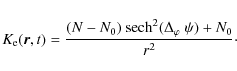
N0 sets the minimum particle density in the magnetized and cold plasma, i.e. between the current sheets, whereas N defines the highest density inside the sheets. However, in order to allow different peak intensity in the light curves, we choose different maximum densities in two consecutive sheets, N1 and N2. This discrepancy could be explained by a different pair creation rate in the two polar caps, feeding the stripes with different numbers of particles. The radial motion of the wind at a fixed speed imposes an overall 1/r2 dependence on this quantity, due to the conservation of the number of particles. An example of particle density number multiplied by this r2 factor for the Geminga pulsar is shown in Fig. 2. Note, however, that adiabatic losses in the current sheets due to pressure work will cool down this distribution function in such a way that
![\begin{figure}
\par\includegraphics[width=8cm,clip]{11010f2.eps}
\end{figure}](/articles/aa/full_html/2009/31/aa11010-08/img41.png) |
Figure 2: The radial variation of the particle density number in the cold magnetized part (low density) and in the current sheets (high density) in the equatorial plane for a given time. The scaling with the factor r2 shows a constant density profile and a slightly different peak intensity in the current sheets. Distances are normalized to the radius of the light cylinder. |
| Open with DEXTER | |
2.3 Inverse Compton emissivity
Let us first recall the general expression for inverse Compton radiation of an electron embedded in an isotropic photon field. We assume an isotropic distribution of mono-energetic target
photons
![]() with density
with density
![]() in the observer frame. The number of photons of energy
in the observer frame. The number of photons of energy
![]() scattered per unit time and per unit frequency by an
ultra-relativistic electron is
scattered per unit time and per unit frequency by an
ultra-relativistic electron is
For convenience, energies of photons are scaled to the rest mass energy of an electron
The power spectrum density of inverse Compton emission is therefore
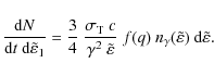
Summing the contribution from each lepton in the distribution function Eq. (7), the total emissivity in the observer frame will be
In the case of ultra-relativistic electrons, their rest mass energy is negligible compared to their kinetic energy and thus they can be treated as massless particles. Their energy (or equivalently their Lorentz factor) then transforms according to the Doppler shift formula for photons
 |
(13) |
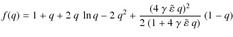
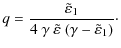
with
![$\displaystyle 2 ~ x^{(p+1)/2} ~
\left[ \frac{1}{p+1}\! -\! \frac{2~x^2}{p+5} \!+\! \frac{2~x~\ln x}{p+3}
\!+\! \frac{p-1}{(p+3)^2} ~ x \right].$](/articles/aa/full_html/2009/31/aa11010-08/img64.png)
The emissivity can therefore be written as
where the upper and lower limits are respectively
Comparing the power index of the Doppler factor in Eq. (3) of Pétri & Kirk (2005) and Eq. (17), the dependence on p is different:
2.4 Light curves and spectra
Knowing the inverse Compton emissivity, the light curves are obtained by integration over the whole wind region. This wind is assumed to extend from a radius r0 to an outer radius
![]() which can be interpreted as the location of the termination shock. However, because of the fast decrease of particle density with radius, there is no need to go so far in practice when performing the numerical integration. Moreover, the radius r0 is interpreted as the transition region between the closed magnetosphere and the launch of the wind. We adopt a sharp unrealistic transition by switching on the emission when crossing this surface. However, in reality we would
expect emission also below this radius. But this region is poorly understood, so we start with this crude model. The shape of the pulses will not be affected by this approximation; it is equivalent to
neglecting some contribution from the DC component. Therefore, the inverse Compton radiation at a fixed observer time t is given by
which can be interpreted as the location of the termination shock. However, because of the fast decrease of particle density with radius, there is no need to go so far in practice when performing the numerical integration. Moreover, the radius r0 is interpreted as the transition region between the closed magnetosphere and the launch of the wind. We adopt a sharp unrealistic transition by switching on the emission when crossing this surface. However, in reality we would
expect emission also below this radius. But this region is poorly understood, so we start with this crude model. The shape of the pulses will not be affected by this approximation; it is equivalent to
neglecting some contribution from the DC component. Therefore, the inverse Compton radiation at a fixed observer time t is given by
The retarded time is expressed as
Table 1: Properties of the Geminga pulsar assuming R*=10 km. Period, distance and magnetic field strength are taken from Taylor et al. (1993).
3 Application to
 -ray pulsars
We apply the aforementioned model to inverse Compton scattering of low-energy photons from the cosmic microwave background with a typical energy of
![]()
![]() 10-4 eV and energy density of 2.65
10-4 eV and energy density of 2.65 ![]()
![]() .
These photons are upscattered from the ultrarelativistic leptons flowing in the current sheets of the striped
wind. The CMB radiation field is assumed to be isotropic. We focus on the Geminga pulsar, for which the useful parameters are listed in Table 1.
.
These photons are upscattered from the ultrarelativistic leptons flowing in the current sheets of the striped
wind. The CMB radiation field is assumed to be isotropic. We focus on the Geminga pulsar, for which the useful parameters are listed in Table 1.
An important parameter of our model is the maximal Lorentz factor reached by pairs. Indeed, it directly determines the cut-off energy in the pulsed spectra. Note also that the minimal Lorentz factor does not play a significant role in fiting the observations. We can find an order of magnitude of
![]() in the following manner. Assuming that the highest energy emanates from the inverse Compton scattering with the CMB, we can deduce the maximal Lorentz factor of
the electrons in the observer frame. Indeed, no pulsed emission is seen above roughly 30 GeV (Thompson 2004). The cut-off energy
in the following manner. Assuming that the highest energy emanates from the inverse Compton scattering with the CMB, we can deduce the maximal Lorentz factor of
the electrons in the observer frame. Indeed, no pulsed emission is seen above roughly 30 GeV (Thompson 2004). The cut-off energy
![]() can be fixed at about 3 GeV. The maximum electron Lorentz factor is therefore obtained by
can be fixed at about 3 GeV. The maximum electron Lorentz factor is therefore obtained by
Thus a typical value is
| |
Figure 3: Gamma-ray light curve above 100 MeV of Geminga fitted with the inverse Compton emission from the striped wind. |
| Open with DEXTER | |
In our best fit, we choose an inclination of the magnetic moment with respect to the rotation axis of
![]() .
In order to obtain a phase separation of 0.5 between the two pulses, we have to adopt an inclination of the line of sight
.
In order to obtain a phase separation of 0.5 between the two pulses, we have to adopt an inclination of the line of sight
![]() .
The Lorentz factor of the wind is
.
The Lorentz factor of the wind is ![]() .
.
Results for the light-curve above 100 MeV and the definition of the different phase intervals are shown in Fig. 3. The rising and falling shape of both pulses are well fitted by our model. In one wavelength of the striped wind, or equivalently in one period of the pulsar, there are two current sheets which give rise to strong emission because of the high density in it. This explains the double pulse structure which is observed at any frequency. Moreover, the two pulses are very similar in shape, with only a difference in maximum intensity. We explain this discrepancy by having slightly different particle density numbers within the current sheets. The corresponding phase-resolved spectra are shown in Fig. 4. The spectral variability is reproduced with satisfactory accuracy except for the OP phase for which the intensity is overestimated.
The intensity and the width of both peaks is matched with good accuracy. Recall that the width is strongly influenced by the size of the current sheets and the Lorentz factor of the wind, due to relativistic beaming effects. For P1, the fitted spectrum lies within the error bars of the EGRET data whereas for P2, the slope is slightly overestimated. Nevertheless, the shape of the cut-off in both cases is retrieved. An excellent fit is also found for the trailing wing 1 (TW1) and the leading wing 2 (LW2). The bridge (BD) and the trailing wing 2 (TW2) follow the same trend. The cut-off although apparent in some phase intervals does not clearly show up in the off-pulse (OP) or in the leading wing 1 (LW1) interval. Observations form the future GLAST satellite will give useful information in this energy band and help to discriminate between different pulsar emission models.
![\begin{figure}
\par\includegraphics[width=8.5cm,clip]{11010f4.eps}
\end{figure}](/articles/aa/full_html/2009/31/aa11010-08/img95.png) |
Figure 4: Phase-resolved inverse Compton emission from the Geminga pulsar for different phase intervals: bridge (BD), leading wing 1/2 (LW1/LW2), off-pulse (OP), peak 1/2 (P1/P2), trailing wing 1/2 (TW1/TW2). The exact definition of these intervals and data are taken from Fierro et al. (1998). |
| Open with DEXTER | |
4 Conclusion
In the striped wind model, the pulsed high-energy emission from pulsars arises from regions well outside the light-cylinder. The geometry of the wind does not depend on the precise magnetospheric structure close to the neutron star surface. Therefore, a detailed model of the physics in the inner pulsar magnetosphere is not required to make robust predictions concerning radiation emanating from the striped wind. By computing the inverse Compton emission on the CMB photons in the Thomson regime, we were able to fit the EGRET data of the light-curves as well as the phase-resolved spectra for at least one gamma-ray pulsar, like Geminga.
Measuring the polarization properties of this high-energy emission would provide a valuable diagnostic of the physical process responsible for these MeV-GeV photons. In the future, experiments are planned to measure the polarization in X-rays or gamma-rays, like the PoGOLite satellite (Kamae et al. 2007).
Because the radiation is mostly emanating from the base of the striped wind where the density of particles is highest, a better description of the transition between the closed magnetosphere and the wind is required to obtain a detailed view of the magnetic field configuration.
Note also that the same kind of computation can be performed for the Crab pulsar, for which we know the polarization properties in optical bands and can therefore predict the polarization at higher energies by extrapolation.
Acknowledgements
I am grateful to John Kirk for helpful discussions and suggestions and to Dave Thompson for sending me the EGRET data. This work was partly supported by a grant from the G.I.F., the German-Israeli Foundation for Scientific Research and Development.
References
- Arons, J. 1979, Space Sci. Rev., 24, 437 [NASA ADS] [CrossRef] (In the text)
- Blumenthal, G. R., & Gould, R. J. 1970, Rev. Mod. Phys., 42, 237 [NASA ADS] [CrossRef] (In the text)
- Bogovalov, S. V. 1999, A&A, 349, 1017 [NASA ADS]
- Bogovalov, S. V., & Aharonian, F. A. 2000, MNRAS, 313, 504 [NASA ADS] [CrossRef] (In the text)
- Cheng, K. S., Ho, C., & Ruderman, M. 1986, ApJ, 300, 500 [NASA ADS] [CrossRef] (In the text)
- Coroniti, F. V. 1990, ApJ, 349, 538 [NASA ADS] [CrossRef] (In the text)
- Daugherty, J. K., & Harding, A. K. 1996, ApJ, 458, 278 [NASA ADS] [CrossRef] (In the text)
- Dokuchaev, V. P., Ramoikin, V. V., & Chugunov, Y. V. 1976, SvA, 20, 299 [NASA ADS] (In the text)
- Ferrari, A., & Trussoni, E. 1975, Ap&SS, 33, 111 [NASA ADS] [CrossRef]
- Fierro, J. M., Michelson, P. F., Nolan, P. L., & Thompson, D. J. 1998, ApJ, 494, 734 [NASA ADS] [CrossRef] (In the text)
- Georganopoulos, M., Kirk, J. G., & Mastichiadis, A. 2001, ApJ, 561, 111 [NASA ADS] [CrossRef] (In the text)
- Grewing, M., & Heintzmann, H. 1971, Astrophys. Lett., 8, 167 [NASA ADS] (In the text)
- Kamae, T., Andersson, V., Arimoto, M., et al. 2007, arXiv e-prints, 709 (In the text)
- Kirk, J. G. 1994, in Saas-Fee Advanced Course 24: Plasma Astrophysics, ed. A. O. Benz, & T. J.-L. Courvoisier, 225 (In the text)
- Kirk, J. G., Skjæraasen, O., & Gallant, Y. A. 2002, A&A, 388, L29 [NASA ADS] [CrossRef] [EDP Sciences]
- Lerche, I. 1970a, ApJ, 159, 229 [NASA ADS] [CrossRef] (In the text)
- Lerche, I. 1970b, ApJ, 160, 1003 [NASA ADS] [CrossRef]
- Lerche, I. 1970c, ApJ, 162, 153 [NASA ADS] [CrossRef]
- Lyubarskii, Y. E. 1996, A&A, 311, 172 [NASA ADS]
- Michel, F. C. 1971, Comm. Astrophys. Space Phys., 3, 80 [NASA ADS] (In the text)
- Michel, F. C. 1994, ApJ, 431, 397 [NASA ADS] [CrossRef] (In the text)
- Michel, F. C., & Tucker, W. H. 1969, Nature, 223, 277 [NASA ADS] [CrossRef] (In the text)
- Pétri, J., & Kirk, J. G. 2005, ApJ, 627, L37 [NASA ADS] [CrossRef] (In the text)
- Pétri, J., & Kirk, J. G. 2007, Plasma Physics and Controlled Fusion, 49, 1885 [NASA ADS] [CrossRef] (In the text)
- Romani, R. W. 1996, ApJ, 470, 469 [NASA ADS] [CrossRef] (In the text)
- Ruderman, M. A., & Sutherland, P. G. 1975, ApJ, 196, 51 [NASA ADS] [CrossRef] (In the text)
- Tademaru, E. 1971, Ap&SS, 12, 193 [NASA ADS] [CrossRef]
- Taylor, J. H., Manchester, R. N., & Lyne, A. G. 1993, ApJS, 88, 529 [NASA ADS] [CrossRef] (In the text)
- The MAGIC Collaboration, Aliu, E., et al. 2008, ArXiv e-prints, 809 (In the text)
- Thompson, D. J. 2003, arXiv Astrophysics e-prints (In the text)
- Thompson, D. J. 2004, in IAU Symp., ed. F. Camilo, & B. M. Gaensler, 399 (In the text)
- Thompson, D. J. 2007, arXiv e-prints, 711 (In the text)
- Zhang, L., & Cheng, K. S. 2001, MNRAS, 320, 477 [NASA ADS] [CrossRef] (In the text)
All Tables
Table 1: Properties of the Geminga pulsar assuming R*=10 km. Period, distance and magnetic field strength are taken from Taylor et al. (1993).
All Figures
| |
Figure 1: Structure of the azimuthal magnetic field in the equatorial plane at a given time. Note the smooth polarity reversal when crossing the current sheets. The scaling by a factor r removes the radial decrease of the amplitude and helps to better visualize the thickness of the current sheets. Distances are normalized to the radius of the light cylinder. |
| Open with DEXTER | |
| In the text | |
| |
Figure 2: The radial variation of the particle density number in the cold magnetized part (low density) and in the current sheets (high density) in the equatorial plane for a given time. The scaling with the factor r2 shows a constant density profile and a slightly different peak intensity in the current sheets. Distances are normalized to the radius of the light cylinder. |
| Open with DEXTER | |
| In the text | |
| |
Figure 3: Gamma-ray light curve above 100 MeV of Geminga fitted with the inverse Compton emission from the striped wind. |
| Open with DEXTER | |
| In the text | |
| |
Figure 4: Phase-resolved inverse Compton emission from the Geminga pulsar for different phase intervals: bridge (BD), leading wing 1/2 (LW1/LW2), off-pulse (OP), peak 1/2 (P1/P2), trailing wing 1/2 (TW1/TW2). The exact definition of these intervals and data are taken from Fierro et al. (1998). |
| Open with DEXTER | |
| In the text | |
Copyright ESO 2009
Current usage metrics show cumulative count of Article Views (full-text article views including HTML views, PDF and ePub downloads, according to the available data) and Abstracts Views on Vision4Press platform.
Data correspond to usage on the plateform after 2015. The current usage metrics is available 48-96 hours after online publication and is updated daily on week days.
Initial download of the metrics may take a while.