| Issue |
A&A
Volume 502, Number 3, August II 2009
|
|
|---|---|---|
| Page(s) | 833 - 844 | |
| Section | Interstellar and circumstellar matter | |
| DOI | https://doi.org/10.1051/0004-6361/200811549 | |
| Published online | 15 June 2009 | |
Predictions of polarized dust emission from interstellar clouds: spatial variations in the efficiency of radiative torque alignment
V.-M. Pelkonen1 - M. Juvela1 - P. Padoan2
1 - Observatory, University of Helsinki, Tähtitorninmäki, PO Box 14, 00014 University of Helsinki, Finland
2 -
Department of Physics, University of California, San Diego, CASS/UCSD 0424, 9500 Gilman Drive, La Jolla, CA 92093-0424, USA
Received 19 December 2008 / Accepted 29 April 2009
Abstract
Context. Polarization carries information about the magnetic fields in interstellar clouds. The observations of polarized dust emission are used to study the role of magnetic fields in the evolution of molecular clouds and the initial phases of star formation. Therefore, it is important to understand how different cloud regions contribute to the observed polarized signal.
Aims. We study the grain alignment with realistic simulations, assuming the radiative torques to be the main mechanism. The aim is to study the efficiency of the grain alignment as a function of cloud position and to study the observable consequences of these spatial variations.
Methods. Our results are based on the analysis of model clouds derived from MHD simulations of super-Alfvénic magnetized turbulent flows. The continuum radiative transfer problem is solved with Monte Carlo methods to estimate the three-dimensional distribution of dust emission and the radiation field strength. The anisotropy of the radiation field is taken into account explicitly. We also examine the effect of grain growth in cores both to the observed polarization and to the inferred magnetic field.
Results. Using the assumptions of Cho & Lazarian (2005, ApJ, 631, 361), our findings are generally consistent with their results. However, the anisotropy factor is lower than their assumption of
![]() ,
and thus radiative torques are less efficient. Compared with our previous paper, P/I relations are steeper. Without grain growth, the magnetic field of the cores is poorly recovered above a few
,
and thus radiative torques are less efficient. Compared with our previous paper, P/I relations are steeper. Without grain growth, the magnetic field of the cores is poorly recovered above a few ![]() .
If grain size is doubled, the polarized dust emission can trace the magnetic field lines possibly up to
.
If grain size is doubled, the polarized dust emission can trace the magnetic field lines possibly up to
![]() mag. However, many of the prestellar cores may be too young for grain coagulation to play a major role. The inclusion of direction-dependent radiative torque efficiency weakens the alignment. Even with doubled grain size, we would not expect to probe the magnetic field beyond a few magnitudes in
mag. However, many of the prestellar cores may be too young for grain coagulation to play a major role. The inclusion of direction-dependent radiative torque efficiency weakens the alignment. Even with doubled grain size, we would not expect to probe the magnetic field beyond a few magnitudes in ![]() .
.
Key words: ISM: dust, extinction - ISM: clouds - polarization - radiative transfer
1 Introduction
Magnetic fields are important in many astrophysical processes. In star formation, the magnetic pressure may support an otherwise gravitationally unstable cloud core against collapse. Magnetohydrodynamical models allow predictions of what magnetic fields might look like in interstellar clouds and protostellar cores, but the models need to be tested against observations. Information about interstellar magnetic fields can be derived with different techniques. Amongst the most useful are the polarization of starlight from background stars and the polarized thermal dust emission at longer wavelengths, which arise from the alignment of the spin axis of the dust grains along the magnetic field.
The main question with dust polarization is the alignment mechanism, or
rather, what makes the dust grains spin up in the first place? One of the
earliest mechanisms proposed was the paramagnetic mechanism (Davis &
Greenstein 1951), which is based on the direct interaction of
rotating grains with the interstellar magnetic field. However, to explain the
grain alignment needed for the polarization, this mechanism
requires much stronger magnetic fields than have been observed. Purcell (1979)
introduced several processes that could cause the grains to become very fast rotators,
and suggested that ![]() -ejection might be a major cause of fast grain
rotation. However, further investigations of
-ejection might be a major cause of fast grain
rotation. However, further investigations of ![]() -ejection identified
several related processes that make it inefficient in aligning dust
grains, such as grain wobbling (e.g., Jones & Spitzer 1967; Lazarian
1994; Lazarian & Roberge 1997), grain flipping (Lazarian &
Draine 1999a), and ``nuclear relaxation'' (Lazarian & Draine
1999b). These mechanisms and others were discussed in a review
paper by Lazarian (2007).
-ejection identified
several related processes that make it inefficient in aligning dust
grains, such as grain wobbling (e.g., Jones & Spitzer 1967; Lazarian
1994; Lazarian & Roberge 1997), grain flipping (Lazarian &
Draine 1999a), and ``nuclear relaxation'' (Lazarian & Draine
1999b). These mechanisms and others were discussed in a review
paper by Lazarian (2007).
The radiative torque mechanism has become a strong candidate for the primary mechanism of grain alignment inside molecular clouds. The radiative torque mechanism involves the transfer of momentum by collisions of photons onto the grain, causing a torque that rotates the grain around its axis. It was first introduced by Dolginov (1972) and Dolginov & Mytrophanov (1976). The efficiency of the radiative torques has been demonstrated using numerical simulations (Draine & Weingartner 1996, 1997) and in a laboratory setup (Abbas et al. 2004). The predictions of the radiative torque mechanisms are roughly consistent with observations (e.g., Lazarian et al. 1997; Hildebrand et al. 2000).
However, Draine & Weingartner (1996) were incorrect to assume that the grains would just be spun up by radiative torques, and aligned by paramagnetic relaxation. In their subsequent paper, Draine & Weingartner (1997) confirmed that radiative torques would be able to align grains on their own, without relying on paramagnetic relaxation. Lazarian & Draine (1999a) showed that thermal flipping would prevent the paramagnetic alignment mechanism being effective in small grains.
Cho & Lazarian (2005) used a spherically symmetric model cloud
to calculate the size of grains aligned by radiative torques, assuming a
constant anisotropy factor,
![]() ,
and neglecting the isotropic
component of the radiation. Their calculations showed that even deep inside
GMCs (
,
and neglecting the isotropic
component of the radiation. Their calculations showed that even deep inside
GMCs (
![]() ), large grains can still be aligned by radiative torques.
Cho & Lazarian (2005) presented an empirical formula for the
minimum size of the aligned grain
), large grains can still be aligned by radiative torques.
Cho & Lazarian (2005) presented an empirical formula for the
minimum size of the aligned grain
![]() as a function of the density
as a function of the density ![]() and extinction
and extinction ![]() ,
which is
,
which is
The formula is, strictly speaking, only valid for spherically symmetric clouds, and carries the additional assumption of a constant anisotropy factor,
The obvious next step is to complete radiative transfer calculations in more detail, derive the actual anisotropy within an inhomogeneous cloud, and use it to
calculate the efficiency of radiative torques. Similar work was carried out by Bethell et al. (2007). These authors were able to derive P/I relations reminiscent of the observed ones, and their results agreed with the qualitative results of Cho & Lazarian (2005). They found that simplifying assumptions about the radiative anisotropy (e.g., a constant value of ![]() )
have only a moderate effect on the emergent degree of polarization.
)
have only a moderate effect on the emergent degree of polarization.
In the present paper, we study the anisotropy factor ![]() and calculate the minimum sizes of the
aligned grains within our model clouds. In addition to calculating 1D models
to compare with Eq. (1), we also compare our results with those of our previous 3D
models (Pelkonen et al. 2007). We investigate quantitatively
the effects that grain growth has on the polarized signal expected from dense
cloud cores. In particular, we examine a model where the grain growth is restricted to the densest regions. Furthermore, we examine where the observed polarization actually originates along the line of sight.
and calculate the minimum sizes of the
aligned grains within our model clouds. In addition to calculating 1D models
to compare with Eq. (1), we also compare our results with those of our previous 3D
models (Pelkonen et al. 2007). We investigate quantitatively
the effects that grain growth has on the polarized signal expected from dense
cloud cores. In particular, we examine a model where the grain growth is restricted to the densest regions. Furthermore, we examine where the observed polarization actually originates along the line of sight.
In the past few years, our understanding of the radiative torques has been improving rapidly. Lazarian & Hoang (2007) presented the first analytic model of radiative torques, allowing for quantitative treatment of radiative torque alignment. At the time of submission of this paper, Hoang & Lazarian (2008b) expanded their treatment of radiative torques from beam radiation fields to dipole and quadrupole fields, and illustrated the dependence of radiative torque efficiency on the angle between the magnetic field and the radiation. These important steps should be included in future studies of polarization within clumpy clouds. In this paper, we present an example where we take into account the angle between the local magnetic field and the direction of the anisotropic beam radiation to quantify the effect that it will have on emergent polarization.
2 The basic equations
To calculate the alignment efficiency of radiative torques, we follow the formalism presented in Draine & Weingartner (1996). The rotational
damping time due to gas drag is
| |
= | ||
 |
(2) |
where
where
and
If we assume that the grain is illuminated by an isotropic radiation component
![]() and an anisotropic radiation component
and an anisotropic radiation component
![]() ,
a steady
radiative torque gives the grain an angular velocity (Eq. (65) in Draine & Weingartner 1996)
,
a steady
radiative torque gives the grain an angular velocity (Eq. (65) in Draine & Weingartner 1996)
where
The randomization of the rotation of the grain is caused by
collisions with gas molecules. When the grain rotates much more rapidly than the thermal rotation rate,
this randomization is greatly reduced. Thus, a suprathermally rotating grain is expected to be aligned with the magnetic field. The factor between the rotational rate due to the radiative torques,

3 Polarization
3.1 Rayleigh polarization reduction factor
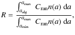
The Rayleigh polarization reduction factor R is a measure of the imperfect
alignment of dust grains with respect to the magnetic field (Greenberg
1968; see also Lee & Draine 1985). The degree of
polarization is reduced when grains are not aligned with the magnetic
field. In the case of radiative torques, smaller grains are not aligned but
larger grains are. The minimum aligned grain size,
![]() ,
is
derived from Eq. (7), such that
,
is
derived from Eq. (7), such that
![]() when
when
![]() .
.
The polarization reduction factor is
where
![\begin{figure}
\par\includegraphics[width=8cm,clip]{11549_01.eps}
\end{figure}](/articles/aa/full_html/2009/30/aa11549-08/img57.png) |
Figure 1:
Polarization reduction factor R as a function of
|
| Open with DEXTER | |
3.2 Polarized thermal dust emission
The polarized thermal dust emission is calculated following the formalism in Fiege & Pudritz (2000). Self-absorption and scattering can be neglected at submillimeter wavelengths. The Stokes Q and U components are equal to the integrals
where
The polarization angle ![]() is given by
is given by
| (11) |
and the degree of polarization P is

with
| (13) |
and
| (14) |
where
The coefficient ![]() is defined as
is defined as

where R is the Rayleigh polarization reduction factor due to imperfect grain alignment, F is the polarization factor due to the turbulent component of the magnetic field,
In our study, F = 1 because the three-dimensional magnetic field is given by
the MHD models, and we assume that the small-scale structure is resolved in
the numerical solution. The ratio
![]() needs to be fixed
because we want to study the effects caused by variations in R. To avoid
an unreasonably high polarization degree, we choose
needs to be fixed
because we want to study the effects caused by variations in R. To avoid
an unreasonably high polarization degree, we choose
![]() .
This corresponds to the axial ratio of roughly 1.1 (see Fig. 1 in
Padoan et al. 2001).
.
This corresponds to the axial ratio of roughly 1.1 (see Fig. 1 in
Padoan et al. 2001).
4 Radiative transfer calculations
To calculate the amount of polarized dust emission, we needed to carry out radiative transfer modeling, to (1) calculate the intensity and angular distribution of the radiation field, (2) determine the resulting total intensity of dust emission, and (3) determine the dust temperature. Apart from determining the total emission, dust temperatures affect thermal rotation rates and, thereby, the minimum size of aligned grains. The intensity of the incoming radiation and its anisotropy affect the magnitude of the rotational torques, as shown in Eq. (7).
The radiative transfer calculations are made with a Monte Carlo program
(Juvela & Padoan 2003), where the contribution of transiently heated,
small grains is also solved. To determine the anisotropy of the
radiation field within the model clouds, the photons entering each
computational cell were registered. The angular distribution was tracked by
binning the photons into 12 bins that corresponded to angular discretization
according to the Healpix scheme (Gorski et al. 2005). The anisotropy of the radiation field
was estimated by calculating the vector sum of the intensity over different
directions. We made the simplifying assumption that the radiative torque
efficiency is direction invariant and that opposing directions cancel out. The
remaining part was our anisotropic radiation component. When the anisotropic
component was subtracted from the total radiation, we were left with the
isotropic component. Based on Table 4 in Draine & Weingartner (1996), we assumed that
![]() ,
where
,
where
![]() is the radiative torque efficiency for anisotropic radiation, shown in Fig. 2. We used the dust model discussed in Li & Draine (2001).
is the radiative torque efficiency for anisotropic radiation, shown in Fig. 2. We used the dust model discussed in Li & Draine (2001).
![\begin{figure}
\par\includegraphics[width=8cm,clip]{11549_02.eps}
\end{figure}](/articles/aa/full_html/2009/30/aa11549-08/img76.png) |
Figure 2:
Radiative torque efficiency
|
| Open with DEXTER | |
Finally, we calculated an example where we took the direction dependence of the radiative torque efficiency from Fig. 17 in Hoang & Lazarian (2008b). We normalized the unidirectional curve to 1 when the radiation vector and the magnetic field vector are parallel, and used the resulting curve as our direction-dependent efficiency factor. The efficiency factor drops by more than a factor of ten when moving towards a perpendicular orientation of the vectors. We considered neither multipoles nor isotropy in this simplified example, but multiplied each beam direction by the efficiency factor, and calculated the vector sum of our anisotropy. This anisotropic radiation intensity was then used to calculate the aligned grain size.
5 The model clouds
We examine briefly one spherically symmetric cloud model for which the
density distribution is obtained from the Bonnor-Ebert solution of hydrostatic
equilibrium (Bonnor 1956; Ebert 1955). The mass of the cloud is 3.7
![]() and, for a stability parameter value of
and, for a stability parameter value of ![]() ,
the visual extinction to the cloud center is
,
the visual extinction to the cloud center is
![]() .
When the
total opacity of the cloud is fixed the exact value of the parameter
.
When the
total opacity of the cloud is fixed the exact value of the parameter ![]() is
not important. For a given distance from the cloud surface, measured in
is
not important. For a given distance from the cloud surface, measured in
![]() ,
the local intensity and anisotropy of the radiation field
depend only weakly on the true shape of the density profile.
,
the local intensity and anisotropy of the radiation field
depend only weakly on the true shape of the density profile.
Our main interest lies in the study of inhomogeneous, three-dimensional clouds. We revisit the model C discussed by Pelkonen et al. (2007). It is based on the results of numerical simulations of highly supersonic magnetohydrodynamic turbulence, completed for a 1283 computational mesh with periodic boundary conditions (for details, see Pelkonen et al. 2007).
![\begin{figure}
\par\includegraphics[width=16cm,clip]{11549_03.eps}
\end{figure}](/articles/aa/full_html/2009/30/aa11549-08/img81.png) |
Figure 3:
|
| Open with DEXTER | |
In addition, we study three cloud cores that are taken from a new simulation of
supersonic and super-Alfvénic MHD simulation. The MHD simulation was run on
a mesh of 10003 computational cells with the Stagger Code (Padoan et al.
2007), re-meshed to 10243. In the used snapshot the rms sonic Mach number is 8.9
and the rms Alfvénic Mach number is 2.8, so that the turbulence is still
super-Alfvénic even with respect to the rms Alfvén velocity. From the
10243 volume, we selected three dense regions (``clumps''), each 1283cells in size (see Fig. 3). The average density
of the 10243 cloud was scaled to
![]() cm-3 and its linear
size was set to be 6 pc. This corresponds to an average visual extinction of
cm-3 and its linear
size was set to be 6 pc. This corresponds to an average visual extinction of
![]() 3
3![]() .
In the selected core regions the visual extinction is higher,
reaching peak values of 10.9, 23.7, and 21.8 mag in the three cores,
respectively. The radiative transfer is solved locally for the subgrids of 1283 grid points rather than the full 10243 mesh.
.
In the selected core regions the visual extinction is higher,
reaching peak values of 10.9, 23.7, and 21.8 mag in the three cores,
respectively. The radiative transfer is solved locally for the subgrids of 1283 grid points rather than the full 10243 mesh.
6 Results
6.1 Spherically symmetric cloud
We start by looking at grain alignment in the case of the spherically
symmetric cloud described in Sect. 5. Figure 4 shows the anisotropy factors at different wavelengths. The intensity of the short wavelength radiation drops sharply with ![]() ,
but the anisotropy increases since the remaining intensity comes preferentially from smaller and smaller space angles. At longer wavelengths, the dust emission starts to dominate over ISRF and the direction of the anisotropy is towards the surface, although the effect on effective
,
but the anisotropy increases since the remaining intensity comes preferentially from smaller and smaller space angles. At longer wavelengths, the dust emission starts to dominate over ISRF and the direction of the anisotropy is towards the surface, although the effect on effective ![]() is small. At the center of the spherically symmetric cloud the anisotropy is by definition zero.
is small. At the center of the spherically symmetric cloud the anisotropy is by definition zero.
Figure 5 shows the comparison of Eq. (1) and our results with constant
![]() and
and ![]() calculated from the radiative transfer calculations. The number of grains larger than 0.58
calculated from the radiative transfer calculations. The number of grains larger than 0.58
![]() in Li & Draine (2001) dust model is negligible. Thus, Fig. 5 shows that according to this calculation, there is essentially no alignment above 3 mag, while in the Cho & Lazarian model the limit is 5 mag. Larger grains, if they exist, could be aligned by radiative torques at higher
in Li & Draine (2001) dust model is negligible. Thus, Fig. 5 shows that according to this calculation, there is essentially no alignment above 3 mag, while in the Cho & Lazarian model the limit is 5 mag. Larger grains, if they exist, could be aligned by radiative torques at higher ![]() .
In an inhomogeneous cloud there might also be some sightlines of lower
.
In an inhomogeneous cloud there might also be some sightlines of lower ![]() ,
which produce more efficient radiative torques.
,
which produce more efficient radiative torques.
6.2 Three-dimensional MHD models
The dust polarization was studied in three-dimensional models described in Sect. 5. Figure 6 shows the calculated polarization maps at 353 GHz for our old 3D model C, used in Pelkonen et al. (2007). The polarization degree has been reduced everywhere, as expected from Fig. 5, but particularly in high density regions. This reduction in the polarization degree is more readily apparent in Fig. 7, where the P/I slopes of most of the selected cores are steeper with the new calculations. This is because in a clumpy medium, starlight can penetrate the cloud from many different directions rather than in a clearly defined ``brightest'' direction. Thus, the anisotropy will be averaged out somewhat, leading to weaker radiative torques and lower polarized emission. In the cores themselves the anisotropy is even less, so the difference with an invariant
![]() is greater, resulting in a steeper slope.
is greater, resulting in a steeper slope.
![\begin{figure}
\par\includegraphics[width=8.9cm,clip]{11549_04.eps}
\end{figure}](/articles/aa/full_html/2009/30/aa11549-08/img86.png) |
Figure 4: The anisotropy factors at different wavelengths inside a 1D model cloud. The thick lines are without and the thin lines with dust emission. |
| Open with DEXTER | |
![\begin{figure}
\par\includegraphics[width=8.5cm,clip]{11549_05.eps}
\end{figure}](/articles/aa/full_html/2009/30/aa11549-08/img87.png) |
Figure 5: Comparison of Eq. (1) ( dashed) and our results ( solid, dotted) for the Bonnor-Ebert sphere model. |
| Open with DEXTER | |
Figures 8 and 9 show similar plots for our new high resolution model at 353 GHz. In Fig. 8, the vectors are drawn for polarized intensity, not for polarization degree, which is why long vectors are superimposed on the bright, high density regions. In Fig. 9, Core 1, when viewed from the z direction, does not seem to show a clear decrease in the polarization degree, unlike the other examples. This is because Core 1 is less dense, and the maximum visual extinction through the core in the z direction is only 3.9 mag. This also explains why the other two relations for Core 1 are not as steep as for Cores 2 and 3, because radiation can penetrate the core much more easily.
In dense clumps, grain coagulation can cause the grains to grow, shifting the size distribution to larger grain sizes. We took Core 2 and multiplied the density by ten to obtain a dense cloud. Figure 10 shows the anisotropy in a slice in the mid-plane, as well as density contours. In Fig. 11, we show the polarization degree for three different dust size distributions for this high density model. We first calculated the grain alignment and dust emission using normal Li & Draine (2001) dust. The polarization degree is rather low and declines over the complete intensity interval. Secondly, we calculated the alignment by assuming that all our dust grains were double their original size. The shape of the radiative field inside the cloud should be closely the same, and we were only interested in the polarization degree and scaled intensity rather than absolute values of intensity. Thus, we used the same
![]() as for normal dust and simply used the doubled grain size distribution shown by Eq. (8), resulting in more efficient polarization.
as for normal dust and simply used the doubled grain size distribution shown by Eq. (8), resulting in more efficient polarization.
![\begin{figure}
\par\includegraphics[width=15.85cm,clip]{11549_06.eps}
\end{figure}](/articles/aa/full_html/2009/30/aa11549-08/img88.png) |
Figure 6: Simulated polarization maps at 353 GHz with R calculated using Eq. (1) ( left frame) and Eq. (7). Polarization vectors are drawn for every third pixel and the scaling of the vector lengths is the same in both frames, representing the polarization degree. In the left frame the maximum polarization degree is 8.5%, while in the right frame it is 7.3%. The background image shows the logarithm of the total intensity at this frequency. |
| Open with DEXTER | |
![\begin{figure}
\par\includegraphics[width=16cm,clip]{11549_07.eps}
\end{figure}](/articles/aa/full_html/2009/30/aa11549-08/img89.png) |
Figure 7:
The relation between polarization degree and total intensity for selected cores of the polarization maps in Fig. 6. Cyan dots show the old results (Eq. (1)), assuming constant |
| Open with DEXTER | |
![\begin{figure}
\par\includegraphics[width=15cm,clip]{11549_08.eps}
\end{figure}](/articles/aa/full_html/2009/30/aa11549-08/img90.png) |
Figure 8: Simulated polarization maps of the high resolution model at 353 GHz. Polarization vectors are drawn for every fifth pixel, the length corresponding to the polarized intensity. The background image shows the logarithm of the total intensity. The scaling of the background and the length of the vectors are the same in all frames, the longest vector being 0.11 MJy/sr. |
| Open with DEXTER | |
where
![\begin{figure}
\par\includegraphics[width=16cm,clip]{11549_09.eps}
\end{figure}](/articles/aa/full_html/2009/30/aa11549-08/img98.png) |
Figure 9: The relation between polarization degree and total intensity for the polarization maps in Fig. 8. In order to avoid cluttering the plot, only every fifth map pixel along both horizontal and vertical direction is plotted. |
| Open with DEXTER | |
Where does the observed polarized emission originate? The thermal dust emission tends to trace the density structure. High density means more emitting dust and thus higher emission, although the temperature is anticorrelated with density and thus complicates the picture. However, Figs. 1 and 5 hint that above a couple of ![]() only a fraction of the grains are aligned, and thus the polarization degree drops sharply. Figure 12 shows the polarized intensity and the gas density in each cell along lines of sight through each of the cores as seen from three different viewing directions. The effect of shadowing by even modest density structures is striking, as is the absence or reduction in the polarized emission from the densest structures. In Core 2, the polarized emission is also plotted for the doubled grain size. In this case, the polarized emission originates deeper inside the core. However, because of the high local density, the density maximums in the y and x directions still do not have aligned grains. The z direction exhibits significant polarized emission from the density maximum even though the visual extinction along that line of sight is greater. In Core 1, the magnetic field is oriented almost towards the observer in the z direction, which is why the polarization is weakened.
only a fraction of the grains are aligned, and thus the polarization degree drops sharply. Figure 12 shows the polarized intensity and the gas density in each cell along lines of sight through each of the cores as seen from three different viewing directions. The effect of shadowing by even modest density structures is striking, as is the absence or reduction in the polarized emission from the densest structures. In Core 2, the polarized emission is also plotted for the doubled grain size. In this case, the polarized emission originates deeper inside the core. However, because of the high local density, the density maximums in the y and x directions still do not have aligned grains. The z direction exhibits significant polarized emission from the density maximum even though the visual extinction along that line of sight is greater. In Core 1, the magnetic field is oriented almost towards the observer in the z direction, which is why the polarization is weakened.
Figure 13 shows the histogram of both the intensity and the fraction of polarized intensity in different density bins for Core 2 seen along the z direction. Due to the summing of the contribution of the individual cells in each bin, we need to compare the total intensity contribution with the polarized emission contribution. The high density cells contribute less and less to the polarized emission, while the contribution of the small density cells is enhanced. With doubled grain sizes, the more efficient grain alignment is clearly evident because the polarized emission still comes from higher density regions, before finally falling, too.
![\begin{figure}
\par\includegraphics[width=8cm]{11549_10.eps}
\end{figure}](/articles/aa/full_html/2009/30/aa11549-08/img101.png) |
Figure 10:
The anisotropy factor
|
| Open with DEXTER | |
![\begin{figure}
\par\includegraphics[width=8cm]{11549_11.eps}
\end{figure}](/articles/aa/full_html/2009/30/aa11549-08/img102.png) |
Figure 11: The relation between polarization degree and total intensity for Core 2 (see Fig. 9) where the density has been multiplied by ten. The figure shows the polarization degree observed towards the z direction. The polarized dust emission is calculated for doubled (approximate calculation, see text) and normal grain sizes, and for a mixed distribution where larger grains are found only in dense regions (see text). |
| Open with DEXTER | |
![\begin{figure}
\par\includegraphics[width=16cm]{11549_12.eps}
\end{figure}](/articles/aa/full_html/2009/30/aa11549-08/img103.png) |
Figure 12:
The gas density,
|
| Open with DEXTER | |
Do polarization vectors trace the magnetic field with any degree of certainty? Above a threshold, which depends on the local density as well as the geometry of the cloud, the radiative torque alignment is no longer capable of organizing the grain orientation. Thus the emission from shielded region is unpolarized, giving the observer no information about the magnetic field within it.
![\begin{figure}
\par\includegraphics[width=8cm]{11549_13.eps}
\end{figure}](/articles/aa/full_html/2009/30/aa11549-08/img104.png) |
Figure 13: A histogram showing the contribution of different density cells to the total intensity ( solid line), and to the polarized intensity for normal grain sizes ( dashed line) and doubled grain sizes ( dotted line). This is for Core 2 and the local polarized emission as seen from the z direction. The total and polarized intensity are shown as sums of all emission from the cells in that bin; thus the few high density cells have a low contribution to total intensity. All intensities are at 353 GHz. |
| Open with DEXTER | |
Figure 14 shows the rms errors between the observed polarization angle,
![]() ,
and the volume- and the mass-averaged magnetic field angles,
,
and the volume- and the mass-averaged magnetic field angles,
![]() and
and
![]() .
For low
.
For low ![]() ,
,
![]() and
and
![]() agree well, because there are no dense clumps along the line of sight where the radiative torque alignment would be inefficient. Temperature differences between warm diffuse regions and cold denser regions do introduce some discrepancies caused by the different weighting in emission and in density. For higher
agree well, because there are no dense clumps along the line of sight where the radiative torque alignment would be inefficient. Temperature differences between warm diffuse regions and cold denser regions do introduce some discrepancies caused by the different weighting in emission and in density. For higher ![]() ,
the situation changes;
,
the situation changes;
![]() traces the magnetic field directions in the dense clumps, while the influence of dense clumps on
traces the magnetic field directions in the dense clumps, while the influence of dense clumps on
![]() is reduced by the weakened radiative torque alignment. This is because the radiative torque alignment continues to be effective on the larger grains, and the dense clumps continue to contribute to the polarized emission. Any emission or density variations are not taken into account by
is reduced by the weakened radiative torque alignment. This is because the radiative torque alignment continues to be effective on the larger grains, and the dense clumps continue to contribute to the polarized emission. Any emission or density variations are not taken into account by
![]() ,
and thus the difference between observed and volume-averaged angles depends greatly on the density profile and the local magnetic field orientation. If the density profile is flat or the magnetic field is ordered apart from the densest clumps, then
,
and thus the difference between observed and volume-averaged angles depends greatly on the density profile and the local magnetic field orientation. If the density profile is flat or the magnetic field is ordered apart from the densest clumps, then
![]() .
.
![\begin{figure}
\par\includegraphics[width=16cm]{11549_14.eps}
\end{figure}](/articles/aa/full_html/2009/30/aa11549-08/img109.png) |
Figure 14: The rms difference between the observed polarization angles and the mass-averaged ( dashed line) and volume-averaged ( dotted line) magnetic field directions, for all cores and viewing directions. The observed polarization angles are calculated with normal Li & Draine (2001) grain size distribution. For Core 2 polarization was also calculated with doubled grain sizes, and compared with mass-averaged ( thick solid line) and volume-averaged ( thick dash-dot line) magnetic field direction. |
| Open with DEXTER | |
At the highest ![]() ,
there are only a few independent structures (see Fig. 12), and the different magnetic field geometries play a crucial role. Taking Core 2 as an example, there is one structure along the z-axis. In that structure, two clumps along the line of sight have their magnetic fields aligned anti-parallel. Their combined signal is mostly unpolarized, and thus
,
there are only a few independent structures (see Fig. 12), and the different magnetic field geometries play a crucial role. Taking Core 2 as an example, there is one structure along the z-axis. In that structure, two clumps along the line of sight have their magnetic fields aligned anti-parallel. Their combined signal is mostly unpolarized, and thus
![]() .
That is why the rms remains flat even to high
.
That is why the rms remains flat even to high ![]() .
The same would happen if both clumps had a magnetic field direction close to
.
The same would happen if both clumps had a magnetic field direction close to
![]() ,
in which case the contribution of the clumps - whether total (
,
in which case the contribution of the clumps - whether total (
![]() )
or partial (
)
or partial (
![]() )
- would only reinforce the orientation from the diffuse regions. Along the y-axis, the density profile is quite varied, as is the magnetic field orientation, and thus none of the angles agree at high
)
- would only reinforce the orientation from the diffuse regions. Along the y-axis, the density profile is quite varied, as is the magnetic field orientation, and thus none of the angles agree at high ![]() .
Finally, along the x-axis, direction of the mass-averaged magnetic field is determined mostly by one high density clump, where the magnetic field direction spins around. Thus,
.
Finally, along the x-axis, direction of the mass-averaged magnetic field is determined mostly by one high density clump, where the magnetic field direction spins around. Thus,
![]() but
but
![]() .
As always with polarization, one cannot ignore the geometrical effects.
.
As always with polarization, one cannot ignore the geometrical effects.
From Fig. 14, it can be seen that an rms difference of 10-30 degrees is common for sightlines of higher extinction than a few ![]() .
This difference arises because the grains are not aligned in the dense regions of the cloud, and thus the dense regions do not contribute to the observed polarization. This may cause problems for the Chandrasekhar-Fermi method (Chandrasekhar & Fermi 1953) and in attempts to infer core formation processes based on the relative alignment of B and core geometry.
.
This difference arises because the grains are not aligned in the dense regions of the cloud, and thus the dense regions do not contribute to the observed polarization. This may cause problems for the Chandrasekhar-Fermi method (Chandrasekhar & Fermi 1953) and in attempts to infer core formation processes based on the relative alignment of B and core geometry.
![\begin{figure}
\par\includegraphics[width=8cm]{11549_15.eps}
\end{figure}](/articles/aa/full_html/2009/30/aa11549-08/img113.png) |
Figure 15:
The gas density,
|
| Open with DEXTER | |
Despite the above caveat, the
![]() and
and
![]() do seem to agree until the extinction exceeds a couple of
do seem to agree until the extinction exceeds a couple of ![]() .
If grain size increases (Core 2, solid line),
.
If grain size increases (Core 2, solid line),
![]() and
and
![]() can remain in a good agreement even to
can remain in a good agreement even to
![]() ,
as predicted by Cho & Lazarian (2005). This is because the radiative torque alignment continues to be effective on the larger grains, and the dense clumps continue to dominate the polarized emission. Figure 15 shows an example along one line of sight where the doubled grain size allows the dense clump to be probed.
,
as predicted by Cho & Lazarian (2005). This is because the radiative torque alignment continues to be effective on the larger grains, and the dense clumps continue to dominate the polarized emission. Figure 15 shows an example along one line of sight where the doubled grain size allows the dense clump to be probed.
Finally, we examine the effect of the dependence of the radiative torque efficiency on the angle between the radiation field and the magnetic field. We limit the study to the anisotropic component of the radiation field. In Fig. 16, we can see the clear need for larger grains because of the weakening of the radiative torques at larger angles. Some isolated cells show the opposite effect, where the summed radiative torque is actually stronger due to less efficient opposing torques. Usually, there is a drop of a factor of two in the polarization degree of the denser regions.
The weakening of the radiative torques means that we miss more of the polarized emission from dense clumps in the clouds. This limits our ability to trace the mass-averaged magnetic field direction along sightlines of high ![]() .
In the normal grain size case, our ability to trace the magnetic field dropped from
.
In the normal grain size case, our ability to trace the magnetic field dropped from
![]() to
to ![]() .
However, this is a complex issue. In Fig. 14, we can see examples where magnetic field is traceable over
.
However, this is a complex issue. In Fig. 14, we can see examples where magnetic field is traceable over
![]() even for normal grains, because of the orientation of the magnetic field. Also, the
even for normal grains, because of the orientation of the magnetic field. Also, the ![]() limit depends on the direction the core is viewed from. For example, Core 2 gives quite different results for each different viewing direction. Changing our alignment parameter,
limit depends on the direction the core is viewed from. For example, Core 2 gives quite different results for each different viewing direction. Changing our alignment parameter,
![]() ,
to 3 (see Discussion) would also improve the alignment, helping to counteract some of the weakening of the radiative torques. Grain growth is of critical importance. Based on our current results, we conclude that
,
to 3 (see Discussion) would also improve the alignment, helping to counteract some of the weakening of the radiative torques. Grain growth is of critical importance. Based on our current results, we conclude that
![]() is likely to be an upper limit, and polarized emission provides reliable data on magnetic fields only up to a few magnitudes in
is likely to be an upper limit, and polarized emission provides reliable data on magnetic fields only up to a few magnitudes in ![]() .
.
![\begin{figure}
\par\includegraphics[width=8cm]{11549_16.eps}
\end{figure}](/articles/aa/full_html/2009/30/aa11549-08/img119.png) |
Figure 16:
Upper panel: the aligned grain sizes for direction-dependent radiative torques,
|
| Open with DEXTER | |
7 Discussion
One critical parameter for grain alignment by radiative torques is the grain size. Figure 14 shows that in the case of a diffuse-medium dust model the observed polarization vector no longer traces the mass-weighted magnetic field direction in clumps of extinction higher than a few ![]() .
However, if the grain size doubles, the polarization vectors can carry information about far denser clumps. This is highly dependent on the geometry of the cloud, as can be seen in Core 2, where, along the y-axis, we reach only
.
However, if the grain size doubles, the polarization vectors can carry information about far denser clumps. This is highly dependent on the geometry of the cloud, as can be seen in Core 2, where, along the y-axis, we reach only
![]() ,
while along the x-axis we reach
,
while along the x-axis we reach ![]()
![]() .
A doubling of the grain size is not improbable: the sub-mm emissivity of dust has been observed to increase significantly in clouds that have a visual extinction of only a few magnitudes (Bernard et al. 1999; Stepnik et al. 2003). This has been interpreted as evidence of grain growth and also of the appearance of dust aggregates and fluffy grains of low packing density. Whittet (2007) found evidence in a globule of dust growth to mean sizes 50-100% larger than in the diffuse ISM, even along a sightline of
.
A doubling of the grain size is not improbable: the sub-mm emissivity of dust has been observed to increase significantly in clouds that have a visual extinction of only a few magnitudes (Bernard et al. 1999; Stepnik et al. 2003). This has been interpreted as evidence of grain growth and also of the appearance of dust aggregates and fluffy grains of low packing density. Whittet (2007) found evidence in a globule of dust growth to mean sizes 50-100% larger than in the diffuse ISM, even along a sightline of
![]() .
.
For radiative torques the important question is the growth of the largest grains. Ossenkopf & Henning (1994) presented several models of grain growth with thin and thick ice mantles, and coagulation. They were able to explain the observed changes in dust opacity. In their model of thick ice mantles, applicable to cold dense cores, the ice volume fraction was a factor of 4.5 above the original dust volume, causing a significant change in the size distribution. But since the ice mantle thickness is almost constant irrespective of the grain size, most of this increase in size happens in the smaller grains. Grain coagulation is needed to make the large grains larger, and this may take longer than the free fall time of a cloud (Ossenkopf & Henning 1994; Chakrabarti & McKee 2005). Hence, the magnetic field within the youngest cores may not be accessible, while it could be probed inside older cores and filaments that survived significantly longer than their free-fall time.
Many observations of the dust polarization at sub-mm wavelengths focus on clouds that are rather luminous in dust emission (e.g. Davis et al. 2000; Matthews & Wilson 2000, 2002; Henning et al. 2001; Wolf et al. 2003; Lai et al. 2003; Crutcher 2004), many with internal sources. Thus, the comparison of our results derived from a MHD modeling with cold dust and without internal sources is not straightforward. However, it is interesting to note that if the intensities are normalized by the maximum intensity of a given core, the modeled P/I -relations show qualitatively similar behavior to the observed ones, dropping from 10% to 1% in polarization degree.
Cho & Lazarian (2005) chose their alignment parameter,
![]() ,
and derived Eq. (1) from that assumption. Lazarian & Hoang (2007) presented a simple toy model of a helical grain to study the basic properties of radiative torque alignment, and in their later work (Hoang & Lazarian 2008a) found that when
,
and derived Eq. (1) from that assumption. Lazarian & Hoang (2007) presented a simple toy model of a helical grain to study the basic properties of radiative torque alignment, and in their later work (Hoang & Lazarian 2008a) found that when
![]() ,
a significant fraction of the grains are aligned. Bethell et al. (2007) decided to use
,
a significant fraction of the grains are aligned. Bethell et al. (2007) decided to use
![]() in their own study of the anisotropy of the radiation field inside a clumpy cloud. We chose to use the higher value to be able to compare the results to our previous paper (Pelkonen et al. 2007). The lower alignment parameter leads to a more effective alignment of grains. This does not dramatically change the results of this study, since, as seen in Fig. 2, Eq. (7) is very sensitive to the grain size. As a result, we need only slightly larger grains than Bethell et al. (2007).
in their own study of the anisotropy of the radiation field inside a clumpy cloud. We chose to use the higher value to be able to compare the results to our previous paper (Pelkonen et al. 2007). The lower alignment parameter leads to a more effective alignment of grains. This does not dramatically change the results of this study, since, as seen in Fig. 2, Eq. (7) is very sensitive to the grain size. As a result, we need only slightly larger grains than Bethell et al. (2007).
Direct comparison with the results of Bethell et al. (2007) is further complicated by the different cloud models and grain size distributions. However, with their mass-averaged anisotropy factor
![]() ,
we would not expect isotropic radiative torques to play any significant role. In our high-density model that showed similarly high anisotropy, isotropic contribution was negligible. In the low-density case, anisotropy was low and thus isotropic contribution was noticeable as a small enhancement of polarization degree. Despite the setup differences with the study of Bethell et al. (2007), we have obtained qualitatively similar results and hence agreement with their conclusions. However, we would like to add one note of caution to their statement about invariant anisotropy having only a moderate effect on the polarization degree. When looking at the emergent polarized emission along a line of sight, it is obvious that often the very densest clumps do not contribute at all. This is due partly to the weakening of the radiation field, but also to the smaller anisotropy inside the core. Adopting an invariant anisotropy would decrease the contribution of the shell around the core, where the anisotropy is highest, and might cause the grains in the dense core to be aligned. Hence, while the big picture of the P/I relation might look similar, the magnetic field that is sampled in the model might be quite different.
,
we would not expect isotropic radiative torques to play any significant role. In our high-density model that showed similarly high anisotropy, isotropic contribution was negligible. In the low-density case, anisotropy was low and thus isotropic contribution was noticeable as a small enhancement of polarization degree. Despite the setup differences with the study of Bethell et al. (2007), we have obtained qualitatively similar results and hence agreement with their conclusions. However, we would like to add one note of caution to their statement about invariant anisotropy having only a moderate effect on the polarization degree. When looking at the emergent polarized emission along a line of sight, it is obvious that often the very densest clumps do not contribute at all. This is due partly to the weakening of the radiation field, but also to the smaller anisotropy inside the core. Adopting an invariant anisotropy would decrease the contribution of the shell around the core, where the anisotropy is highest, and might cause the grains in the dense core to be aligned. Hence, while the big picture of the P/I relation might look similar, the magnetic field that is sampled in the model might be quite different.
8 Conclusions
We have examined the anisotropy of radiation in spherically symmetric cloud models and in inhomogeneous 3D cloud models. In our 1D cloud model, the anisotropy was well below 0.7 (Fig. 4), resulting in a weaker radiative torque alignment (Fig. 5).
In a 3D cloud, the line of sight ![]() can be high, while the effective
can be high, while the effective ![]() can be low due to inhomogeneity. These low
can be low due to inhomogeneity. These low ![]() sightlines can reduce the anisotropy because of averaging and thus reduce the polarized signal, as also noted previously by Bethell et al. (2007). Total anisotropy is sensitive to the geometry of the cloud, but also to the
sightlines can reduce the anisotropy because of averaging and thus reduce the polarized signal, as also noted previously by Bethell et al. (2007). Total anisotropy is sensitive to the geometry of the cloud, but also to the ![]() of the cloud. The P/I relations show a qualitatively similar behavior to the observed ones.
of the cloud. The P/I relations show a qualitatively similar behavior to the observed ones.
The 3D model and already the 1D case show that radiative torque alignment does not operate well inside cloud cores, where ![]() is larger than a few magnitudes. Thus, we should be careful not to interpret the polarization that we see from a dense core as originating in the core, but rather from the more diffuse regions on the line of sight, where the ISRF is able to align the grains via radiative torques (Fig. 12). These results suggest that one must be careful with models of core formation. We intend to study the impact on the Chandrasekhar-Fermi method in future papers.
is larger than a few magnitudes. Thus, we should be careful not to interpret the polarization that we see from a dense core as originating in the core, but rather from the more diffuse regions on the line of sight, where the ISRF is able to align the grains via radiative torques (Fig. 12). These results suggest that one must be careful with models of core formation. We intend to study the impact on the Chandrasekhar-Fermi method in future papers.
The growth of grains in the clumps could result in a more efficient alignment of grains even in the denser clumps, allowing them to continue contributing to the observed polarized emission. Thus, if grain growth occurs in the clumps, the observed polarization vectors may trace the magnetic field lines possibly up to
![]() mag, in agreement with the prediction in Cho & Lazarian (2005) and the results of Bethell et al. (2007).
However, prestellar cores are often found to evolve on dynamical timescales,
suggesting that larger grains would not have time to coagulate, and polarization vectors would not trace the magnetic field within the cores. Furthermore, using radiative torques that account for the angle between the radiation direction and the magnetic field, the polarization is again reduced. As a result, densecores would need even larger grains for their inner magnetic fields to be detectable. Even with grain sizes at twice the size, we are likely to trace magnetic fields only up to a few magnitudes in
mag, in agreement with the prediction in Cho & Lazarian (2005) and the results of Bethell et al. (2007).
However, prestellar cores are often found to evolve on dynamical timescales,
suggesting that larger grains would not have time to coagulate, and polarization vectors would not trace the magnetic field within the cores. Furthermore, using radiative torques that account for the angle between the radiation direction and the magnetic field, the polarization is again reduced. As a result, densecores would need even larger grains for their inner magnetic fields to be detectable. Even with grain sizes at twice the size, we are likely to trace magnetic fields only up to a few magnitudes in ![]() .
.
Acknowledgements
V.-M.P. and M.J. acknowledge the support of the Academy of Finland Grants No. 206049, 115056, 107701 and 124620. P.P. was partially supported by the NASA ATP grant NNG056601G and the NSF grant AST-0507768.
References
- Abbas, M. M., Craven P. D., Spann, J. F., et al. 2004, ApJ, 614, 781 [NASA ADS] [CrossRef] (In the text)
- Bernard, J. P., Abergel, A., Ristorcelli, I., et al. 1999, A&A, 347, 640 [NASA ADS] (In the text)
- Bethell, T. J., Chepurnov, A., Lazarian, A., & Kim, J. 2007, ApJ, 663, 1055 [NASA ADS] [CrossRef] (In the text)
- Bonnor, W. B. 1956, MNRAS, 116, 351 [NASA ADS] (In the text)
- Chandrasekhar, S., & Fermi, E. 1953, ApJ, 118, 113 [NASA ADS] [CrossRef] (In the text)
- Chakrabarti, S., & McKee, C. F. 2005, ApJ, 631, 792 [NASA ADS] [CrossRef] (In the text)
- Cho, J., & Lazarian, A. 2005, ApJ, 631, 361 [NASA ADS] [CrossRef] (In the text)
- Crutcher, R. M., Nutter, D. J., Ward-Thompson, D., & Kirk, J. M. 2004, ApJ, 600, 279 [NASA ADS] [CrossRef] (In the text)
- Davis, L., & Greenstein, J. L. 1951, ApJ, 461, 909 (In the text)
- Davis, C. J., Chrysostomou, A., Matthews, H. E., et al. 2000, ApJ, 530, L115 [NASA ADS] [CrossRef] (In the text)
- Dolginov, A. Z. 1972, Ap&SS, 18, 337 [NASA ADS] [CrossRef] (In the text)
- Dolginov, A. Z., & Mytrophanov, I. G. 1976, Ap&SS, 43, 291 [NASA ADS] [CrossRef] (In the text)
- Draine, B. T., & Weingartner, J. 1996, ApJ, 470, 551 [NASA ADS] [CrossRef] (In the text)
- Draine, B. T., & Weingartner, J. 1997, ApJ, 480, 633 [NASA ADS] [CrossRef] (In the text)
- Ebert R., 1955, Z. Astrophys., 37, 217 [NASA ADS] (In the text)
- Fiege, J. D., & Pudritz, R. E. 2000, ApJ, 544, 830 [NASA ADS] [CrossRef] (In the text)
- Gorski, K. M., Hivon, E., Banday. A. J., et al. 2005, ApJ, 622, 759 [NASA ADS] [CrossRef] (In the text)
- Greenberg, J. M. 1968, in Nebulae and Interstellar Matter, ed. G. P. Kuiper, & B. M. Middlehurst (Chicago: Univ. Chicago Press), 7, 328 (In the text)
- Henning, T., Wolf, S., Launhardt, R., & Walters, R. 2001, ApJ, 561, 871 [NASA ADS] [CrossRef] (In the text)
- Hildebrand, R., Davidson, J. A., Dotson, J. L., et al. 2000, PASP, 112, 1215 [NASA ADS] [CrossRef] (In the text)
- Hoang, T., & Lazarian, A. 2008, MNRAS, 388, 117 [NASA ADS] [CrossRef] (In the text)
- Hoang, T., & Lazarian, A. 2008, [arXiv:0812.4576v1] (In the text)
- Jones, R. V., & Spitzer, L., Jr. 1967, ApJ, 147, 943 [NASA ADS] [CrossRef] (In the text)
- Juvela, M., & Padoan, P. 2003, A&A, 397, 201 [NASA ADS] [CrossRef] [EDP Sciences] (In the text)
- Lai, S.-P., Girart, J. M., & Crutcher, R. M. 2003, ApJ, 598, 392 [NASA ADS] [CrossRef] (In the text)
- Lazarian, A. 1994, MNRAS, 268, 713 [NASA ADS] (In the text)
- Lazarian, A. 2007, J. Quant. Spectrosc. Radiat. Trans., 106, 225 [NASA ADS] [CrossRef] (In the text)
- Lazarian, A., & Roberge, W. G. 1997, ApJ, 484, 230 [NASA ADS] [CrossRef] (In the text)
- Lazarian, A., & Draine, B. T. 1999a, ApJ, 516, L37 [NASA ADS] [CrossRef] (In the text)
- Lazarian, A., & Draine, B. T. 1999b, ApJ, 520, L67 [NASA ADS] [CrossRef] (In the text)
- Lazarian, A., & Hoang, T. 2007, MNRAS, 378, 910 [NASA ADS] [CrossRef] (In the text)
- Lazarian, A., Goodman, A. A., & Myers, P. C. 1997, ApJ, 490, 273 [NASA ADS] [CrossRef] (In the text)
- Lee, H., & Draine, B. T. 1985, ApJ, 290, 211 [NASA ADS] [CrossRef] (In the text)
- Li, A., & Draine, B. 2001, ApJ, 554, 778 [NASA ADS] [CrossRef] (In the text)
- Mathis, J. S., Mezger, P. G., & Panagia, N. 1983, A&A, 128, 212 [NASA ADS] (In the text)
- Matthews, B. C., & Wilson, C. D. 2000, ApJ, 531, 868 [NASA ADS] [CrossRef] (In the text)
- Matthews, B. C., & Wilson, C. D. 2002, ApJ, 574, 822 [NASA ADS] [CrossRef] (In the text)
- Ossenkopf, V., & Henning, Th. 1994, A&A, 291, 943 [NASA ADS] (In the text)
- Padoan, P., Goodman, A., Draine, B. T., et al. 2001, ApJ, 559, 1005 [NASA ADS] [CrossRef] (In the text)
- Padoan, P., Nordlund, Å., Kritsuk, A. G., Norman, M. L., & Li, P. S. 2007, ApJ, 661, 972 [NASA ADS] [CrossRef] (In the text)
- Pelkonen, V.-M., Juvela, M., & Padoan, P. 2007, A&A, 461, 551 [NASA ADS] [CrossRef] [EDP Sciences] (In the text)
- Purcell, E. M. 1979, ApJ, 231, 404 [NASA ADS] [CrossRef] (In the text)
- Stepnik, B., Abergel, A., Bernard, J.-P., et al. 2003, A&A, 398, 551 [NASA ADS] [CrossRef] [EDP Sciences] (In the text)
- Whittet, D. C. B. 2003, ApJ, 133, 622 (In the text)
- Wolf, S., Launhardt, R., & Henning, T. 2003, ApJ, 592, 233 [NASA ADS] [CrossRef] (In the text)
All Figures
| |
Figure 1:
Polarization reduction factor R as a function of
|
| Open with DEXTER | |
| In the text | |
| |
Figure 2:
Radiative torque efficiency
|
| Open with DEXTER | |
| In the text | |
| |
Figure 3:
|
| Open with DEXTER | |
| In the text | |
| |
Figure 4: The anisotropy factors at different wavelengths inside a 1D model cloud. The thick lines are without and the thin lines with dust emission. |
| Open with DEXTER | |
| In the text | |
| |
Figure 5: Comparison of Eq. (1) ( dashed) and our results ( solid, dotted) for the Bonnor-Ebert sphere model. |
| Open with DEXTER | |
| In the text | |
| |
Figure 6: Simulated polarization maps at 353 GHz with R calculated using Eq. (1) ( left frame) and Eq. (7). Polarization vectors are drawn for every third pixel and the scaling of the vector lengths is the same in both frames, representing the polarization degree. In the left frame the maximum polarization degree is 8.5%, while in the right frame it is 7.3%. The background image shows the logarithm of the total intensity at this frequency. |
| Open with DEXTER | |
| In the text | |
| |
Figure 7:
The relation between polarization degree and total intensity for selected cores of the polarization maps in Fig. 6. Cyan dots show the old results (Eq. (1)), assuming constant |
| Open with DEXTER | |
| In the text | |
| |
Figure 8: Simulated polarization maps of the high resolution model at 353 GHz. Polarization vectors are drawn for every fifth pixel, the length corresponding to the polarized intensity. The background image shows the logarithm of the total intensity. The scaling of the background and the length of the vectors are the same in all frames, the longest vector being 0.11 MJy/sr. |
| Open with DEXTER | |
| In the text | |
| |
Figure 9: The relation between polarization degree and total intensity for the polarization maps in Fig. 8. In order to avoid cluttering the plot, only every fifth map pixel along both horizontal and vertical direction is plotted. |
| Open with DEXTER | |
| In the text | |
| |
Figure 10:
The anisotropy factor
|
| Open with DEXTER | |
| In the text | |
| |
Figure 11: The relation between polarization degree and total intensity for Core 2 (see Fig. 9) where the density has been multiplied by ten. The figure shows the polarization degree observed towards the z direction. The polarized dust emission is calculated for doubled (approximate calculation, see text) and normal grain sizes, and for a mixed distribution where larger grains are found only in dense regions (see text). |
| Open with DEXTER | |
| In the text | |
| |
Figure 12:
The gas density,
|
| Open with DEXTER | |
| In the text | |
| |
Figure 13: A histogram showing the contribution of different density cells to the total intensity ( solid line), and to the polarized intensity for normal grain sizes ( dashed line) and doubled grain sizes ( dotted line). This is for Core 2 and the local polarized emission as seen from the z direction. The total and polarized intensity are shown as sums of all emission from the cells in that bin; thus the few high density cells have a low contribution to total intensity. All intensities are at 353 GHz. |
| Open with DEXTER | |
| In the text | |
| |
Figure 14: The rms difference between the observed polarization angles and the mass-averaged ( dashed line) and volume-averaged ( dotted line) magnetic field directions, for all cores and viewing directions. The observed polarization angles are calculated with normal Li & Draine (2001) grain size distribution. For Core 2 polarization was also calculated with doubled grain sizes, and compared with mass-averaged ( thick solid line) and volume-averaged ( thick dash-dot line) magnetic field direction. |
| Open with DEXTER | |
| In the text | |
| |
Figure 15:
The gas density,
|
| Open with DEXTER | |
| In the text | |
| |
Figure 16:
Upper panel: the aligned grain sizes for direction-dependent radiative torques,
|
| Open with DEXTER | |
| In the text | |
Copyright ESO 2009
Current usage metrics show cumulative count of Article Views (full-text article views including HTML views, PDF and ePub downloads, according to the available data) and Abstracts Views on Vision4Press platform.
Data correspond to usage on the plateform after 2015. The current usage metrics is available 48-96 hours after online publication and is updated daily on week days.
Initial download of the metrics may take a while.