| Issue |
A&A
Volume 502, Number 3, August II 2009
|
|
|---|---|---|
| Page(s) | 733 - 747 | |
| Section | Cosmology (including clusters of galaxies) | |
| DOI | https://doi.org/10.1051/0004-6361/200811404 | |
| Published online | 22 June 2009 | |
Density profiles of dark matter haloes on galactic and cluster scales
A. Del Popolo1,2,3 - P. Kroupa2
1 - Dipartimento di Fisica e Astronomia, Universitá di Catania, Viale Andrea Doria 6, 95125 Catania, Italy
2 -
Argelander-Institut für Astronomie, Auf dem Hügel 71, 53121 Bonn, Germany
3 -
Istanbul Technical University, Ayazaga Campus, Faculty of Science and Letters, 34469 Maslak/ISTANBUL, Turkey
Received 24 November 2008 / Accepted 7 May 2009
Abstract
Aims. In the present paper, we improve the ``extended secondary infall model'' (ESIM) of Williams and collaborators to obtain further insights into the cusp/core problem.
Methods. A secondary infall model close to the collapse reality is obtained by simultaneously taking into account effects that till now have been studied separately, namely ordered and random angular momentum, dynamical friction, and baryon adiabatic contraction. The model is applied to structures on galactic scales (normal and dwarf spiral galaxies) and on galaxy cluster scales.
Results. Our results imply that angular momentum and dynamical friction are able, on galactic scales, of overcoming the competing effect of adiabatic contraction and eliminating the Cusp. The NFW profile is not the standard outcome of the model, and it can be recovered in our model only if the system consists entirely of dark matter and the magnitude of angular momentum and dynamical friction are lower than the values predicted by the model itself. Comparison of the rotation curves of LSB galaxies with the results of our model are in good agreement. On scales smaller than ![]()
![]() ,
the slope is
,
the slope is
![]() ,
and on cluster scales we observe a similar evolution in the dark matter density profile but in this case the density profile slope flattens to
,
and on cluster scales we observe a similar evolution in the dark matter density profile but in this case the density profile slope flattens to
![]() for a cluster of
for a cluster of ![]()
![]() .
The total mass profile differs from that of dark matter showing a central cusp that is reproduced by a NFW model.
.
The total mass profile differs from that of dark matter showing a central cusp that is reproduced by a NFW model.
Key words: cosmology: large-scale structure of Universe - cosmology: theory - galaxies: formation
1 Introduction
The structure of dark matter haloes is of fundamental importance on
the study of the formation and evolution of galaxies and clusters of
galaxies. At the simplest level, dark matter haloes form when, in the early Universe, the matter
within (and surrounding) an overdense region
experiences deceleration because of the
gravitational force, decouples
from the Hubble flow, collapses, and eventually, virializes.
From the theoretical point of view, the structure of dark
matter haloes can be studied both analytically and numerically. A
significant part of the analytical work completed so far was based on the
secondary infall model (SIM) introduced by Gunn & Gott (1972), Gott (1975), and Gunn (1977).
Calculations based on this model predict that the density profile of
the virialized halo should scale as
![]() .
Self-similar solutions were found by Fillmore & Goldreich (1984) and Bertschinger
(1985), while Hoffman & Shaham (1985, hereafter HS) studied density profiles around density peaks.
More recently, modifications of the self-similar collapse model to include more realistic dynamics of the growth process have been
proposed (e.g., Avila-Reese et al. 1998; Nusser & Sheth 1999; Henriksen & Widrow 1999; Subramanian et al. 2000; Del Popolo et al. 2000, hereafter DP2000).
Ryden & Gunn (1987, hereafter RG87) were the first to relax the assumption of purely radial self-similar collapse by including
non-radial motions arising from secondary perturbations in the halo.
Numerous authors have emphasized the effect of an isotropic velocity dispersion (thus of non-radial
motion) in the core of collisionless haloes.
One common result of the previous studies
(RG87; White & Zaritsky 1992; Avila-Reese et al. 1998; Hiotelis 2002;
Nusser 2001; Le Delliou & Enriksen 2003;
Ascasibar et al. 2004;
Williams et al. 2004) is that a larger amount of angular momentum leads to shallower final density profiles in the inner region of the halo. Moreover, baryons have been invoked both to shallow (El-Zant et al. 2001, hereafter EZ01, 2003; Romano-Diaz et al. 2008)
and to steepen (Blumenthal et al. 1986) the dark matter profile.
.
Self-similar solutions were found by Fillmore & Goldreich (1984) and Bertschinger
(1985), while Hoffman & Shaham (1985, hereafter HS) studied density profiles around density peaks.
More recently, modifications of the self-similar collapse model to include more realistic dynamics of the growth process have been
proposed (e.g., Avila-Reese et al. 1998; Nusser & Sheth 1999; Henriksen & Widrow 1999; Subramanian et al. 2000; Del Popolo et al. 2000, hereafter DP2000).
Ryden & Gunn (1987, hereafter RG87) were the first to relax the assumption of purely radial self-similar collapse by including
non-radial motions arising from secondary perturbations in the halo.
Numerous authors have emphasized the effect of an isotropic velocity dispersion (thus of non-radial
motion) in the core of collisionless haloes.
One common result of the previous studies
(RG87; White & Zaritsky 1992; Avila-Reese et al. 1998; Hiotelis 2002;
Nusser 2001; Le Delliou & Enriksen 2003;
Ascasibar et al. 2004;
Williams et al. 2004) is that a larger amount of angular momentum leads to shallower final density profiles in the inner region of the halo. Moreover, baryons have been invoked both to shallow (El-Zant et al. 2001, hereafter EZ01, 2003; Romano-Diaz et al. 2008)
and to steepen (Blumenthal et al. 1986) the dark matter profile.
As previously reported, the structure of dark matter haloes can also be studied by numerical simulations. Quinn et al. (1986) pioneered the use of N-body simulations to study halo formation and confirmed HS results.
More recent studies
(Dubinski & Carlberg 1991; Lemson 1995;
Cole & Lacey 1996;
Navarro et al. 1996, 1997 (NFW); Moore et al. 1998; Jing & Suto 2000; Klypin et al. 2001;
Bullock et al. 2001; Power et al. 2003;
and Navarro et al. 2004)
found that although the spherically-averaged density profiles of the
N-body dark matter haloes are similar, regardless of the mass of the
halo or the cosmological model, their profiles differ significantly from
the single power laws predicted by the theoretical studies.
The N-body profiles are characterized by an r-3 decline at large
radii and a cuspy profile of the form
![]() ,
where
,
where
![]() close to the center. The true value of the inner density
slope
close to the center. The true value of the inner density
slope ![]() is a matter of controversy, with NFW
suggesting
is a matter of controversy, with NFW
suggesting ![]() ,
but with Moore et al.
(1998), Ghigna et al. (2000), and Fukushige & Makino (2001) arguing for
,
but with Moore et al.
(1998), Ghigna et al. (2000), and Fukushige & Makino (2001) arguing for
![]() ,
while Jing & Suto (2000) and
Klypin et al. (2001) claimed that the true value of
,
while Jing & Suto (2000) and
Klypin et al. (2001) claimed that the true value of ![]() may depend on halo mass, merger history, and substructure.
Power et al. (2003) pointed out that the
logarithmic slope becomes increasingly shallow inwards, with little
sign of approaching an asymptotic value at the resolved radii. In that
case, the precise value of
may depend on halo mass, merger history, and substructure.
Power et al. (2003) pointed out that the
logarithmic slope becomes increasingly shallow inwards, with little
sign of approaching an asymptotic value at the resolved radii. In that
case, the precise value of ![]() ,
at a given cut-off scale,
would not be particularly meaningful.
This result was later confirmed by Hayashi et al. (2003) and Fukushige et al. (2004),
and it is predicted by several analytical
models (e.g., Taylor & Navarro 2001;
Hoeft et al. 2003).
Finally, Navarro et al. (2004) proposed a new fitting formula with a logarithmic
slope that decreases inward more gradually than the NFW profile.
,
at a given cut-off scale,
would not be particularly meaningful.
This result was later confirmed by Hayashi et al. (2003) and Fukushige et al. (2004),
and it is predicted by several analytical
models (e.g., Taylor & Navarro 2001;
Hoeft et al. 2003).
Finally, Navarro et al. (2004) proposed a new fitting formula with a logarithmic
slope that decreases inward more gradually than the NFW profile.
While numerical simulations universally produce a cuspy density profile, observed rotation curves of dwarf spiral and LSB galaxies seem to indicate that the shape of the density profile on small scales is significantly shallower than found in numerical simulations (Flores & Primak 1994; Moore 1994; Burkert 1995; Kravtsov et al. 1998; Salucci & Burkert 2000; Borriello & Salucci 2001; de Blok et al. 2001; de Blok & Bosma 2002; Marchesini et al. 2002; de Blok 2003; de Blok et al. 2003). It seems that the data generally favor logarithmic density slopes close to 0.2 (de Blok 2003; de Blok et al. 2003; Spekkens et al. 2005).
On cluster scales, X-ray analyses have led to wide ranging results, from
![]() (Ettori et al. 2002)
to
(Ettori et al. 2002)
to
![]() (Lewis et al. 2003) or even
(Lewis et al. 2003) or even
![]() (Arabadjis et al. 2002).
Ricotti's (2003)
N-body simulations suggest that the density profile of DM haloes
is not universal (in agreement with Jing & Suto 2000; Subramanian et al. 2000;
Simon et al. 2003b;
Cen et al. 2004;
Ricotti & Wilkinson 2004;
Ricotti et al. 2007), but that there are instead shallower cores
in dwarf galaxies and steeper cores in clusters.
(Arabadjis et al. 2002).
Ricotti's (2003)
N-body simulations suggest that the density profile of DM haloes
is not universal (in agreement with Jing & Suto 2000; Subramanian et al. 2000;
Simon et al. 2003b;
Cen et al. 2004;
Ricotti & Wilkinson 2004;
Ricotti et al. 2007), but that there are instead shallower cores
in dwarf galaxies and steeper cores in clusters.
The discrepancy between simulations and observations has often been accused of representing a genuine crisis of the CDM scenario and has become known as the ``cusp/core'' problem. Since LSB galaxies are thought to be ideal for comparing with theory, because their dynamics are dominated by dark matter with little contribution from baryons (Bothun et al. 1997), the discrepancy with simulations is particularly troublesome. The significance of this disagreement, however, remains controversial and different solutions have been proposed. A number of authors attribute the problem to a real failure of the CDM model, or to that of simulations (de Blok et al. 2001a, 2001b; Borriello & Salucci 2001; de Blok et al. 2003). This has led to suggestions that dark matter properties may deviate from standard CDM and several alternatives have been suggested, such as warm (Colin et al. 2000; Sommer-Larsen & Dolgov 2001), repulsive (Goodman 2000), fluid (Peebles 2000), fuzzy (Hu et al. 2000), decaying (Cen 2001), annihilating (Kaplinghat et al. 2000), or self-interacting (Spergel & Steinhardt 2000; Yoshida et al. 2000; Davé et al. 2001) dark matter. Others argue that the inconsistency may reflect the finite resolution of the observations that has not been properly accounted for in the analysis of the HI rotation curves (van den Bosch et al. 2000; van den Bosch & Swaters 2001; Rhee et al. 2004). Alternatively, it has been suggested that stellar feedback from the first generation of stars formed in galaxies was so efficient that the remaining gas was expelled on a timescale comparable to, or less than, the local dynamical timescale. The dark matter subsequently adjusted to form an approximately constant density core (e.g., Gelato & Sommer-Larsen 1999). This is however unlikely to affect cluster cusps.
Simulations, observations, and semi-analytic models agree about the outer parts of the haloes' structure, and the disagreement in the inner regions could be connected to limits in numerical simulations (de Blok 2003; Taylor et al. 2004) or dissipationless N-body simulations being unable to account for the effects of baryons on dark matter evolution. Interestingly, the amount of central substructure seen in the semi-analytic haloes is consistent with the amount of substructure inferred from strong lensing experiments (Taylor et al. 2004). Thus, the semi-analytic haloes might provide a more accurate picture of the spatial distribution of substructure around galaxies even if an analytical method, no matter how sophisticated, will never be able to capture the full extent of complexity of a non-linear process.
Nevertheless the large amount of work carried out by many researchers to date using N-body simulations has met with limited success in elucidating the physics of halo formation. The reason is that the point of force of numerical simulations (namely to capture the full extent of the complexity of a non-linear process) is also their weakness: numerical simulations yield little physical insight beyond empirical findings precisely because they are so rich in dynamical processes, which are hard to disentangle and interpret in terms of the underlying physics. Analytical and semi-analytical models are more flexible than N-body simulations (see Williams et al. 2004). So even if analytical models such as SIM consider collapse and virialization of halos that are spherically symmetric, that have suffered no major mergers, and that have suffered quiescent accretion, their investigation can provide important results. One of the most widely used type of semi-analytical model is SIM, whose most often questioned assumptions are spherical symmetry and the absence of peculiar velocities (non-radial motions): in the ``real'' collapse, accretion does not happen in spherical shells but by aggregation of subclumps of matter that have already collapsed and a large fraction of observed clusters of galaxies exhibit significant substructure (Kriessler et al. 1995). Motions are not purely radial, especially when the perturbation detaches from the general expansion. Nevertheless, the SIM provides good results in describing the formation of dark matter haloes, because in energy space the collapse is ordered and gentle, differently from the chaotic collapse that is seen in N-body simulations (Zaroubi et al. 1996). This is confirmed by other studies (Tóth & Ostriker 1992; Huss et al. 1999a,b; Moore et al. 1999). We should also add that analytical and semi-analytical models have some advantages over N-body simulations: a) they are flexible because one can study the effects of physical processes one at a time; b) one can incorporate many physical effects at least in a schematic manner; c) they are computationally efficient (it takes about 10 s to compute the density profile of a given object at a given epoch on a desktop PC, Ascasibar et al. 2007).
In this paper, we present an analytical model for haloes formation based on SIM. The model is an extension of the Williams et al. (2004) model that take account of ordered angular momentum, dynamical friction, and adiabatic contraction. This model derives the initial shape of proto-haloes from the fluctuation spectrum at high redshifts, and haloes are endowed with secondary perturbations, which impart random motions to halo particles, as in Williams et al. (2004), and ordered angular momentum. The statistical properties of the secondary perturbations are derived from the same fluctuation power spectrum, and therefore their effects on particle random velocities are treated self-consistently. The ordered angular momentum acquired by the proto-structures is obtained from the tidal interaction of the proto-structure with the neighboring ones and using the theory of random fields. Dynamical friction is calculated according to Kandrup's (1980) approach. Adiabatic contraction is taken into account using the Blumenthal et al. (1986) model as modified by Gnedin et al. (2004).
The plan of the paper is the following: in Sect. 2, we introduce the model that shall be used to calculate the density profiles. In Sect. 3, we show the results of the model, while Sect. 4 is devoted to conclusions.
2 Model
As shown by the spherical collapse model![]() of Gunn & Gott (1972), a bound mass shell of initial comoving radius xi will expand to a maximum radius
of Gunn & Gott (1972), a bound mass shell of initial comoving radius xi will expand to a maximum radius ![]() (named apapsis or turnaround radius
(named apapsis or turnaround radius
![]() ). As successive shells expand to their maximum radius, they acquire angular momentum and then contract on orbits determined by the angular momentum. Dissipative physics and the process of violent relaxation will eventually intervene and convert the kinetic energy of collapse into random motions (virialization).
Following RG87 and R88a,b, we restrict ourselves to haloes that form primarily via nearly-smooth accretion of
matter, treating collapse and virialization of haloes that are
spherically symmetric, that have suffered no major mergers, and that have
experienced only quiescent accretion of somewhat lumpy material.
The most important feature of the original RG87 method is that the dynamical evolution
is carried out while conserving angular and radial momenta of individual halo shells. The
initial shape of the proto-haloes is derived from the fluctuation spectrum at high redshift,
and halos are endowed with secondary perturbations, which impart random motions to halo
particles. The statistical properties of the secondary perturbations are derived from the
same fluctuation power spectrum of the primary perturbations, and therefore their effects on particle random velocities
are treated self-consistently. Ordered angular momentum is also treated self-consistently as shown in R88a.
). As successive shells expand to their maximum radius, they acquire angular momentum and then contract on orbits determined by the angular momentum. Dissipative physics and the process of violent relaxation will eventually intervene and convert the kinetic energy of collapse into random motions (virialization).
Following RG87 and R88a,b, we restrict ourselves to haloes that form primarily via nearly-smooth accretion of
matter, treating collapse and virialization of haloes that are
spherically symmetric, that have suffered no major mergers, and that have
experienced only quiescent accretion of somewhat lumpy material.
The most important feature of the original RG87 method is that the dynamical evolution
is carried out while conserving angular and radial momenta of individual halo shells. The
initial shape of the proto-haloes is derived from the fluctuation spectrum at high redshift,
and halos are endowed with secondary perturbations, which impart random motions to halo
particles. The statistical properties of the secondary perturbations are derived from the
same fluctuation power spectrum of the primary perturbations, and therefore their effects on particle random velocities
are treated self-consistently. Ordered angular momentum is also treated self-consistently as shown in R88a.
It is possible to subdivide the halo into four regions, starting from the outside. In region (1), furthest from the center of the initial density peak, dark matter particles begin to feel the gravitational tug of the central peak and start to fall behind the Hubble flow. Further, in region (2), the particles start to decouple from the Hubble flow and begin to collapse. In region (3), the central density peak dominates the motion of particles; this is the region of infall and shell crossing. Finally, in region (4), the central part of the density peak, virialization occurs, or has already been reached. In region (4), virialization is well underway or is complete. Many analytical solutions in regions (1)-(3) ignore the non-radial motions of the particles; all orbits are assumed to be purely radial. The calculations carried out in RG87 demonstrate that non-radial motions are very important in determining the outcome in this region. Non-radial motions provide angular momentum to particles, which prevents them from penetrating to the very center of the halo, as confirmed by e.g., Avila-Reese et al. (1998), Subramanian et al. (2000), and Hozumi et al. (2000).
In most popular cosmological scenarios, the density field soon after recombination can be represented by a Gaussian random field. High density contrast peaks in the field will eventually achieve overdensities of order 1 and enter a non-linear stage of evolution. These peaks will then collapse to form bound structures. We start with one of these peaks, and, for simplicity assume that it is spherically symmetric. The peak is divided into a very small central core and many spherically symmetric concentric mass shells, each labeled by its initial comoving distance from the center, x.
The first step in obtaining the density profile, is to calculate the initial
density profile produced by a primordial fluctuation,
![]() .
A well known result is the expression for the radial density profile of a fluctuation centered on a primordial
peak of arbitrary height
.
A well known result is the expression for the radial density profile of a fluctuation centered on a primordial
peak of arbitrary height ![]()
![$\displaystyle \langle \delta (x) \rangle = \delta_0(x)=\frac{\nu \xi (x)}{\xi (...
...mma ^2\xi (x)+\frac{%
R_{\ast }^2}3\nabla ^2\xi(x) \right] \cdot \xi (0)^{-1/2}$](/articles/aa/full_html/2009/30/aa11404-08/img26.png)
(Bardeen et al. 1986; RG87), where x is the comoving separation,
 |
(2) |
The CDM spectrum used in this paper is that of BBKS (their equation (G3)), which has the transfer function
where
 |
(4) |
where Rf is the smoothing (filtering) scale and
 |
(5) |
being A is the normalization constant. We normalized the spectrum by assuming that the mass variance of the density field
 |
(6) |
convolved with the top hat window
 |
(7) |
of radius 8 h-1 Mpc-1 is
| (8) |
Let us divide the main smooth spherically symmetric halo,
In such cases, the time evolution of a shell until reaching
turnaround is given by a set of parametric equations (Gunn & Gott 1972; Peebles
1980)
where r is particle's proper radius, t is cosmic time, and
and t0 is the present time. The mass of a shell, and the mass within a shell are constant; these relations, together with Eqs. (9) and (10) can be used to compute the fractional overdensity for any shell, parameterized by its
![$\displaystyle \delta(\theta)+1 = {{9(\theta-\sin\theta)^2}\over{2(1-\cos\theta)...
...\sin\theta(\theta-\sin\theta)}\over{2(1-\cos\theta)^2}}\Bigr]
\Biggr)^{-1}\cdot$](/articles/aa/full_html/2009/30/aa11404-08/img58.png)
This can be used to construct the density run of a halo at a fixed cosmic time t/t0.
The mean density distribution about a peak is spherically symmetric. However, the
initial density peak will in general have a triaxial shape, leading to non-spherical collapse.
As shown by R88a, since the quadrupole moment of the protogalaxy is largely due to the outermost shells, where triaxiality is insignificant, it is justifiable to ignore the triaxility in computations. In other terms,
the dynamics of the halo collapse are dictated by the potential, which, being a double
integral over all space, is much rounder than the mass distribution. Therefore, the effects
of intrinsic triaxiality of initial density peaks are smaller than those due to the secondary
perturbations, and so can be ignored. Furthermore, initial triaxiality is less severe in larger,
2-4![]() peaks (BBKS), which are the subject of the present study. With this caveat
the smooth part of our density peak is still described by Eq. (1).
peaks (BBKS), which are the subject of the present study. With this caveat
the smooth part of our density peak is still described by Eq. (1).
Moreover, in reality, the initial density peak will not be smooth, but contain many smaller scale positive and negative perturbations that originate in the same Gaussian random field producing the main peak. These secondary perturbations will perturb the motion of the dark matter particles from their otherwise purely radial orbits.
So, in order to investigate effects such as
tidal torques and non-radial collapse, it is necessary to consider the non-spherical portion of the density distribution.
In addition to the smooth halo, RG87 and Williams et al.
(2004) considered contributions from the secondary
perturbations produced by
the same Gaussian random field that created the main halo.
The overall initial density profile, evolved linearly to the present day,
can be written as
where
![\begin{displaymath}\epsilon(x,\theta)={\epsilon_0(x)\over{\bar\delta_0}}
{{f_2(\...
...}\over{f_1(\theta)-[\delta_0(x)/\bar\delta_0(x)]f_2(\theta)}},
\end{displaymath}](/articles/aa/full_html/2009/30/aa11404-08/img62.png)
where
and f1 and f2 are functions of the ``time'' parameter
At any given time and proper position, the random acceleration due to
perturbation field
![]() is given by (RG87 Eq. (40))
is given by (RG87 Eq. (40))
which is an integral over all space, and
With these, the proper displacement of a particle can be evaluated as

We now describe the two functions, Fg(x,t) and g0(x), separately. The acceleration growth rate becomes (RG87 Eq. (44)
![$\displaystyle 8\bar\delta_0{{f_2(\theta)}\over
{[f_1(\theta)-{{\delta_0(x)}\over{\bar\delta_0(x)}}\;f_2(\theta)]^2}}\cdot$](/articles/aa/full_html/2009/30/aa11404-08/img83.png)
The spatial dependence of acceleration is given by
![\begin{displaymath}\Delta g_0(d,x)=
4 G \rho_0
\Bigl[
\int P_{\rm s}(k){\rm e}^{-kd}\left(1-{{\sin kx}\over{kx}}\right){\rm d}k\Bigr]^{1/2}.
\end{displaymath}](/articles/aa/full_html/2009/30/aa11404-08/img84.png)
The comoving displacement is given by
In the early part of the halo evolution most of the shells are still expanding. During this time, secondary perturbations grow, and so does the acceleration, the velocity, and the displacement caused by these perturbations to the particles in the shell. Because the secondary peaks are randomly distributed within the halo, they displace the dark matter particles in random directions from their original positions. This can be visualized as a shell with an internal velocity dispersion, resulting in a ``swollen'' shell. If we concentrate on a single particle, its orbit, viewed from the rest frame of the parent shell, will oscillate between an inner and an outer radius of that shell (i.e., pericenter,
The magnitude of the extra velocity imparted to a typical dark matter particle
at the time of turnaround (Eq. (48) of RG87),
where the velocity growth factor
 |
(23) |
and the tangential,
The mean radial velocity at t=tc/2 is zero, while the mean tangential velocity is given by
 |
(25) |
It is important to note that
The collapse starts from the innermost shell, the one adjacent to the core.
When the first shell reaches its ![]() ,
it collapses and finds its
,
it collapses and finds its
![]() and
and ![]() within the overall halo potential. It is assumed that
the potential changes slowly compared to the dynamical timescales of the
shells, so that every shell conserves its adiabatic invariants, the radial and
tangential momenta
within the overall halo potential. It is assumed that
the potential changes slowly compared to the dynamical timescales of the
shells, so that every shell conserves its adiabatic invariants, the radial and
tangential momenta
throughout the collapse. This is an important assumption in the RG87 formalism,
it is crucial to the computation of dynamics of shell crossing.
Until the moment when a given shell reaches its maximum expansion radius
![]() at a time
t=tc(x)/2 corresponding to
at a time
t=tc(x)/2 corresponding to
![]() ,
the shell
is assumed to be thin, its radial extent determined by the initial shell
separation. At
,
the shell
is assumed to be thin, its radial extent determined by the initial shell
separation. At ![]() ,
the average dark matter particle in the shell acquires
its additional random velocity, given by
Eqs. (22) and (24).
In either case, the apocenter and pericenter can be calculated from the
particle's energy integral and
,
the average dark matter particle in the shell acquires
its additional random velocity, given by
Eqs. (22) and (24).
In either case, the apocenter and pericenter can be calculated from the
particle's energy integral and
![]() and
and
![]() .
The energy integral,
.
The energy integral,
![\begin{displaymath}E= \psi(r_{\rm m})-\frac{1}{2} \left[\left(\frac{{\rm d}r}{{\rm d}t}\right)^2+\left(\frac{j_\theta}{r}\right)^2 \right]
\end{displaymath}](/articles/aa/full_html/2009/30/aa11404-08/img105.png) |
(28) |
is conserved if
The radial velocity of a particle is
![\begin{displaymath}v_{\rm rad}=\left[2(E-\psi(r))-(j_\theta/r)^2\right]^{1/2},
\end{displaymath}](/articles/aa/full_html/2009/30/aa11404-08/img107.png)
(RG87). We note that RG87 define their energy integral and potential as the negatives of the conventional definitions of these quantities. We use the conventional definitions, i.e., the potential is a negative quantity inside the halo, and the energy integral of a bound particle is negative.
The addition of a random radial
velocity ensures that the apocenter distance is greater than ![]() ,
the radius of maximum expansion in the absence of velocity
perturbations. A measure of the mean radial momentum of the particle is the radial action, (RG87)
,
the radius of maximum expansion in the absence of velocity
perturbations. A measure of the mean radial momentum of the particle is the radial action, (RG87)
 |
(30) |
The radial distribution of mass within a shell between apocenter and pericenter is not uniform. The density in the radial range dr around r is proportional to the amount of time the particle spends there, (Eq. (53) of RG87)
If
 |
(32) |
From this mass function, the new potential
The collapse of a perturbation
taking into account angular momentum, and dynamical friction
may be calculated by solving the equation for the radial acceleration
(Kashlinsky 1986, 1987;
Antonuccio-Delogu & Colafrancesco 1994;
Peebles 1993)
where
In the peculiar case of ![]() ,
Eq. (33) can be integrated to obtain the square of the velocity
,
Eq. (33) can be integrated to obtain the square of the velocity
![\begin{displaymath}v(r)^2=2 \left[\epsilon -G \int_0^r \frac{m_T(y)}{y^2} {\rm d} y +\int_0^r \frac{h^2}{y^3} {\rm d}y
\right],
\end{displaymath}](/articles/aa/full_html/2009/30/aa11404-08/img117.png) |
(34) |
where
If ![]() ,
the previous equation must be substituted with
,
the previous equation must be substituted with
![\begin{displaymath}\frac{{\rm d} v^2}{{\rm d} t}+2 \mu v^2=2 \left[
\frac{h^2+j^2}{r^3} -G\frac{m_T}{r^2}
\right] v
\end{displaymath}](/articles/aa/full_html/2009/30/aa11404-08/img121.png)
which can be solved numerically for v. In the previous equation, we have two unknown quantities, the specific ordered angular momentum, h, and the coefficient of dynamical friction,
The ordered angular momentum is connected to the tidal interaction of the proto-structure with the neighboring ones. The explanation of the galaxy spin gain by tidal torques was pioneered by Hoyle (1949). Peebles (1969) performed the first detailed calculation of the acquisition of angular momentum in the early stages of protogalactic evolution. More recent analytic computations (White 1984; Hoffman 1986, R88; Eisenstein & Loeb 1995; Catelan & Theuns 1996) and numerical simulations (Barnes & Efstathiou 1987) re-investigated the role of tidal torques in generating the angular momenta of galaxies.
In the present paper, we take into account both types of angular momentum:
random j, and ordered, h.
As described in RG87, to calculate the ordered angular momentum, one has first to
obtain the rms torque, ![]() ,
on a mass shell and then
calculate the total specific angular momentum,
,
on a mass shell and then
calculate the total specific angular momentum, ![]() ,
acquired during
expansion by integrating the torque over time (Ryden 1988a, hereafter R88, Eq. (35))
,
acquired during
expansion by integrating the torque over time (Ryden 1988a, hereafter R88, Eq. (35))
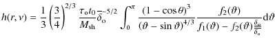
where
As remarked by Del Popolo et al. (2001), the angular momentum obtained from
Eq. (36) is evaluated at the time of maximum expansion ![]() .
With the BBKS power spectrum (filtered on a galactic scale),
for a
.
With the BBKS power spectrum (filtered on a galactic scale),
for a ![]() peak of mass
peak of mass ![]()
![]() ,
the model gives a value of
,
the model gives a value of
![]()
![]() .
.
It is interesting to compare this result with a different method such as that of Catelan & Theuns (1996), who calculated the
angular momentum at maximum expansion time (see their Eqs. (31)-(32)) and compared it with previous theoretical
and observational estimates. Assuming the same value of mass and ![]() used to obtain our previously quoted result
and the same distribution of angular momentum
as adopted by Catelan & Theuns (1996), we obtain a value for the
angular momentum of
used to obtain our previously quoted result
and the same distribution of angular momentum
as adopted by Catelan & Theuns (1996), we obtain a value for the
angular momentum of
![]()
![]() in agreement with our result.
in agreement with our result.
The total angular momentum of a system is often expressed in terms of the dimensionless spin parameter
 |
(37) |
where L is the angular momentum, summed over shells, and E is the binding energy of the halo. Expressing the values of angular momentum calculated as previously reported in terms of the spin parameter, we get a value of
Since our paper deals also with LSB galaxies, we recall that LSB galaxies are more angular-momentum-dominated than normal galaxies of the same luminosity (McGaugh & de Blok 1998). These galaxies are characterized by high values of ![]() ,
since, as shown in Boissier et al. (2002), 35% of all galaxies (in number) with
,
since, as shown in Boissier et al. (2002), 35% of all galaxies (in number) with
![]() are LSBs.
According to several analytical papers (Nusser 2001;
Hiotelis 2002;
Le Delliou & Henriksen 2003;
Ascasibar et al. 2004;
Williams et al. 2004), one therefore expects that these objects should typically have shallower density cusps. Moreover the cores of these galaxies are also much less dense than the simulations indicate.
In the case of LSB galaxies, we assumed a value of
are LSBs.
According to several analytical papers (Nusser 2001;
Hiotelis 2002;
Le Delliou & Henriksen 2003;
Ascasibar et al. 2004;
Williams et al. 2004), one therefore expects that these objects should typically have shallower density cusps. Moreover the cores of these galaxies are also much less dense than the simulations indicate.
In the case of LSB galaxies, we assumed a value of
![]() as a conservative estimate.
In agreement with what has been reported, larger values of
as a conservative estimate.
In agreement with what has been reported, larger values of ![]() should correspond to additional
flattening of the rotation curves in Fig. 4.
A more complete description of this calculation can be found in Del Popolo (2006).
should correspond to additional
flattening of the rotation curves in Fig. 4.
A more complete description of this calculation can be found in Del Popolo (2006).
We note that after turnaround, not only the random angular momentum, j, will contribute to the non-radial motions in the protostructure but also the ordered angular momentum, h. In fact, as successive shells expand to their maximum radius, they acquire angular momentum and then collapse on orbits determined by their angular momentum. Actual peaks are not spherical, thus the infall of matter will not be purely radial. Random substructure in the region surrounding the peak will divert infalling matter onto non-radial orbits. The role of these random motions is of fundamental importance to structure formation.
Dynamical friction was taken into account by introducing the dynamical friction force to the equation of motions. In ordered to calculate ![]() ,
we recall that in hierarchical universes, matter is concentrated in lumps, and the lumps into groups and so on, which act as gravitational field generators. One can calculate the stochastic force generated by these field generators and then following Kandrup (1980) the dynamical friction force per unit mass
,
we recall that in hierarchical universes, matter is concentrated in lumps, and the lumps into groups and so on, which act as gravitational field generators. One can calculate the stochastic force generated by these field generators and then following Kandrup (1980) the dynamical friction force per unit mass
![$\displaystyle -\mu v=-\frac{4.44[Gm_{\rm a}n_{\rm ac}]^{1/2} \log \left( 1.12N^{2/3}\right)}N \frac v{a^{3/2}}$](/articles/aa/full_html/2009/30/aa11404-08/img141.png)
where
| r(ri,t)=ria(ri,t). | (39) |
The number and mass of the field generators is then calculated using the theory of Gaussian random fields (BBKS). The acceleration obtained from Eq. (38) is used in the equation of motion. The reader is again referred to Del Popolo (2006) for a more complete description.
The shape of the central density profile is influenced by baryonic collapse: baryons drag dark matter in, causing the so-called adiabatic contraction (AC) and a steepening of the dark matter density slope.
By considering a spherically symmetric protostructure, before dissipation, that consists of a baryonic fraction F
with ![]() of dissipational baryons and a fraction 1-F of dissipationless dark matter particles constituting the halo, Blumenthal et al. (1986)
described an approximate analytical model to calculate the effects of AC.
One assumes that the dissipational baryons and the halo particles are well mixed initially (i.e., the ratio of their densities is F throughout
the protostructure).
This is because the original angular momentum of the dark matter halo comes from gravitational (tidal) interactions
with its environment. Thus, the dark matter and gas experience the same torque in the process of halo assembly and should initially have (almost) the same specific angular momentum (Klypin et al. 2002).
A usual assumption is, therefore, that initially baryons had the same density profile as the dark matter (see the previous discussion and Mo et al. 1998; Cardone & Sereno 2005;
Treu & Koopmans 2002; Keeton 2001).
of dissipational baryons and a fraction 1-F of dissipationless dark matter particles constituting the halo, Blumenthal et al. (1986)
described an approximate analytical model to calculate the effects of AC.
One assumes that the dissipational baryons and the halo particles are well mixed initially (i.e., the ratio of their densities is F throughout
the protostructure).
This is because the original angular momentum of the dark matter halo comes from gravitational (tidal) interactions
with its environment. Thus, the dark matter and gas experience the same torque in the process of halo assembly and should initially have (almost) the same specific angular momentum (Klypin et al. 2002).
A usual assumption is, therefore, that initially baryons had the same density profile as the dark matter (see the previous discussion and Mo et al. 1998; Cardone & Sereno 2005;
Treu & Koopmans 2002; Keeton 2001).
In real systems, baryons assume a distribution in the central regions of the halo determined by the competition between dissipation and star formation. The dissipative infall of baryons ceases either when most of the baryon gas is converted into stars, ending dissipation, or when a rotationally supported gas disk is formed. As the baryons dissipate energy, they fall toward the center of the halo. If the baryons conserve their angular momentum as they fall inward, then the baryons will dissipate energy until they form a rotationally supported disk, whose shape is determined by the angular momentum distribution h(M) of the baryons. Summarizing, the two methods for halting dissipative infall produce a spheroidal distribution (if star formation ends the infall) or in a disk of stars (if angular momentum ends the infall) (R88a). Following usual practice, the final baryon distribution is assumed to be a disk for spiral galaxies (Blumenthal et al. 1986; Flores et al. 1993; Mo et al. 1998; Klypin et al. 2002; Cardone & Sereno 2005). In our calculations, we shall assume the Klypin et al. (2002) model for the baryon distribution (see their Sect. 2.1), when dealing with mass scales typical of spiral galaxies. In the case of elliptical galaxies and clusters, a typical assumption (that we use in this paper) is that baryons collapse to a Hernquist configuration (Rix et al. 1997; Keeton 2001; Treu & Koopmans 2002). One objection that one could advance is that clearly if the final baryon distribution is assumed to be a disk, the inner gravity potential is clearly non-spherical. The usual assumption that is made at this step (see RG87; R88a,b; Mo et al. 1998; Klypin et al. 2001; Cardone et al. 2006) is that the final configuration (in this case the disk) is assembled slowly, so that we can assume that the halo responds adiabatically to the modification of the gravitational potential and remains spherical while contracting. The angular momentum of the dark matter particles is then conserved and a particle that is initially at radius r, ends up at a radius r', as described in the following.
The scale of the Hernquist profile is fixed by the competition between dissipation and star formation, when most of the baryon gas is converted into stars (see RG87; Gnedin et al. 2004).
As achieved by RG87, we take into account adiabatic compression improving its description as outlined
by Gnedin et al. (2004, see the following).
The Blumenthal et al. (1986), RG87, and R88ab models of adiabatic contraction can be described as follows.
Since the baryon fraction F is much less than one, the adiabatic invariants of the dark matter orbits are conserved (Blumenthal et al. 1986; RG87). If the matter is on circular orbits, the invariant is r M(r); if the dark matter is on radial orbits in a self-similar distribution, the invariant is
![]() (Blumenthal et al. 1986). Since the actual orbits are neither circular nor radial, the two adiabatic invariants that are preserved are the angular momentum
(Blumenthal et al. 1986). Since the actual orbits are neither circular nor radial, the two adiabatic invariants that are preserved are the angular momentum ![]() and jr, of the orbits (RG87). In the absence of dissipation, the mass distribution M0(r) has a value of F, which is constant throughout the structure. A self-consistent final solution, in which the baryons form a disk (or Hernquist configuration), conserving h, and the dark matter is compressed, conserving
and jr, of the orbits (RG87). In the absence of dissipation, the mass distribution M0(r) has a value of F, which is constant throughout the structure. A self-consistent final solution, in which the baryons form a disk (or Hernquist configuration), conserving h, and the dark matter is compressed, conserving ![]() and jr, is found by an iterative procedure. In the zeroth-order approximation, the baryons have their predissipation distribution
and jr, is found by an iterative procedure. In the zeroth-order approximation, the baryons have their predissipation distribution
![]() ,
and the dark matter has the distribution
,
and the dark matter has the distribution
![]() .
While the dark matter distribution is held constant, the baryons fall inward, preserving their angular momentum until they are on circular orbits. Baryons originally at radius r and with specific angular momentum h will end up, in the stiff halo, at a radius,
.
While the dark matter distribution is held constant, the baryons fall inward, preserving their angular momentum until they are on circular orbits. Baryons originally at radius r and with specific angular momentum h will end up, in the stiff halo, at a radius,
![\begin{displaymath}r'=\frac{h^2}{G[M_{\rm B0}(r)+M_{\rm D0}(r')]}\cdot
\end{displaymath}](/articles/aa/full_html/2009/30/aa11404-08/img152.png) |
(40) |
The baryons now have a new, more compact distribution
 |
(41) |
After fixing the value of
![\begin{displaymath}r''=\frac{h^2}{G[M_{\rm B1}(r)+M_{\rm D1}(r'')]},
\end{displaymath}](/articles/aa/full_html/2009/30/aa11404-08/img158.png) |
(42) |
and the new potential
where the orbit-averaged radius is
 |
(44) |
where
![\begin{figure}
\subfigure[]{\includegraphics[width=8.5cm,clip]{11404fig1a.eps} }
\subfigure[]{\includegraphics[width=8.5cm,clip]{11404fig1b.eps} }\end{figure}](/articles/aa/full_html/2009/30/aa11404-08/img169.png) |
Figure 1:
Panel a) Dark matter haloes generated with the model of Sect. 2. In this case we do not take into account baryon collapse. The upper dashed-line represents the results of the Aquarius Experiment for a halo of
|
| Open with DEXTER | |
The universal baryon fraction has been inferred by observations involving different physical processes (Turner 2002). The power spectrum of matter inhomogeneities in large-scale structure is sensitive to the quoted F; the Two Degree Field Galaxy Redshift Survey reported a value of
![]() (Percival et al. 2001). Measurements of the angular power spectrum of the CMBR also provided a very significant estimate. The combined analysis in Jaffe et al. (2001) of several data sets gives
F= 0.186+0.010-0.008. By using WMAP collaboration data (Spergel et al. 2003), one obtains
(Percival et al. 2001). Measurements of the angular power spectrum of the CMBR also provided a very significant estimate. The combined analysis in Jaffe et al. (2001) of several data sets gives
F= 0.186+0.010-0.008. By using WMAP collaboration data (Spergel et al. 2003), one obtains
![]() (
(
![]() ;
;
![]() ). After baryons cool and form stars, the baryon-to-total mass at the virial radius
does not need to equal the previous quoted universal baryon fraction and may deviate from it depending on feedback effects, hierarchical formation details, and heating by the extragalactic UVB flux.
In the AC calculation, one has to take into account that for large galaxies, only about half of the baryons, in principle available within the virial radius, goes into the central galaxy. For dwarf galaxies, this amount may be much smaller because of
feedback effects, hierarchical formation details, and heating by the extragalactic UVB flux.
In the following, in the case of large galaxies, we use one half of the universal baryonic fraction, and for dwarfs, values obtainable from Hoeft et al. (2007) (their Fig. 1). For example, in the case of a dwarf galaxy of
). After baryons cool and form stars, the baryon-to-total mass at the virial radius
does not need to equal the previous quoted universal baryon fraction and may deviate from it depending on feedback effects, hierarchical formation details, and heating by the extragalactic UVB flux.
In the AC calculation, one has to take into account that for large galaxies, only about half of the baryons, in principle available within the virial radius, goes into the central galaxy. For dwarf galaxies, this amount may be much smaller because of
feedback effects, hierarchical formation details, and heating by the extragalactic UVB flux.
In the following, in the case of large galaxies, we use one half of the universal baryonic fraction, and for dwarfs, values obtainable from Hoeft et al. (2007) (their Fig. 1). For example, in the case of a dwarf galaxy of
![]() it is about 0.06.
it is about 0.06.
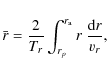
3 Results and discussion
After fixing the initial conditions and describing how to calculate angular momentum, dynamical friction, and adiabatic contraction, we can use
the model in Sect. 2 to obtain the density profile of haloes.
In Fig. 1, we plot the profiles obtained with our model and those predicted by numerical simulations.
In Fig. 1, the short-dashed line, the dashed line, and the solid line represents, respectively, the density profile for haloes of
![]() ,
,
![]() ,
and
,
and
![]() calculated by means of the model of this paper.
In order to compare the results of the model with those of N-body simulations, we plotted
the NFW profile (dot-dashed line) for haloes with masses equal to
calculated by means of the model of this paper.
In order to compare the results of the model with those of N-body simulations, we plotted
the NFW profile (dot-dashed line) for haloes with masses equal to
![]() ,
and c=10, and the results for the same mass
obtained in the Aquarius Project by Navarro et al. (2008)
(upper dashed-lines). Navarro et al. (2008) showed that density profiles deviate slightly but systematically from
the NFW model, and are approximated more accurately by a fitting formula where the logarithmic slope is a power-law of radius, the Einasto profile
,
and c=10, and the results for the same mass
obtained in the Aquarius Project by Navarro et al. (2008)
(upper dashed-lines). Navarro et al. (2008) showed that density profiles deviate slightly but systematically from
the NFW model, and are approximated more accurately by a fitting formula where the logarithmic slope is a power-law of radius, the Einasto profile
| (45) |
where r-2 and
Density profiles become monotonically shallower inwards, down to the innermost resolved point, with no indication that they approach power-law behavior. The innermost slope they measure is slightly shallower than -1, a result supported by estimates of the maximum possible asymptotic inner slope. Shallower cusps, such as the r-0.75 behavior predicted by the model of Taylor & Navarro (2001), cannot yet be excluded. Similarly, Graham et al. (2006) showed that Einasto and Prugniel-Simien models describe simulated dark matter halos better than a NFW model. A comparison of the quoted models with data from real galaxies gives an extrapolated inner (0.01-1 kpc) logarithmic profile slope ranging from approximately -0.2 to approximately -1.5, with a typical value at 0.1 kpc around -0.7.
The NFW profile for the given mass was calculated by means of the relationships connecting the concentration parameter, c, and the virial mass, ![]() ,
to the shape of NFW profile.
We used the following equation for c
,
to the shape of NFW profile.
We used the following equation for c
(Gentile et al. 2007), and the usual one for the NFW profile,
where
and
 |
(49) |
(Gentile et al. 2007). The residuals from the most robust Einasto fits are extremely small, and show no sign of systematic deviations down to the innermost resolved point. NFW residuals are then less than 30% over the full radial range and below 20% within r-2.
Figure 1 shows that halos generated using our method are different in character from the
profiles predicted by numerical simulations, such as those of NFW or the Aquarius project.
This result is unsurprising
since the types of evolution that numerical N-body and our halos undergo are rather different:
the former are produced as a cumulative result of many minor and major mergers of smaller
sub-halos, while the latter are the product of quiescent accretion of lumpy matter onto the
primary halo.
The NFW profiles change slope dramatically from ![]() to
to ![]() at the characteristic radius
at the characteristic radius ![]() .
For example, in the case of the
.
For example, in the case of the
![]() ,
the NFW profile has a characteristic scale length, equal to
,
the NFW profile has a characteristic scale length, equal to
![]() ,
beyond which the density profile steepens, so that much of the mass accumulates within 10% of the virial radius.
We note that Navarro et al. (2004), Stadel et al. (2008), and the Aquarius Experiment start to show that
the spherically-averaged density profile is not described, as in the NFW model, by just an outer power-law
,
beyond which the density profile steepens, so that much of the mass accumulates within 10% of the virial radius.
We note that Navarro et al. (2004), Stadel et al. (2008), and the Aquarius Experiment start to show that
the spherically-averaged density profile is not described, as in the NFW model, by just an outer power-law
![]() and inner power-law
and inner power-law
![]() ,
but becomes progressively shallower inwards, and at the innermost resolved radius, the logarithmic slope is
,
but becomes progressively shallower inwards, and at the innermost resolved radius, the logarithmic slope is
![]() ,
ruling out claims of a steep
,
ruling out claims of a steep
![]() central cusp, and not excluding shallower cusps as given by
the r-0.75 behavior predicted by the model of Taylor & Navarro (2001). In other words, simulations of higher resolution
are merging to the conclusion that the inner slope is not
so steep as it appeared in older simulations and so in some cases even marginally consistent
the DM halo of NGC 4605 (
central cusp, and not excluding shallower cusps as given by
the r-0.75 behavior predicted by the model of Taylor & Navarro (2001). In other words, simulations of higher resolution
are merging to the conclusion that the inner slope is not
so steep as it appeared in older simulations and so in some cases even marginally consistent
the DM halo of NGC 4605 (
![]() )
(Simon et al. 2003). In the following, we discuss another reason why density profiles obtained in N-body simulations differ from those obtained in our model.
)
(Simon et al. 2003). In the following, we discuss another reason why density profiles obtained in N-body simulations differ from those obtained in our model.
NFW profiles change slope rapidly from ![]() to
to ![]() at the characteristic radius
at the characteristic radius ![]() .
For example, in the case of the
.
For example, in the case of the
![]() model, the NFW profile has a characteristic scale length, equal to
model, the NFW profile has a characteristic scale length, equal to
![]() ,
beyond which the density profile steepens, so that much of the mass accumulates within 10% of the virial radius.
The haloes obtained using the model in Sect. 2 differ in character from the profiles predicted by numerical simulations, such as those of NFW.
Within the virial radius the log-log density slope changes gradually and the slopes of the inner part of haloes flatten with decreasing mass.
Our results show a steepening of the density profile with increasing mass of slopes
,
beyond which the density profile steepens, so that much of the mass accumulates within 10% of the virial radius.
The haloes obtained using the model in Sect. 2 differ in character from the profiles predicted by numerical simulations, such as those of NFW.
Within the virial radius the log-log density slope changes gradually and the slopes of the inner part of haloes flatten with decreasing mass.
Our results show a steepening of the density profile with increasing mass of slopes
![]() for
for
![]() ,
and
,
and
![]() for
for
![]() .
The profiles with
.
The profiles with
![]() are fitted well
by a Burkert profile, which has been considered to be a good fit to the dark matter rotation curves inferred from observations (e.g., Salucci & Burkert 2000).
The functional form of this profile is characterized by
are fitted well
by a Burkert profile, which has been considered to be a good fit to the dark matter rotation curves inferred from observations (e.g., Salucci & Burkert 2000).
The functional form of this profile is characterized by
![\begin{displaymath}\rho(r)= \frac{\rho_{\rm o}}{(1+r/r_{\rm o})[1+(r/r_{\rm o})^2]},
\end{displaymath}](/articles/aa/full_html/2009/30/aa11404-08/img198.png) |
(50) |
where
 |
(51) |
In panel a of Fig. 1, we plot results for the model of this paper in the case baryonic infall is not taken into account, and in panel b when baryonic infall is taken into account. Comparing panels a and b, we observe that the presence of baryons leads to a steeper profile in agreement with previous studies (Blumenthal et al. 1986; Flores et al. 1993; Klypin et al. 2002; Gnedin et al. 2004; Gustafsson et al. 2006). It is important to note that the effect of baryonic infall is more evident at early redshifts, as shown in Fig. 4a. As shown in Fig. 4a, from z=3 to z=2 the profile becomes even steeper than the NFW cusp. Later, the effect of angular momentum and dynamical friction reduces the slope and erases the cusp. However, as shown in Fig. 1 the initial steepening of the profile remains visible in the profiles calculated by the model in the present paper (
The model of the present paper gives just one profile for a given halo mass. In reality, N-body simulations and analytical models that differ
from those of Ryden-Williams and that of this paper (e.g., the extended Press-Schechter formalism) predict an ensemble of profiles for a given halo mass, depending on the different formation histories.
For example,
using the extended Press-Schechter (EPS) conditional probabilities for halo progenitor masses one can construct detailed histories of the mass
assembly of dark matter haloes.
One is interested in computing the mass accretion histories (hereafter MAHs) of dark matter haloes, defined as
![]() ,
where M(z) is defined as the mass of the main progenitor halo, and M0 is the halo mass at z = 0.
One then defines the average mass accretion history
of a halo of mass M0 as
,
where M(z) is defined as the mass of the main progenitor halo, and M0 is the halo mass at z = 0.
One then defines the average mass accretion history
of a halo of mass M0 as
 |
(52) |
where the summation is over an ensemble of N random realizations (see van den Bosch & Frank 2002). One can then convert the mass growth curves M(z) in density profiles as for example shown by Nusser & Sheth (1999). The single profile that we obtain in the present paper must be considered to be the average profile of all simulations. Two important things must be noted: a) less massive haloes are less concentrated; b) the halo's inner slope is shallower for smaller mass.
The first point can be explained as follows: higher peaks (larger ![]() ), which are progenitors of more massive haloes, have greater density contrast at their center, and so shells do not expand far before beginning to collapse. This reduces j
and h and allows haloes to become more concentrated. An alternative explanation is connected to the quoted angular momentum-density anticorrelation demonstrated
by Hoffman (1986):
), which are progenitors of more massive haloes, have greater density contrast at their center, and so shells do not expand far before beginning to collapse. This reduces j
and h and allows haloes to become more concentrated. An alternative explanation is connected to the quoted angular momentum-density anticorrelation demonstrated
by Hoffman (1986):
![]() (and similarly for h). So, density peaks with low (high) values of
(and similarly for h). So, density peaks with low (high) values of ![]() acquire a larger (smaller) amount of angular momentum than high
acquire a larger (smaller) amount of angular momentum than high ![]() peaks and consequently the halo becomes less (more) concentrated. We note that the quoted trend of increased central concentration as a function of mass applies only to halos that started out as peaks in the density field smoothed by a fixed Rf scale. Our conclusions do not mean that, for example, clusters of galaxies should be
far more centrally concentrated
than galaxies, since different smoothing scales would apply in the two cases.
Point (b) can be explained in a similar way to (a), as described previously.
Less massive objects are generated by peaks of smaller
peaks and consequently the halo becomes less (more) concentrated. We note that the quoted trend of increased central concentration as a function of mass applies only to halos that started out as peaks in the density field smoothed by a fixed Rf scale. Our conclusions do not mean that, for example, clusters of galaxies should be
far more centrally concentrated
than galaxies, since different smoothing scales would apply in the two cases.
Point (b) can be explained in a similar way to (a), as described previously.
Less massive objects are generated by peaks of smaller ![]() ,
which acquire
more angular momentum (h and j). The angular momentum sets the shape of the density profile at the inner regions. For pure radial orbits, the core is dominated by particles from the outer shells. As the angular momentum increases, these particles remains closer to the maximum radius,
resulting in a shallower density profile.
Particles with smaller angular momentum will be able to enter the core but with a reduced radial velocity compared with the purely
radial SIM. For some particles, the angular momentum is so large that they will never fall into the core (their rotational kinetic energy causes them to become unbound). Summarizing, particles of larger angular momenta are prevented from coming close to the halo's center and so contributing to the central density, which has the effect of flattening the density profile.
This result agrees with
the previrialization conjecture (Peebles & Groth 1976;
Davis & Peebles 1977; Peebles 1990), according to which initial asphericities and tidal
interactions between neighboring density fluctuations induce
significant non-radial motions that oppose the collapse.
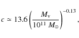
In order to reproduce the NFW profile, we performed an experiment similar to that performed by Williams et al. (2004), namely we
reduced the magnitude of the h and j angular momentum, dynamical friction,
,
which acquire
more angular momentum (h and j). The angular momentum sets the shape of the density profile at the inner regions. For pure radial orbits, the core is dominated by particles from the outer shells. As the angular momentum increases, these particles remains closer to the maximum radius,
resulting in a shallower density profile.
Particles with smaller angular momentum will be able to enter the core but with a reduced radial velocity compared with the purely
radial SIM. For some particles, the angular momentum is so large that they will never fall into the core (their rotational kinetic energy causes them to become unbound). Summarizing, particles of larger angular momenta are prevented from coming close to the halo's center and so contributing to the central density, which has the effect of flattening the density profile.
This result agrees with
the previrialization conjecture (Peebles & Groth 1976;
Davis & Peebles 1977; Peebles 1990), according to which initial asphericities and tidal
interactions between neighboring density fluctuations induce
significant non-radial motions that oppose the collapse.
In order to reproduce the NFW profile, we performed an experiment similar to that performed by Williams et al. (2004), namely we
reduced the magnitude of the h and j angular momentum, dynamical friction, ![]() ,
and we considered the system to consist
only of dark matter (F=0).
The experiment was performed on a halo of mass
,
and we considered the system to consist
only of dark matter (F=0).
The experiment was performed on a halo of mass
![]() ,
and to reproduce NFW profile with c=10 and mass
,
and to reproduce NFW profile with c=10 and mass
![]()
![]() ,
we had to reduce the magnitude of h by a factor of 2, and both j and
,
we had to reduce the magnitude of h by a factor of 2, and both j and ![]() by a factor of 2.5.
The result of this experiment is represented by the dashed line in Fig. 2, which closely reproduces the NFW profile (dot-dashed line),
and the dotted line is the profile for the
by a factor of 2.5.
The result of this experiment is represented by the dashed line in Fig. 2, which closely reproduces the NFW profile (dot-dashed line),
and the dotted line is the profile for the
![]() halo obtained by means of our model
halo obtained by means of our model![]() .
.
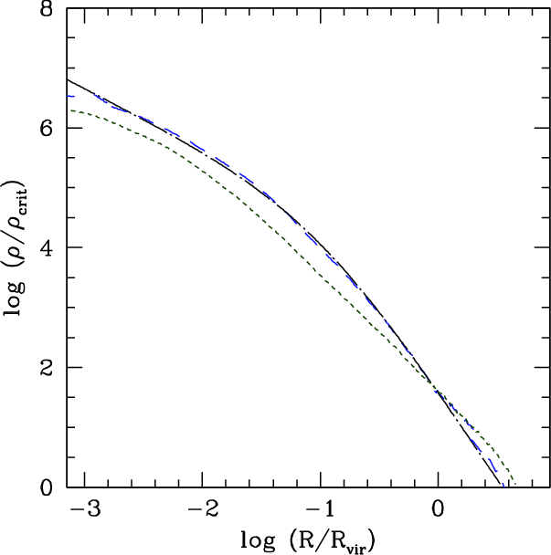 |
Figure 2:
Dark matter haloes generated with the model of Sect. 2. The dotted-dashed line is the NFW profile, the short-dashed line is the profile for the
|
| Open with DEXTER | |
Williams et al. (2004) similarly had to reduce the random velocities, which is equivalent to reducing the angular momentum, to obtain a NFW profile. After each reduction in the random velocities, the profiles became steeper at the center. This effect can be interpreted, as the central density being accumulated by shells whose pericenters are very close to the center of the halo. The correlation between increasing angular momentum and the reduction in the inner slopes of haloes has also been noted by several other authors (Avila-Reese et al. 1998, 2001; Subramanian et al. 1999; Nusser 2001; Hiotelis 2002; Le Delliou & Henriksen 2003; Ascasibar et al. 2004). As previously mentioned, there could be, according to Williams et al. (2004), another reason for the difference in density profiles obtained by N-body simulations and by models such as those in this paper (or William's). As shown in their Fig. 1 (lower-left panel), the specific angular momentum distribution (SAM) in NFW-like halo is more centrally concentrated than the SAM distribution of the reference halo obtained with their model, model which is similar to that of this paper, and is closer to those of typical halos emerging from numerical simulations. This may suggest, in agreement with Williams et al. (2004), that haloes in N-body simulations lose a considerable amount of angular momentum between 0.1 and 1 rv. Since virialization proceeds from inside out, this means that the angular momentum loss takes place during the later stages of the haloes' evolution, rather than very early on. This appears to be confirmed by the so-called angular momentum catastrophe, namely that dark matter halos generated by gas-dynamical simulations are too small and have too little angular momentum compared to the halos of real disk galaxies, possibly because it was lost during repeated collisions through dynamical friction or other mechanisms (van den Bosch et al. 2002; Navarro & Steinmetz 2000). The problem can be solved by introducing stellar feedback processes (Weil et al. 1998), but part of the angular momentum problem seems to be caused by numerical effects, most likely related to the shock-capturing, artificial viscosity used in smoothed particle hydrodynamics (SPH) simulations (Sommer-Larsen & Dolgov 2001).
We discussed the effect of changing the magnitude of angular momentum but did not consider the effect of changing the magnitude
of ![]() (dynamical friction), which is similar
to changing the magnitude of angular momentum:
an increase in the term
(dynamical friction), which is similar
to changing the magnitude of angular momentum:
an increase in the term ![]() produces shallower profiles
in much the same way
as larger values of angular momentum. This is expected from Del Popolo (2006)
(Fig. 1), showing that
dynamical friction influences the dynamics of collapse in a similar way to that
of angular momentum, slowing down the collapse of outer shells and compelling the particles to remain closer to the maximum radius.
produces shallower profiles
in much the same way
as larger values of angular momentum. This is expected from Del Popolo (2006)
(Fig. 1), showing that
dynamical friction influences the dynamics of collapse in a similar way to that
of angular momentum, slowing down the collapse of outer shells and compelling the particles to remain closer to the maximum radius.
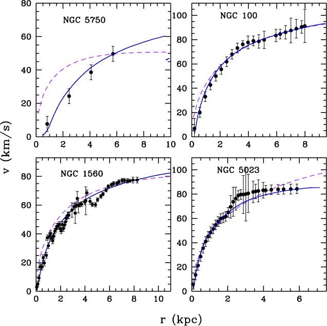 |
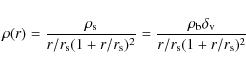
Figure 3: Comparison of the rotation curves obtained with the model in Sect. 2 (solid lines) with the rotation curves of four LSB galaxies studied by de Blok & Bosma (2002). The dashed line represents the fit with NFW model (see Sect. 3 for details). |
| Open with DEXTER | |
At this point, we emphasize that
the flattening of the density profile is caused by two main effects: angular momentum and dynamical friction. The other effect that we have considered, namely baryonic infall, counteracts the effect of the density profile flattening produced by angular momentum and dynamical friction. The role of baryonic infall is predominant at early times and produces a steepening of the profile, while at later times its effect is overwhelmed by the effect of angular momentum and dynamical friction.
The result is similar to that described by Williams et al. (2004), apart from that here
the effect of ordered angular momentum and dynamical friction adds to that of the random angular momentum studied by Williams et al. (2004),
producing a more significant
flattening of the density profiles.
In Fig. 3, we plot the rotation curves obtained by our model and we compare them to four LSB galaxies
taken from the high-resolution data of de Blok & Bosma (2002). Of the 26 LSBs that are
presented in that paper we picked the ones with high inclination angles, smooth rotation
curves, and good agreement between HI, Ha, and optical data.
In all four cases, the data are compared with
the rotation curve obtained using our model (solid line) and rotation curves obtained from the NFW profile (dotted lines), given by
![\begin{displaymath}V(r)=V_{\rm v}
\left \{
\frac{\ln (1+cx)-cx/(1+cx)}
{x [\ln(1+c)-c/(1+c)]}
\right \}^{1/2},
\end{displaymath}](/articles/aa/full_html/2009/30/aa11404-08/img211.png) |
(53) |
where
![$\displaystyle V(r)= \left
(\frac{2 \pi G \rho_0 r_{\rm o}^3}{r} \right)^{1/2}
\...
...rm o}) \sqrt(1+(r/r_{\rm o})^2)
\right]-
\arctan (r/r_{\rm o})
\right \}^{1/2},$](/articles/aa/full_html/2009/30/aa11404-08/img215.png) |
(54) |
Our rotation curves are very similar to those generated by the Burkert profile and the residuals and discrepant points for our rotation curves are close to those given in Gentile et al. (2004) for the Burkert's fit to their data. Our haloes appear to be a closer match to the haloes of spiral and dwarf galaxies, than N-body haloes. This may indicate that the haloes of real late-type disk galaxies undergo a formation scenario similar to the one depicted by our method, i.e., collapse proceeds through a quiescent accretion of lumpy material and minor mergers, rather than through a merger-driven formation process characteristic of hierarchical models. Before going on, we notice that of the four rotation curves, NGC 100 seems to be almost equally well fitted by the two type of models. In some other cases, the difference between the NFW rotation curves and those of the present paper is even smaller than for NGC100 and so it would be worthwhile to discuss halo-to-halo scatter. During the hierarchical assembly of dark matter haloes, the inner regions of early virialized objects often survive accretion onto a larger system, thus giving rise to a population of subhaloes. Depending on their orbits and masses, these subhaloes therefore either merge, are disrupted, or survive to the present day. To fully describe, in a statistical sense, the non-linear distribution of mass in the Universe, it is essential that halo substructure is taken into account. These subhaloes appear ubiquitous in high resolution cosmological simulations and provide the source of fluctuations. One can study the evolution of halos under the influence of a generation of subhaloes, while real halos grow continuously by accretion and mergers. Fluctuations caused by subhaloes in parent halos are important for understanding the time evolution of dark matter density profiles and the halo-to-halo scatter of the inner cusp seen in recent ultrahigh resolution cosmological simulations. This scatter may be explained by subhalo accretion histories: when we allow for a population of subhaloes of varying concentration and mass, the total inner profile of dark matter can either steepen or flatten.
As noted in the introduction, while on galactic scales many studies predict central cores and it seems that the cusp/core problem
is a real problem that cannot be attributed to systematic errors in the data (de Blok et al. 2003), on cluster scales the situation is less clear with slopes ranging from
![]() (e.g., Sand et al. 2002,
2004) to
(e.g., Sand et al. 2002,
2004) to
![]() (Arabadjis et al. 2002).
In order to study the problem on cluster scales, we calculated the density profile evolution of dark matter and that of the total matter
distribution for a halo of
(Arabadjis et al. 2002).
In order to study the problem on cluster scales, we calculated the density profile evolution of dark matter and that of the total matter
distribution for a halo of ![]()
![]() .
We used the method of Sect. 2 to calculate the density profile and then we repeated the experiment shown in Sect. 3 to reproduce the NFW profile for the quoted mass that we considered as the initial condition
.
We used the method of Sect. 2 to calculate the density profile and then we repeated the experiment shown in Sect. 3 to reproduce the NFW profile for the quoted mass that we considered as the initial condition![]() .
We then evolved this profile using the method of Sect. 2 and taking the redshift dependence in the model into account using the technique described in Del Popolo (2001) (the reader is referred to the quoted paper for more details).
The goal was to study the evolution of a NFW profile similar to El-Zant et al. (2001, 2004), Tonini et al. (2006), and Romano-Diaz et al. (2008), in a way.
.
We then evolved this profile using the method of Sect. 2 and taking the redshift dependence in the model into account using the technique described in Del Popolo (2001) (the reader is referred to the quoted paper for more details).
The goal was to study the evolution of a NFW profile similar to El-Zant et al. (2001, 2004), Tonini et al. (2006), and Romano-Diaz et al. (2008), in a way.
Before showing the results, we recall that in real haloes angular momentum is lost in the final stages of collapse by the transfer of angular momentum from the subclumps to external material by dynamical friction (Quinn & Zurek 1988; R88b; Klypin et al. 2002).
Once the baryons condense to form stars and galaxies, they experience a dynamical friction force from the less massive dark matter particles as they move through the halo. Energy and angular momentum is transferred to dark matter, increasing its random motion. Moreover, angular momentum acquired
in the expansion phase gives rise to non-radial motions in the collapse phase.
The spherical approximation that we use, which ignores the possibility of large substructures forming, neglects the transfer of angular momentum by means of the interactions of subclumps![]() .
In the present paper, the effect of dynamical friction was taken into account as an additive term in the equation of motion, Eq. (33),
without changing the spherical symmetry of the problem as done by Peebles (1993) and Del Popolo (2006).
The effect of the dynamical friction term in the equation of motion is very similar to that of the term of angular momentum:
an increase in the term
.
In the present paper, the effect of dynamical friction was taken into account as an additive term in the equation of motion, Eq. (33),
without changing the spherical symmetry of the problem as done by Peebles (1993) and Del Popolo (2006).
The effect of the dynamical friction term in the equation of motion is very similar to that of the term of angular momentum:
an increase in the term ![]() produces shallower profiles in a similar way to larger values of angular momentum. This is expected from Fig. 1 of Del Popolo (2006), showing that dynamical friction influences the dynamics of collapse in a similar way to that of angular momentum slowing down the collapse of outer shells and so compelling the particles to remain closer to the maximum radius.
produces shallower profiles in a similar way to larger values of angular momentum. This is expected from Fig. 1 of Del Popolo (2006), showing that dynamical friction influences the dynamics of collapse in a similar way to that of angular momentum slowing down the collapse of outer shells and so compelling the particles to remain closer to the maximum radius.
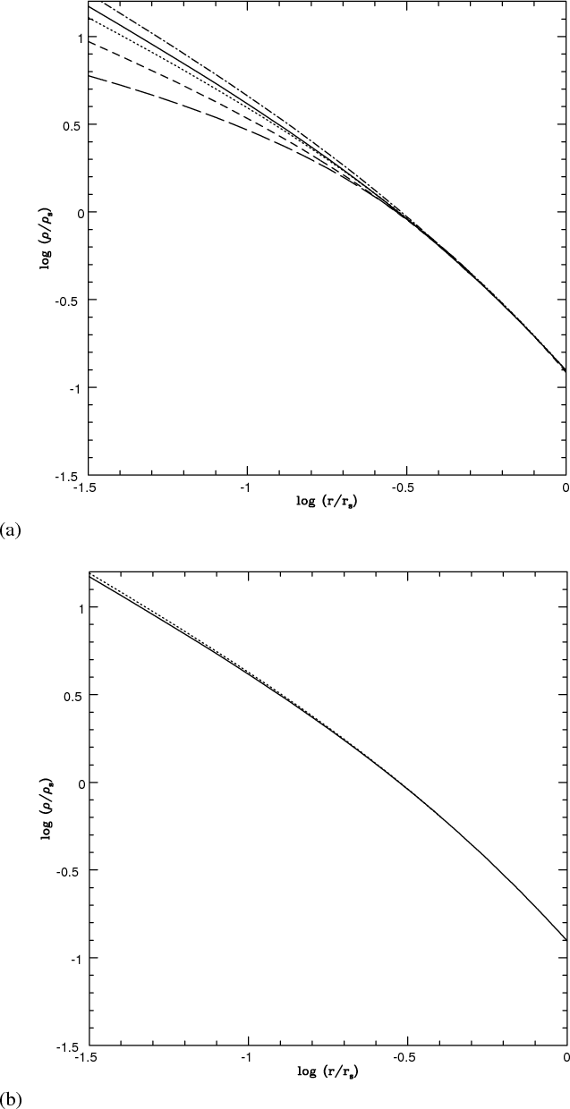 |
Figure 4:
Panel a) Density profile evolution of a
|
| Open with DEXTER | |
Figure 4a plots the evolution in a density profile of a mass
![]() .
The solid line represents the initial density profile at z=3, which subsequently steepens due to baryon settling in virialized dark matter haloes (AC) (dot-short-dashed line) at z=2.
Moreover, angular momentum acquired
in the expansion phase gives rise to non-radial motions in the collapse phase. The effect of angular momenta and dynamical friction overcomes that of the AC and the profile starts to flatten (z=1.5 dotted line; z=1 short-dashed line; z=0 long-dashed line). The final dark matter profile (long-dashed line) is characterized by a log-log slope of
.
The solid line represents the initial density profile at z=3, which subsequently steepens due to baryon settling in virialized dark matter haloes (AC) (dot-short-dashed line) at z=2.
Moreover, angular momentum acquired
in the expansion phase gives rise to non-radial motions in the collapse phase. The effect of angular momenta and dynamical friction overcomes that of the AC and the profile starts to flatten (z=1.5 dotted line; z=1 short-dashed line; z=0 long-dashed line). The final dark matter profile (long-dashed line) is characterized by a log-log slope of
![]() at
at
![]() .
The situation is therefore similar to that of haloes on galactic scales but the slope is steeper than for dwarf galaxies.
In Fig. 4b, we plot the evolution in the total density profile at initial redshift, z=3, (solid line) and at the final redshift z=0 (dotted line). The plot shows that the total density profile slightly changes
with time and the cusp is not ``erased'' as in the case of the dark matter profile. This result also implies that the baryonic component becomes steeper than the original NFW profile. The behavior of total mass agrees with that inferred from X-ray observations by Chandra and XMM (Buote 2003, 2004;
Lewis et al. 2003), weak lensing (Dahle et al. 2003), and strong lensing (Bartelmann 2003), which are consistent with a cusp of value
.
The situation is therefore similar to that of haloes on galactic scales but the slope is steeper than for dwarf galaxies.
In Fig. 4b, we plot the evolution in the total density profile at initial redshift, z=3, (solid line) and at the final redshift z=0 (dotted line). The plot shows that the total density profile slightly changes
with time and the cusp is not ``erased'' as in the case of the dark matter profile. This result also implies that the baryonic component becomes steeper than the original NFW profile. The behavior of total mass agrees with that inferred from X-ray observations by Chandra and XMM (Buote 2003, 2004;
Lewis et al. 2003), weak lensing (Dahle et al. 2003), and strong lensing (Bartelmann 2003), which are consistent with a cusp of value ![]() or larger. The behavior of the dark matter halo agrees with that inferred by the analysis of Sand et al. (2002, 2004),
who fitted the baryonic and dark matter profiles only in the very inner part of the cluster MS 2137-23 within
or larger. The behavior of the dark matter halo agrees with that inferred by the analysis of Sand et al. (2002, 2004),
who fitted the baryonic and dark matter profiles only in the very inner part of the cluster MS 2137-23 within ![]() 50 h-1 kpc with a generalized NFW profile
50 h-1 kpc with a generalized NFW profile
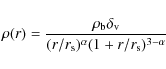 |
(55) |
obtaining a nearly flat core
The results previously reported have several implications on the effort to test predictions of the CDM model observationally. The test that has, as previously mentioned a number of times, is the density distribution in the inner regions of galaxies and clusters.
On galactic scales, as our results show, the infall of baryons at early times steepen the cusp because of AC (in agreement with previous studies: Blumenthal et al. 1986; Gnedin et al. 2004; Gustafsson et al. 2006), but later the cusp is erased by dynamical friction and non-radial motions effects. This results agree with other analyses that study separately the effects of dynamical friction (e.g., EZ01) and those of angular momentum (non-radial motions) (e.g., Nusser 2001; Hiotelis 2002; Ascasibar et al. 2004; Williams et al. 2004), and with the recent SPH simulations of Romano-Diaz et al. (2008).
On larger scales the situation is different. The analysis of the density distribution for bright galaxies is complicated by the uncertain contribution of stars to the total mass profile (Treu & Koopmans 2002; Mamon & Lokas 2004). Some analyses tend to favor inner slopes shallower than predicted by CDM (e.g., Gentile et al. 2004), but others measure inner profile slopes that are at least marginally consistent with predictions (Treu & Koopmans 2002, 2004; Koopmans & Treu 2003;
Jimenez et al. 2003).
As previously reported, our results exhibit a steepening in the density profile with increasing mass for a density profile of haloes of
![]() with slopes >0.8.
This agrees with recent N-body simulations having a
logarithmic slope that decreases inward more gradually than the NFW profile (Hayashi et al. 2003;
Navarro et al. 2004; Stadel et al. 2008).
In the case of Stadel et al. (2008) the logarithmic slope is 0.8 at
with slopes >0.8.
This agrees with recent N-body simulations having a
logarithmic slope that decreases inward more gradually than the NFW profile (Hayashi et al. 2003;
Navarro et al. 2004; Stadel et al. 2008).
In the case of Stadel et al. (2008) the logarithmic slope is 0.8 at ![]() of
of ![]() .
.
The density distribution of galaxy clusters can, in principle, provide a cleaner test of the models because the effects
of the baryons and gas on the dark matter distribution are expected to be smaller and simpler. However, in this case observations also predict slopes ranging from
![]() (
(
![]() ,
Sand et al. 2002, 2004) to values larger than one (Arabadjis et al. 2002) with in some cases different results being found for the same object. This is the case for the cluster MS2137-23 studied by Sand et al. (2004), who found a shallow density slope (
,
Sand et al. 2002, 2004) to values larger than one (Arabadjis et al. 2002) with in some cases different results being found for the same object. This is the case for the cluster MS2137-23 studied by Sand et al. (2004), who found a shallow density slope (![]() 0.5),
while Dalal & Keeton (2003), Bartelman & Meneghetti (2004) and Gavazzi (2003) contested Sand's results,
which according to them is neglecting lens ellipticity, and found consistency between the inner slope and NFW profile.
Our result on cluster scales differs for the dark matter and total mass distribution: the first tends to be less cuspy than the NFW profile in agreement with some observations (e.g., Sand et al. 2002, 2004), while the second is a bit more cuspy than the
NFW profile (in agreement with Brunzendorf & Meusinger 1999) .
0.5),
while Dalal & Keeton (2003), Bartelman & Meneghetti (2004) and Gavazzi (2003) contested Sand's results,
which according to them is neglecting lens ellipticity, and found consistency between the inner slope and NFW profile.
Our result on cluster scales differs for the dark matter and total mass distribution: the first tends to be less cuspy than the NFW profile in agreement with some observations (e.g., Sand et al. 2002, 2004), while the second is a bit more cuspy than the
NFW profile (in agreement with Brunzendorf & Meusinger 1999) .
In the present paper, we did not take into account the baryon-DM interaction. As previously reported, once the baryons condense to form stars and galaxies, energy and angular momentum is transferred to dark matter, increasing its random motion.
In future work,
we will develop a semianalytic
model to follow the evolution of the baryonic component, and its
interaction with DM, and we will compare these results with those of full hydrodynamical
simulations.
This should provide fresh insights into galaxy formation, and directly address possible small-scale
challenges to the CDM theory.
The role of the interaction between DM and baryons could bring further changes in the final density profile, which we shortly discuss.
We note that discrepancies between observations and
CDM only become apparent on length scales on which the
baryons begin to play a role not only for the cusp/core problem but
also for the missing dwarfs problem.
We also note that if, indeed, most
star-forming galaxies in the early universe lost their DM cusps because of stellar feedback, the
missing dwarfs (satellites) problem could also be solved. Dwarf galaxies without a central
cusp have a lower average core density than cuspy ones, and are hence much easier to disrupt
tidally during the hierarchical assembly of larger galaxies (Mashchenko & Sills 2005). As a
consequence, the removal of galactic cusps by stellar feedback in the early universe would
result in fewer satellites today (Mashchenko et al. 2006). This again indicates that baryon physics could be one of the missing
pieces of the puzzle, and will very likely make a major contribution toward a solution. If this
is true, it would be unwise to ignore the conclusions to which data are leading us, namely
that small scales tells us more about galaxy formation than it does about
CDM![]() . In other
words, the centers of galaxies are special places, the only places where we can study dark
matter under peculiar conditions.
. In other
words, the centers of galaxies are special places, the only places where we can study dark
matter under peculiar conditions.
4 Conclusions
In this paper, we have studied the cusp/core problem by improving the ESIM model of Williams et al. (2004).
We have taken into account, simultaneously, the effects of ordered and random angular momentum, dynamical friction and adiabatic contraction.
The improved SIM of the present paper, taking account the previous effects predicts haloes characterized by a log-log density slope that changes gradually within the virial radius and slopes of the inner haloes that flatten with decreasing mass. As in
previous papers, AC steepens the density profiles.
The density profiles of structure having masses smaller than
![]() are well fitted by Burkert profiles. The comparison of some of the rotational curves given by de Blok & Bosma (2002) with the rotational curves obtained by means of our model, provides a good agreement.
In the case of galaxy clusters, the density profile evolution is similar to that observed on galactic scales with the difference that the final slope is observed to be steeper than in the dwarf galaxies case. However, the total mass profile is still cuspy and evolves slightly with time.
The behavior of the dark matter halo is in agreement with the analysis of Sand et al. (2002, 2004), who fitted the baryonic and dark matter profiles only to the very inner part of the cluster MS 2137-23 within
are well fitted by Burkert profiles. The comparison of some of the rotational curves given by de Blok & Bosma (2002) with the rotational curves obtained by means of our model, provides a good agreement.
In the case of galaxy clusters, the density profile evolution is similar to that observed on galactic scales with the difference that the final slope is observed to be steeper than in the dwarf galaxies case. However, the total mass profile is still cuspy and evolves slightly with time.
The behavior of the dark matter halo is in agreement with the analysis of Sand et al. (2002, 2004), who fitted the baryonic and dark matter profiles only to the very inner part of the cluster MS 2137-23 within ![]() 50 h-1 kpc with a generalized NFW profile.
The behavior of the total mass is in agreement with X-ray observations by Chandra and XMM (Buote 2003, 2004;
Lewis et al. 2003) weak lensing (Dahle et al. 2003), and strong lensing (Bartelmann 2003), which are consistent with a cusp of
50 h-1 kpc with a generalized NFW profile.
The behavior of the total mass is in agreement with X-ray observations by Chandra and XMM (Buote 2003, 2004;
Lewis et al. 2003) weak lensing (Dahle et al. 2003), and strong lensing (Bartelmann 2003), which are consistent with a cusp of ![]() or of higher value.
As also reported by Williams et al. (2004), numerically generated halos must have lost a considerable amount of their angular momentum in the outer parts, roughly between 0.1 and
or of higher value.
As also reported by Williams et al. (2004), numerically generated halos must have lost a considerable amount of their angular momentum in the outer parts, roughly between 0.1 and
![]() ,
possibly by dynamical friction or other mechanisms.
A future model that takes into account the interaction between DM and baryons would help us to better understand the problem.
,
possibly by dynamical friction or other mechanisms.
A future model that takes into account the interaction between DM and baryons would help us to better understand the problem.
Acknowledgements
We would like to thank Massimo Ricotti, Nicos Hiotelis, and Antonaldo Diaferio for their very helpful suggestions and comments. Antonio Del Popolo acknowledges the financial support from the German Research Fondation (DFG) under grant NO KR 1635/16-1.
References
- Antonuccio-Delogu, V., & Colafrancesco, S. 1994, ApJ, 427, 72 [NASA ADS] [CrossRef] (ADC) (In the text)
- Arabadjis, J. S., Bautz, M. W., & Garmire, G. P. 2002, ApJ, 572, 66 [NASA ADS] [CrossRef] (In the text)
- Ascasibar, Y., Yepes, G., & Gottlober, S. 2004, MNRAS, 352, 1109 [NASA ADS] [CrossRef] (In the text)
- Ascasibar, Y., Hoffman, Y., & Gottlöber, S. 2007, MNRAS, 376, 393 [NASA ADS] [CrossRef] (In the text)
- Avila-Reese, V., Firmani, C., & Hernandez, X. 1998, ApJ, 505, 37 [NASA ADS] [CrossRef] (In the text)
- Bardeen, J. M., Bond, J. R., Kaiser, N., & Szalay, A. S. 1986, ApJ, 304, 15 [NASA ADS] [CrossRef] (In the text)
- Barnes, J., & Efstathiou, G. 1987, ApJ, 319, 575 [NASA ADS] [CrossRef] (In the text)
- Bartelmann, M. 2003, in Matter and Energy in Clusters of Galaxies, ASPC, 301, 255 (In the text)
- Bartelman, M., & Meneghetti, M. 2004, A&A, 418, 413 [NASA ADS] [CrossRef] [EDP Sciences] (In the text)
- Bertschinger, E. 1985, ApJS, 58, 39 [NASA ADS] [CrossRef] (In the text)
- Blumenthal, G. R., Faber, S. M., Flores, R., & Primack, J. R. 1986, ApJ, 301, 27 [NASA ADS] [CrossRef] (In the text)
- Boissier, S., Monnier, R. D., van Driel, W., Balkowski, C., & Prantzos, N. 2003, Ap&SS, 284, 913 [NASA ADS] [CrossRef]
- Borriello, A., & Salucci, P. 2001, MNRAS, 323, 285 [NASA ADS] [CrossRef] (In the text)
- Bothun, G., Impey, C., & McGaugh, S. 1997, PASP, 109, 745 [NASA ADS] [CrossRef] (In the text)
- Bryan, G. L., & Norman, M. L. 1998, ApJ, 495, 80 [NASA ADS] [CrossRef] (In the text)
- Bullock, J. S., Dekel, A., Kolatt, T. S., et al. 2001, ApJ, 555, 240 [NASA ADS] [CrossRef] (In the text)
- Brunzendorf, J., & Meusinger, H. 1999, A&AS, 139, 41 [NASA ADS] [CrossRef] (In the text)
- Buote, D. A. 2003, in IGM/Galaxy Connection, University of Colorado, ASSL Conf. Proc., 281, 87 (In the text)
- Buote, D. A. 2004, IAU Proc., 220, 149 (In the text)
- Burkert, A. 1995, ApJ, 447, L25 [NASA ADS] [CrossRef] (In the text)
- Cardone, V. F., & Sereno, M. 2005, A&A, 438, 545 [NASA ADS] [CrossRef] [EDP Sciences] (In the text)
- Catelan, P., & Theuns, T. 1996, MNRAS, 282, 436 [NASA ADS] (In the text)
- Cen, R. 2001, ApJ, 546, L77 [NASA ADS] [CrossRef] (In the text)
- Cen, R. Y., Dong, F., Bode, P., & Ostriker, J. P. 2004 [arXiv:astro-ph/0403352] (In the text)
- Cole, S., & Lacey, C. 1996, MNRAS, 281, 716 [NASA ADS] (In the text)
- Colin, P., Avila-Reese, V., & Valenzuela, O. 2000, ApJ, 542, 622 [NASA ADS] [CrossRef] (In the text)
- Dahle, H., Hannestad, S., & Sommer-Larsen, J. 2003, ApJ, 588, L73 [NASA ADS] [CrossRef] (In the text)
- Dalal, N., & Keeton, C. R. 2003 [arXiv:astro-ph/0312072] (In the text)
- Davé, R., Spergel, D. N., Steinhardt, P. J., & Wandelt, B. D. 2001, ApJ, 547, 574 [NASA ADS] [CrossRef] (In the text)
- Davis, M., & Peebles, P. J. E. 1977, ApJS, 34, 425 [NASA ADS] [CrossRef] (In the text)
- de Blok, W. J. G. 2003, in dark matter in Galaxies, ed. S. Ryder, D. J. Pisano, M. Walker, & K. C. Freeman, ASP Conf. Ser., 220,
- de Blok, W. J. G., & Bosma, A. 2002, A&A, 385, 816 [NASA ADS] [CrossRef] [EDP Sciences] (In the text)
- de Blok, W. J. G., McGaugh, S. S., Bosma, A., & Rubin, V. C. 2001a, ApJ, 552, L23 [NASA ADS] [CrossRef] (In the text)
- de Blok, W. J. G., McGaugh, S. S., & Rubin, V. C. 2001b, AJ, 122, 2396 [NASA ADS] [CrossRef]
- de Blok, W. J. G., Bosma, A., & McGaugh, S. 2003, MNRAS 340, 657 (In the text)
- Del Popolo, A. 2006, A&A, 454, 17 [NASA ADS] [CrossRef] [EDP Sciences] (In the text)
- Del Popolo, A., Gambera, M., Recami, E., & Spedicato, E. 2000, A&A, 353, 427 [NASA ADS] (DP2000) (In the text)
- Dubinski, J., & Carlberg, R. 1991, ApJ, 378, 496 [NASA ADS] [CrossRef] (In the text)
- Eisenstein, D. J., & Loeb, A. 1995, ApJ, 439, 250 [NASA ADS] [CrossRef] (In the text)
- El-Zant, A., Shlosman, I., & Hoffman, Y. 2001, ApJ, 560, 636 [NASA ADS] [CrossRef] (EZ01) (In the text)
- El-Zant, A., Hoffman, Y., Primack, J., Combes, F., & Shlosman, I. 2003, ApJ, 2004, ApJ, 607, 75 [CrossRef]
- Ettori, S., Fabian, A. C., Allen, S. W., & Johnstone, R. M. 2002, MNRAS, 331, 635 [NASA ADS] [CrossRef] (In the text)
- Filmore, J. A., & Goldreich, P. 1984, ApJ, 281, 1 [NASA ADS] [CrossRef]
- Flores, R. A., & Primack, J. R. 1994, ApJ, 427, L1 [NASA ADS] [CrossRef] (In the text)
- Flores, R., Primack, J. R., Blumenthal, G. R., & Faber, S. M. 1993, ApJ, 412, 443 [NASA ADS] [CrossRef] (In the text)
- Fukushige, T., & Makino, J. 2001, ApJ, 557, 533 [NASA ADS] [CrossRef] (In the text)
- Fukushige, T., Kawai, A., & Makino, J. 2004, ApJ, 606, 625 [NASA ADS] [CrossRef] (In the text)
- Gavazzi, R. 2003, in Impact of Gravitational Lensing on Cosmology, ed. Y. Mellier, & G. Meylan, Proc. IAU Symp., 225 (In the text)
- Gelato, S., & Sommer-Larsen, J. 1999, MNRAS, 303, 321 [NASA ADS] [CrossRef] (In the text)
- Gentile, G., Salucci, P., Klein, U., Vergani, D., & Kalberla, P. 2004, MNRAS, 351, 903 [NASA ADS] [CrossRef] (In the text)
- Gentile, G., Tonini, C., & Salucci, P. 2007, MNRAS, 378, 41 [NASA ADS] [CrossRef] (In the text)
- Ghigna, S., Moore, B., Governato, F., et al. 2000, ApJ, 544, 616 [NASA ADS] [CrossRef] (In the text)
- Gnedin, O. Y., Kravtsov, A. V., Klypin, A. A., & Nagai, D. 2004, ApJ, 616, 16 [NASA ADS] [CrossRef] (In the text)
- Goodman, J., 2000, New Astron., 5, 103 [NASA ADS] [CrossRef] (In the text)
- Gott, J. R. 1975, ApJ, 201, 296 [NASA ADS] [CrossRef] (In the text)
- Graham, A. W., Merritt, D., Moore, B., Diemand, J., & Terzic, B. 2006, AJ, 132, 2701 [NASA ADS] [CrossRef] (In the text)
- Gunn, J. E. 1977, ApJ, 218, 592 [NASA ADS] [CrossRef] (In the text)
- Gunn, J. E., & Gott, J. R. 1972, ApJ, 176, 1 [NASA ADS] [CrossRef] (In the text)
- Hayashi, E., Navarro, J. F., Power, C., et al. 2004, MNRAS, 355, 794 [NASA ADS] [CrossRef]
- Henriksen, R. N., & Widrow, L. M. 1999, MNRAS, 302, 321 [NASA ADS] [CrossRef] (In the text)
- Hiotelis, N. 2002, A&A 382, 84 (In the text)
- Hoeft, M., Mucket, J. P., & Gottlober, S. 2004, ApJ, 602, 162 [NASA ADS] [CrossRef]
- Hoffman, Y. 1986, ApJ, 301, 65 [NASA ADS] [CrossRef] (In the text)
- Hoffman, Y., & Shaham, J. 1985, ApJ, 297, 16 [NASA ADS] [CrossRef] (HS) (In the text)
- Hoyle, F. 1949, in IAU and International Union of Theorethicaland Applied Mechanics Symposium, 195 (In the text)
- Hozumi, S., Burkert, A., & Fujiwara, T. 2000, MNRAS, 311, 377 [NASA ADS] [CrossRef] (In the text)
- Hu, W., Barkana, R., & Gruzinov, A. 2000, Phys. Rev. Lett., 85, 1158 [NASA ADS] [CrossRef]
- Jimenez, R., Verde, L., & Oh, S. P. 2003, MNRAS, 339, 243 [NASA ADS] [CrossRef] (In the text)
- Jing, Y. P., & Suto, Y. 2000, ApJ, 529, L69 [NASA ADS] [CrossRef] (In the text)
- Kandrup, H. E. 1980, Phys. Rep., 63, 1 [NASA ADS] [CrossRef] (In the text)
- Kaplinghat, M., Knox, L., & Turner, M. S. 2000, Phys. Rev. Lett., 85, 3335 [NASA ADS] [CrossRef] (In the text)
- Kashlinsky, A. 1986, ApJ, 306, 374 [NASA ADS] [CrossRef] (In the text)
- Kashlinsky, A. 1987, ApJ, 312, 497 [NASA ADS] [CrossRef] (In the text)
- Keeton, C. R. 2001, ApJ, 561, 46 [NASA ADS] [CrossRef] (In the text)
- Klypin, A., Kravtsov, A. V., Bullock, James, S., & Primack, J. R. 2001, ApJ, 554, 903 [NASA ADS] [CrossRef] (In the text)
- Klypin, A., Zhao, H., & Somerville, R. S. 2002, ApJ, 573, 597 [NASA ADS] [CrossRef] (In the text)
- Koopmans, L. V. E., & Treu, T. 2003, ApJ, 583, 606 [NASA ADS] [CrossRef] (In the text)
- Kravtsov, A. V., Klypin, A. A., Bullock, J. S., & Primack, J. R. 1998, ApJ, 502, 48 [NASA ADS] [CrossRef] (In the text)
- Le Delliou, M., & Henriksen, R. N. 2003, A&A, 408, 27 [NASA ADS] [CrossRef] [EDP Sciences] (In the text)
- Lemson, G. 1995, Ph.D. Thesis, Rïksuniversiteit Groningen (In the text)
- Lewis, A. D., Buote, D. A., & Stocke, J. T. 2003, ApJ, 586, 135 [NASA ADS] [CrossRef] (In the text)
- Mamon, G. A., & Lokas, E. L. 2005, MNRAS, 362, 95 [NASA ADS] [CrossRef]
- Marchesini, D., D'Onghia, E., Chincarini, G., et al. 2002, ApJ, 575, 801 [NASA ADS] [CrossRef] (In the text)
- Mashchenko, S., Couchman, H. M. P., & Wadsley, J. 2006, Nature, 442, 539 [NASA ADS] [CrossRef] (In the text)
- Mashchenko, S., & Sills, A. 2005, ApJ, 619, 258 [NASA ADS] [CrossRef] (In the text)
- Merrit, D., Navarro, J. F., Ludlow, A., & Jenkins, A. 2005, ApJ, 624, L85 [NASA ADS] [CrossRef]
- Mo, H. J., Mao, S., & White, S. D. M. 1998, MNRAS, 295, 319 [NASA ADS] [CrossRef] (In the text)
- Moore, B. 1994, Nature, 370, 629 [NASA ADS] [CrossRef] (In the text)
- Moore, B., Governato, F., Quinn, T., Stadel, J., & Lake, G. 1998, ApJ, 499, L5 [NASA ADS] [CrossRef] (In the text)
- Navarro, J. F., Frenk, C. S., & White, S. D. M. 1995, MNRAS, 275, 720 [NASA ADS]
- Navarro, J. F., Frenk, C. S., & White, S. D. M. 1996, ApJ, 462, 563 [NASA ADS] [CrossRef] (In the text)
- Navarro, J. F., Frenk, C. S., & White, S. D. M. 1997, ApJ, 490, 493 [NASA ADS] [CrossRef] (NFW) (In the text)
- Navarro, J. F., Hayashi, E., Power, C., et al. 2004, MNRAS, 349, 1039 [NASA ADS] [CrossRef] (In the text)
- Nusser, A. 2001, MNRAS, 325, 1397 [NASA ADS] [CrossRef] (In the text)
- Nusser, A., & Sheth, R. K. 1999, MNRAS, 303, 685 [NASA ADS] [CrossRef] (In the text)
- Peebles, P. J. E. 1969, ApJ, 155, 393 [NASA ADS] [CrossRef] (In the text)
- Peebles, P. J. E. 1980, The large-scale structure of the Universe (Princeton University Press) (In the text)
- Peebles, P. J. E. 1990, ApJ, 365, 27 [NASA ADS] [CrossRef] (In the text)
- Peebles, P. J. E. 2000, ApJ, 534, L127 [NASA ADS] [CrossRef] (In the text)
- Peebles, P. J. E., & Groth, E. J. 1976, A&A, 53, 131 [NASA ADS] (In the text)
- Power, C., Navarro, J. F., Jenkins, A., et al. 2003, MNRAS, 338, 14 [NASA ADS] [CrossRef] (In the text)
- Quinn, P. J., Salmon, J. K., & Zurek, W. H. 1986, Nature, 322, 329 [NASA ADS] [CrossRef] (In the text)
- Rhee, G., Valenzuela, O., Klypin, A., Holtzman, J., & Moorthy, B. 2004, ApJ, 617, 1059 [NASA ADS] [CrossRef] (In the text)
- Ricotti, M. 2003, MNRAS, 344, 1237 [NASA ADS] [CrossRef]
- Ricotti, M., & Wilkinson, M. I. 2004, MNRAS, 353, 867 [NASA ADS] [CrossRef] (In the text)
- Ricotti, M., Pontzen, A., & Viel, M. 2007, ApJ, 663, 53 [NASA ADS] [CrossRef] (In the text)
- Rix, H.-W., de Zeeuw, P. T., Cretton, N., van der Marel, R. P., & Carollo, C. M. 1997, ApJ, 488, 702 [NASA ADS] [CrossRef] (In the text)
- Romano-Diaz, E., Shlosman, I., Hoffman, Y., & Heller, C. 2008 [arXiv:0808.0195] (In the text)
- Ryden, B. S. 1988a, ApJ, 329, 589 [NASA ADS] [CrossRef] (R88) (In the text)
- Ryden, B. S. 1988b, ApJ, 333, 78 [NASA ADS] [CrossRef]
- Ryden, B. S., & Gunn, J. E. 1987, ApJ, 318, 15 [NASA ADS] [CrossRef] (RG87) (In the text)
- Salucci, P., & Burkert, A. 2000, ApJ, 537, L9 [NASA ADS] [CrossRef] (In the text)
- Sand, D. J., Treu, T., & Ellis, R. S. 2002, ApJ, 574, L129 [NASA ADS] [CrossRef] (In the text)
- Sand, D. J., Treu, T., Smith, G. P., & Ellis, R. S. 2004, ApJ, 604, 88 [NASA ADS] [CrossRef] (In the text)
- Simon, J. D., Bolatto, A. D., Leroy, A., & Blitz, L. 2003, in Satellites and Tidal Streams, ASP Conf. Ser. (In the text)
- Sommer-Larsen, J., & Dolgov, A. 2001, ApJ, 551, 608 [NASA ADS] [CrossRef] (In the text)
- Spekkens, K., Giovanelli, R., & Haynes, M. P. 2005, AJ, 129, 2119 [NASA ADS] [CrossRef] (In the text)
- Spergel, D. N., & Steinhardt, P. J. 2000, Phys. Rev. Lett., 84, 3760 [NASA ADS] [CrossRef] (In the text)
- Spergel, D. N., Verde, L., Peiris, H. V., et al. 2003, ApJS, 148, 175 [NASA ADS] [CrossRef] (In the text)
- Stadel, J., Potter, D., Moore, B., et al. 2008 [arXiv:0808.2981] (In the text)
- Subramanian, K., Cen, R., & Ostriker, J. P. 2000, ApJ, 538, 528 [NASA ADS] [CrossRef] (In the text)
- Taylor, J. E., & Navarro, J. F. 2001, ApJ, 563, 483 [NASA ADS] [CrossRef] (In the text)
- Taylor, J. E., Silk, J., & Babul, A. 2004, IAU Symp., 220, 91 [NASA ADS] (In the text)
- Treu, T., & Koopmans, L. V. E. 2002, ApJ, 575, 87 [NASA ADS] [CrossRef] (In the text)
- Treu, T., & Koopmans, L. V. E. 2004, ApJ, 611, 739 [NASA ADS] [CrossRef] (In the text)
- van den Bosch, F. C., & Swaters, R. A. 2001, MNRAS, 325, 1017 [NASA ADS] [CrossRef] (In the text)
- van den Bosch, F. C., Robertson, B. E., Dalcanton, J. J., & de Blok, W. J. G. 2000, AJ, 119, 1579 [NASA ADS] [CrossRef] (In the text)
- Yoshida, N., Springel, V., White, S. D. M., & Tormen, G. 2000, ApJ, 544, L87 [NASA ADS] [CrossRef] (In the text)
- White, S. D. M. 1984, ApJ, 286, 38 [NASA ADS] [CrossRef] (In the text)
- White ,S. D. M., & Zaritsky, D. 1992, ApJ, 394, 1 [NASA ADS] [CrossRef] (In the text)
- Williams, L. L. R., Babul, A., & Dalcanton, J. J. 2004, ApJ, 604, 18 [NASA ADS] [CrossRef] (In the text)
Footnotes
- ... model
![[*]](/icons/foot_motif.png)
- A slightly overdense sphere, embedded in the Universe, is a useful non-linear model, as it behaves exactly as a closed sub-universe because of Birkhoff's theorem. The sphere is divided into spherical ``shells''. A spherical ``shell'' may be defined as the set of particles at a given radius that are all at the same phase in their orbits (see Le Delliou & Henriksen 2003).
- ...

 is the mass variance filtered on a scale Rf.
- ... Eq. (44)
- Note a typo in their paper:
 in the numerator of Eq. (44) should be
 .
.
- ... up
- In other words, the mass particles, once position and velocities are assigned, are allowed to follow the appropriate orbit in the gravitational
potential of the previously collapsed matter. As each mass shell is added, those previously added shells with which it overlaps have their orbits adjusted so that the angular momentum
 and radial moments jr integrated from pericenter to apocenter, are conserved.
- ...

- Notice that there is a very mild dependence of
 on peak height, or mass.
- ... model
- Note that the density profile of the Aquarius Experiment can be reproduced in the same manner with a small change in the h and j parameters used for the NFW profile.
- ... velocity
- The value of the characteristic velocity
 of the halo is defined in the same way as the virial radius
  .
.
- ... condition
- We could have started directly from a NFW profile for the given mass calculated by means of the NFW fitting formula.
- ... subclumps
- An approximate analytical approach to the problem of exchange of angular momentum between the dark matter particles and infalling baryons was developed by Klypin et al. (2002).
- ...
CDM
- Other possibilities are that the observed dark matter cores are telling us that dark matter has pressure at small scales or something unexpected.
All Figures
| |
Figure 1:
Panel a) Dark matter haloes generated with the model of Sect. 2. In this case we do not take into account baryon collapse. The upper dashed-line represents the results of the Aquarius Experiment for a halo of
|
| Open with DEXTER | |
| In the text | |
| |
Figure 2:
Dark matter haloes generated with the model of Sect. 2. The dotted-dashed line is the NFW profile, the short-dashed line is the profile for the
|
| Open with DEXTER | |
| In the text | |
| |
Figure 3: Comparison of the rotation curves obtained with the model in Sect. 2 (solid lines) with the rotation curves of four LSB galaxies studied by de Blok & Bosma (2002). The dashed line represents the fit with NFW model (see Sect. 3 for details). |
| Open with DEXTER | |
| In the text | |
| |
Figure 4:
Panel a) Density profile evolution of a
|
| Open with DEXTER | |
| In the text | |
Copyright ESO 2009
Current usage metrics show cumulative count of Article Views (full-text article views including HTML views, PDF and ePub downloads, according to the available data) and Abstracts Views on Vision4Press platform.
Data correspond to usage on the plateform after 2015. The current usage metrics is available 48-96 hours after online publication and is updated daily on week days.
Initial download of the metrics may take a while.