| Issue |
A&A
Volume 502, Number 3, August II 2009
|
|
|---|---|---|
| Page(s) | 721 - 731 | |
| Section | Cosmology (including clusters of galaxies) | |
| DOI | https://doi.org/10.1051/0004-6361/200811276 | |
| Published online | 15 June 2009 | |
Dependence of cosmic shear covariances on cosmology
Impact on parameter estimation
T. Eifler1 - P. Schneider1 - J. Hartlap1
Argelander-Institut für Astronomie, Universität Bonn, Auf dem Hügel 71, 53121 Bonn, Germany
Received 3 November 2008 / Accepted 16 April 2009
Abstract
Context. In cosmic shear likelihood analyses, the covariance is most commonly assumed to be constant in parameter space. Therefore, when calculating the covariance matrix (analytically or from simulations), its underlying cosmology should not influence the likelihood contours.
Aims. We examine whether the aforementioned assumptions hold and quantify how strong cosmic shear covariances vary within a reasonable parameter range. Furthermore, we examine the impact on likelihood contours when assuming different cosmologies in the covariance. The final goal is to develop an improved likelihood analysis for parameter estimation with cosmic shear.
Methods. We calculate Gaussian covariances analytically for 2500 different cosmologies. To quantify the impact on the parameter constraints, we perform a likelihood analysis for each covariance matrix and compare the likelihood contours. To improve on the assumption of a constant covariance, we use an adaptive covariance matrix, which is continuously updated according to the point in parameter space where the likelihood is evaluated. As a side-effect, this cosmology-dependent covariance improves the parameter constraints. We examine this more closely using the Fisher-matrix formalism. In addition, we quantify the impact of non-Gaussian covariances on the likelihood contours using a ray-tracing covariance derived from the Millennium simulation. In this ansatz, we return to the approximation of a cosmology-independent covariance matrix, and to minimize the error due to this approximation, we develop the concept of an iterative likelihood analysis.
Results. Covariances vary significantly within the considered parameter range. The cosmology assumed in the covariance has a non-negligible impact on the size of the likelihood contours. This impact increases with increasing survey size, increasing number density of source galaxies, decreasing ellipticity noise, and when taking non-Gaussianity into account. A proper treatment of this effect is therefore even more important for future surveys. In this paper, we present methods for taking cosmology-dependent covariances into account.
Key words: cosmology: large-scale structure of the Universe - methods: statistical - cosmology: theory - cosmology: cosmological parameters
1 Introduction
Cosmic shear, first detected in 2000 (Bacon et al. 2000; Wittman et al. 2000; Kaiser et al. 2000; van Waerbeke et al. 2000), has become an important tool in cosmology. Latest results (e.g., Hetterscheidt et al. 2007; van Waerbeke et al. 2005; Fu et al. 2008; Massey et al. 2007; Semboloni et al. 2006; Schrabback et al. 2007; Hoekstra et al. 2006) already indicate its great ability to constrain cosmological parameters, which will be enhanced in the future by large upcoming surveys like Pan-STARRS, KIDS, DES, Euclid or LSST. The improved quality of cosmic shear data must be accompanied by an accurate data analysis that is free of assumptions biasing the results. In this context, obtaining appropriate covariances is a crucial issue of a precision cosmology likelihood analysis. Several methods are suggested in the literature and have been applied to cosmic shear data. An analytic expression for covariances assuming a Gaussian shear field was derived in Schneider et al. (2002a) and confirmed in Joachimi et al. (2008), who used a power spectrum approach that significantly reduces the computational effort in the calculation. This analytic expression has been used for parameter estimation in many surveys (e.g., van Waerbeke et al. 2005,Semboloni et al. 2006; Hoekstra et al. 2006). However, the assumption of a Gaussian shear field breaks down on small scales; according to Kilbinger & Schneider (2005) and Semboloni et al. (2007) non-linear effects become important at angular scales ![]() 10 arcmin. To account for non-Gaussianity, Semboloni et al. (2007) invented a calibration factor which is derived from a comparison of Gaussian to ray-tracing covariances. An application of this method to real data can be found in Fu et al. (2008). A second approach is the derivation of the covariance matrix from the data (e.g., Hetterscheidt et al. 2007; Massey et al. 2007). Here, the covariance is calculated via field-to-field variation, which involves a separation of the data set into many independent subsamples. This might lead to a loss of information on large scales if the survey is insufficiently large. Third, one can estimate the covariance matrix from ray-tracing simulations, a method that circumvents the aforementioned loss in information. Although, the covariance in this method is again derived by field-to-field variation, we can choose a sufficiently large numerical simulation to create many independent subsamples of adequate size.
10 arcmin. To account for non-Gaussianity, Semboloni et al. (2007) invented a calibration factor which is derived from a comparison of Gaussian to ray-tracing covariances. An application of this method to real data can be found in Fu et al. (2008). A second approach is the derivation of the covariance matrix from the data (e.g., Hetterscheidt et al. 2007; Massey et al. 2007). Here, the covariance is calculated via field-to-field variation, which involves a separation of the data set into many independent subsamples. This might lead to a loss of information on large scales if the survey is insufficiently large. Third, one can estimate the covariance matrix from ray-tracing simulations, a method that circumvents the aforementioned loss in information. Although, the covariance in this method is again derived by field-to-field variation, we can choose a sufficiently large numerical simulation to create many independent subsamples of adequate size.
We note that the last two methods involve an estimation process in the determination of the covariance matrix, which means that the inverse is biased and one has to correct for this effect (Anderson 2003; Hartlap et al. 2007). Nevertheless, deriving covariance matrices from ray-tracing simulations seems to be a promising method because it preserves all the information in the data and in addition takes the non-Gaussianity of the shear field into account.
The analytic expression and the ray-tracing covariance assume a specific cosmological model in their derivation. To date, cosmic shear likelihood analyses have treated the covariance matrix as a constant in parameter space, hence the parameter constraints are assumed to be unaffected by the underlying cosmology. In this paper, we intend to check this assumption and if we find that it does not hold, to present an improved likelihood formalism for future surveys.
This paper is organized as follows. Section 2 summarizes the basic theoretical background of the cosmic shear two-point correlation function (2PCF) and its corresponding covariance. In Sect. 3, we derive a scaling relation for covariances, which can be used for a fast calculation of covariances for arbitrary cosmology. Furthermore, we examine how strongly the covariance depends on its underlying cosmological model. The impact on parameter constraints when assuming a fixed cosmology in the covariance is the subject of Sect. 4, whereas we present improvements on this assumption in Sect. 5. Here, we consider a likelihood analysis with an adaptive covariance matrix, i.e., the covariance is calculated individually for each point in parameter space where the likelihood is evaluated. In addition, we outline the concept of an iterative covariance matrix, i.e., several likelihood analyses are performed, where the covariance is updated in every iteration according to the maximum likelihood parameter set. Here, we also examine the impact of non-Gaussian covariances on the likelihood contours using a ray-tracing covariance matrix derived from the Millennium Simulation. We present our conclusions in Sect. 6.
2 Data vectors and covariances of cosmic shear
We briefly review the basics of the cosmic shear two-point correlation function and its corresponding covariance matrix. For more details of this topic, the reader is referred to Bartelmann & Schneider (2001), Schneider et al. (2002a), Schneider et al. (2002b), Kilbinger & Schneider (2004), and Joachimi et al. (2008).
To measure the shear signal, we define
![]() as the connecting vector of two points and specify tangential and cross-component of the shear
as the connecting vector of two points and specify tangential and cross-component of the shear ![]() as
as
 |
(1) |
where
![$\displaystyle \int^{\infty}_0 \frac{{\rm d}\ell\;\ell}{2\pi} ~ {J}_{0/4}(\ell \theta)~ ~\left[P_{\rm E}(\ell) \pm P_{\rm B}(\ell)\right],$](/articles/aa/full_html/2009/30/aa11276-08/img39.png)
where Jn denotes the nth order Bessel-function. We only consider E-modes, therefore we define
For the rest of this paper, we neglect the index
The pure shot noise term vanishes in case of C+- and only contributes to the diagonal of C++ and C-. It can be calculated as

where A denotes the solid angle of the data field,
The corresponding expressions for V and M using the 2PCF are derived in Schneider et al. (2002a). In this paper we only need the expressions for the mixed term, which read
![$\displaystyle M_{+-} = \frac{2 \sigma^2_\epsilon}{\pi A \bar n} \int_0^\pi {\rm...
...atop k \right) (-1)^k \vartheta^k_i ~ \vartheta^{4-k}_j \cos(k \varphi) \right]$](/articles/aa/full_html/2009/30/aa11276-08/img56.png)
where we denote
3 Variations in covariances with respect to cosmology
We select a two-dimensional parameter grid with 50 ![]() 50 gridpoints of
50 gridpoints of
![]() and
and
![]() .
For each grid point, we calculate a covariance analytically using Eqs. (5)-(10). The shear power spectra
.
For each grid point, we calculate a covariance analytically using Eqs. (5)-(10). The shear power spectra ![]() are obtained from the density power spectra
are obtained from the density power spectra ![]() by employing Limber's equation. To derive
by employing Limber's equation. To derive ![]() ,
we assume an initial Harrison-Zeldovich power spectrum (
,
we assume an initial Harrison-Zeldovich power spectrum (
![]() where
where
![]() )
with the transfer function from Efstathiou et al. (1992). For the calculation of the non-linear evolution, we use the fitting formula of Smith et al. (2003). Throughout this paper, we assume a flat universe and fix all cosmological parameters except
)
with the transfer function from Efstathiou et al. (1992). For the calculation of the non-linear evolution, we use the fitting formula of Smith et al. (2003). Throughout this paper, we assume a flat universe and fix all cosmological parameters except
![]() and
and ![]() ,
more precisely H0=0.73 and
,
more precisely H0=0.73 and
![]() .
These values for H0 and
.
These values for H0 and
![]() together with
together with
![]() and
and
![]() define our fiducial cosmological model (
define our fiducial cosmological model (
![]() ), which we have chosen to be similar to the cosmology of the Millennium Simulation (Springel et al. 2005) for a later comparison of Gaussian and ray-tracing covariances. We assume all source galaxies to be at redshift z0=1.0. Using a redshift distribution instead would not change our results qualitatively. In addition to cosmology, the covariance depends on survey parameters. The scaling relations given in Sect. 3 are generally valid and independent of survey parameters. For the likelihood analyses in Sects. 4 and 5, we choose, unless stated otherwise, an intrinsic ellipticity noise of
), which we have chosen to be similar to the cosmology of the Millennium Simulation (Springel et al. 2005) for a later comparison of Gaussian and ray-tracing covariances. We assume all source galaxies to be at redshift z0=1.0. Using a redshift distribution instead would not change our results qualitatively. In addition to cosmology, the covariance depends on survey parameters. The scaling relations given in Sect. 3 are generally valid and independent of survey parameters. For the likelihood analyses in Sects. 4 and 5, we choose, unless stated otherwise, an intrinsic ellipticity noise of
![]() ,
a number density of source galaxies of
,
a number density of source galaxies of
![]() (similar to the values of the Dark Energy survey), and a survey that covers A=900 deg2. The angular scale of the 2PCF data vector for which we calculate the covariances covers a range from 0.1 arcmin to 180 arcmin, which is divided into 50 logarithmic bins. The results of this section are limited by the accuracy of the non-linear fitting formula of Smith et al. (2003). It will be the subject of future work to refine the results presented here using an improved version of this fit-formula.
(similar to the values of the Dark Energy survey), and a survey that covers A=900 deg2. The angular scale of the 2PCF data vector for which we calculate the covariances covers a range from 0.1 arcmin to 180 arcmin, which is divided into 50 logarithmic bins. The results of this section are limited by the accuracy of the non-linear fitting formula of Smith et al. (2003). It will be the subject of future work to refine the results presented here using an improved version of this fit-formula.
3.1 A fast method for calculating covariances of arbitrary
 and
and

![\begin{figure}
\par\includegraphics[width=8.5cm,clip]{11276fg1.ps}
\end{figure}](/articles/aa/full_html/2009/30/aa11276-08/img70.png) |
Figure 1:
The dimensionless shear power spectrum
|
| Open with DEXTER | |
From Eqs. (9) and (10), one can directly see that the covariance matrix depends on the cosmological model, which depends in turn on the power spectrum ![]() .
Figure 1 illustrates the change in
.
Figure 1 illustrates the change in ![]() when varying only
when varying only
![]() ,
or
,
or ![]() ,
and both parameters simultaneously; we see that it increases with
,
and both parameters simultaneously; we see that it increases with
![]() as well as with
as well as with ![]() .
.
For a given cosmological model, we can calculate the covariance directly from Eqs. (5)-(10). Performing this calculation for many sets of parameters is time-consuming; hence we seek a scaling relation, which relates the covariances of an arbitrary cosmology
![]() to a reference model
to a reference model
![]() (
(
![]() being the fiducial cosmology described above). A basic theorem in statistics states (e.g., Anderson 2003) that if there is a relation between two data vectors
being the fiducial cosmology described above). A basic theorem in statistics states (e.g., Anderson 2003) that if there is a relation between two data vectors ![]() and
and ![]() such as
such as
![]() (
(![]() being a matrix), the relation between the covariances of
being a matrix), the relation between the covariances of ![]() and
and ![]() can be written as
can be written as
In this derivation,

where we can calculate the scaling matrices
| (16) |
In contrast to a covariance matrix, the 2PCF can be calculated extremely rapidly for many different cosmologies by means of Eq. (3). Hence, it would be a fast and convenient method to calculate the covariance for a reference cosmology and then apply Eq. (15) to obtain covariances for arbitrary cosmological parameters. Unfortunately, we cannot transfer this method directly to the cosmic shear case. We recall that the 2PCF is derived from the measured ellipticities of galaxies. Schneider et al. (2002b) demonstrate that the intrinsic ellipticity terms cancel out in the derivation of the 2PCF estimator, hence the 2PCF is defined only in terms of the shear. In contrast, the 2PCF covariance not only consists of terms originating from the shear, but has additional noise terms that originate from the intrinsic ellipticity of galaxies. The pure shot noise term in Eq. (8) is independent of cosmology and, as can be seen from Eqs. (11)-(13), the mixed term cannot be scaled with the relation in Eq. (15), which is quadratic in the 2PCF.
However, in the limit of a noise-free covariance, i.e., considering only the cosmic variance term, a scaling relation similar to Eq. (15) exists. We prove this explicitly below by, in particular, showing that the scaling matrices are independent of the ensemble average. The cosmic variance term can be calculated via Eq. (9). Cosmology is important only in terms of the power spectrum, hence the relation between
![]() and
and
![]() can be described as
can be described as
![]() .
Using this relation, we transform the cosmic variance term in Eq. (9) for given bins
.
Using this relation, we transform the cosmic variance term in Eq. (9) for given bins
![]() as follows
as follows
where we discretize the integral into a sum of
to rewrite Eq. (17) as
The mean value theorem guarantees that there exist values
where we consider the limit
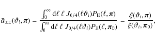
where we inserted Eq. (3) in the last step. This provides a fast and convenient method for scaling the cosmic variance term in parameter space, because we can use a computationally efficient Hankel transformation to calculate the 2PCF.
From Eqs. (11)-(13) we see that the mixed term
![]() scales linearly with the 2PCF, which prevents a scaling relation similar to Eq. (15). Fortunately, the direct calculation of the linear term with Eq. (10) is comparatively fast, and the scaling relation for the cosmic variance term therefore already reduces the computational costs significantly.
scales linearly with the 2PCF, which prevents a scaling relation similar to Eq. (15). Fortunately, the direct calculation of the linear term with Eq. (10) is comparatively fast, and the scaling relation for the cosmic variance term therefore already reduces the computational costs significantly.
Nonetheless, we numerically derive a fit-formula for the linear term based on the following expression
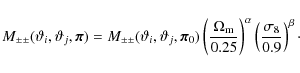
The structure of this fit-formula is motivated by the intention to use as few fit-parameters as possible; additionally we require that in the limit of the fiducial model,
3.2 Variations in the inverse covariance with respect to
and
From the variations in the power spectrum with
![]() and
and ![]() (Sect. 3.1), it is clear that covariances vary with respect to comological parameters. For simplicity and to improve the readability, we refer to this variation as the CDC-effect (CDC
(Sect. 3.1), it is clear that covariances vary with respect to comological parameters. For simplicity and to improve the readability, we refer to this variation as the CDC-effect (CDC ![]() Cosmology Dependent Covariances). To examine the CDC-effect more closely, we recall that the structure of the covariance is given by
Cosmology Dependent Covariances). To examine the CDC-effect more closely, we recall that the structure of the covariance is given by
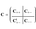 |
and the individual parts are calculated from Eqs. (5)-(10). From these equations, we can see that the covariances are filtered versions of the power spectrum, filtered either by a product of J0's (in the case of
To quantify the CDC-effect, we examine the trace of the inverse covariance matrix
![]() .
The trace of the covariance itself is an improper measure of this effect, as it depends on the binning, which can be seen from Eq. (8). The trace of
.
The trace of the covariance itself is an improper measure of this effect, as it depends on the binning, which can be seen from Eq. (8). The trace of ![]() becomes arbitrarily large when the bin width decreases. In contrast, we checked numerically that for the trace of
becomes arbitrarily large when the bin width decreases. In contrast, we checked numerically that for the trace of
![]() binning effects are negligible, once one has exceeded a minimum bin number. More precisely, once the bin width of the 2PCF data vector is small enough for discretization effects to be unimportant, the trace of
binning effects are negligible, once one has exceeded a minimum bin number. More precisely, once the bin width of the 2PCF data vector is small enough for discretization effects to be unimportant, the trace of
![]() hardly changes for different binning. For more details on how the binning affects covariances, their inverse, or parameter constraints derived from these covariances, the reader is referred to chapter 4 of ().
hardly changes for different binning. For more details on how the binning affects covariances, their inverse, or parameter constraints derived from these covariances, the reader is referred to chapter 4 of ().
![\begin{figure}
\par\includegraphics[width=8.5cm,clip]{11276fg2.ps}
\end{figure}](/articles/aa/full_html/2009/30/aa11276-08/img116.png) |
Figure 2:
The trace of the inverse covariance matrix
|
| Open with DEXTER | |
Figure 2 shows how the trace of the inverse covariance matrix depends on
![]() for various constant values of
for various constant values of ![]() (top) and vice versa (bottom). Here, we normalize the survey size to
(top) and vice versa (bottom). Here, we normalize the survey size to
![]() ,
and the other survey parameters are
,
and the other survey parameters are
![]() and
and
![]() .
We postpone a detailed analysis of how survey parameters influence the CDC-effect to Sect. 4. Qualitatively, the result does not change for different survey parameters; the trace of
.
We postpone a detailed analysis of how survey parameters influence the CDC-effect to Sect. 4. Qualitatively, the result does not change for different survey parameters; the trace of
![]() decreases with increasing
decreases with increasing
![]() or
or ![]() .
.
In addition, we perform a singular value decomposition (SVD) for each inverse covariance matrix. For the case of a symmetric and positive definite matrix, such as the inverse covariance matrix, an SVD yields the eigenvalues in decreasing order. For arbitrary i, we find that the ith eigenvalue decreases when increasing
![]() or
or ![]() .
The strength of the CDC-effect, i.e., the gradient of the traces, depends on the considered point in parameter space.
.
The strength of the CDC-effect, i.e., the gradient of the traces, depends on the considered point in parameter space.
4 Impact of the CDC-effect on parameter estimation
4.1 Basics of the likelihood analysis
Throughout the entire likelihood analysis, we assume the
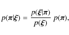
![]() model. We define the posterior likelihood
model. We define the posterior likelihood
![]() for the case of a 2PCF data vector as
for the case of a 2PCF data vector as
where
![\begin{displaymath}%
p({\vec \xi}\vert{\vec \pi}) = \frac{\exp ~ \left[ -\frac{1...
...t) \right]}{(2 \pi)^{d/2} \; \vert{\bf C}\vert^{\frac{1}{2}}},
\end{displaymath}](/articles/aa/full_html/2009/30/aa11276-08/img127.png)
where
![\begin{displaymath}%
p({\vec \xi})= \int {\rm d} {\vec \pi}~ \frac{\exp \left[- ...
...right]}{(2 \pi)^{d/2} \; \vert{\bf C}\vert^{\frac{1}{2}}}\cdot
\end{displaymath}](/articles/aa/full_html/2009/30/aa11276-08/img133.png)
In our case, we calculate
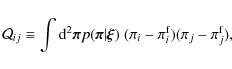
where
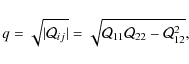
and can be considered as our figure-of-merit quantity. Smaller credible regions in parameter space correspond to a lower value of q. In this paper, all q are given in units of 10-4.
4.2 Results of the likelihood analysis
![\begin{figure}
\par\includegraphics[width=18cm,clip]{11276fg3.ps}
\end{figure}](/articles/aa/full_html/2009/30/aa11276-08/img140.png) |
Figure 3:
The 95%-credible intervals obtained from likelihood analyses with different cosmological models assumed in their covariance matrix. The left panel corresponds to the following covariance parameters:
|
| Open with DEXTER | |
In Sect. 3, we calculate 2500 covariances covering a parameter range of
![]() and
and
![]() .
We examine how the CDC-effect influences the likelihood contours, and hence, for each of the 2500 covariance matrices, we perform a likelihood analysis. In these analyses, we consider the same parameter space, similar priors, and similar
.
We examine how the CDC-effect influences the likelihood contours, and hence, for each of the 2500 covariance matrices, we perform a likelihood analysis. In these analyses, we consider the same parameter space, similar priors, and similar
![]() and
and
![]() ,
only the covariance in Eq. (25) is changed. The left panel of Fig. 3 shows the 95%-credible intervals when choosing
,
only the covariance in Eq. (25) is changed. The left panel of Fig. 3 shows the 95%-credible intervals when choosing
![]() and
and
![]() (solid),
(solid),
![]() ,
and
,
and
![]() (dotted) as a model for the covariance matrix. We compare these to the (dashed) case when the covariance is calculated from the fiducial model (
(dotted) as a model for the covariance matrix. We compare these to the (dashed) case when the covariance is calculated from the fiducial model (
![]() ,
,
![]() ). These examples illustrate that assuming different cosmologies in the covariance can significantly broaden or narrow the likelihood contours. As expected from the foregoing analysis of the inverse covariance traces (Sect. 3), the contours broaden for increasing
). These examples illustrate that assuming different cosmologies in the covariance can significantly broaden or narrow the likelihood contours. As expected from the foregoing analysis of the inverse covariance traces (Sect. 3), the contours broaden for increasing
![]() and
and ![]() .
.
Without any information about which cosmology to choose in our covariance matrix, it is reasonable to include prior information from other cosmological probes. The middle panel of Fig. 3 shows the 95% credible intervals when calculating the covariance from the minimum, mean, and maximum values of the 68% confidence region of the recent WMAP 5-year analysis (Komatsu et al. 2008). Compared to the left panel, the deviation in the contours reduces significantly, although it remains noticeable and cannot be neglected in a precision cosmology analysis. Similarly, the right panel shows the impact of the CDC-effect when calculating the covariance from parameters within the 95% confidence region of the recent WMAP5 analysis. We calculate the values of q (Sect. 4.1) for all contour plots and summarize them in Table 1. Restricting the possible cosmologies for the covariance to the 68% contour region of the WMAP5 analysis, the values of q deviate by a factor of
![]() .
This factor increases to
.
This factor increases to
![]() when considering the minimum and maximum values of the 95% confidence region of the WMAP5 constraints. In Fig. 4, we show the values of q for all 2500 likelihood analyses depending on
when considering the minimum and maximum values of the 95% confidence region of the WMAP5 constraints. In Fig. 4, we show the values of q for all 2500 likelihood analyses depending on
![]() (top) and
(top) and ![]() (bottom). Similar to the parameter dependence of the inverse covariances in Sect. 3, the strength of the CDC-effect, i.e., the gradient of the curves in Fig. 4, depends on the considered point in parameter space. For the fiducial model we calculate
(bottom). Similar to the parameter dependence of the inverse covariances in Sect. 3, the strength of the CDC-effect, i.e., the gradient of the curves in Fig. 4, depends on the considered point in parameter space. For the fiducial model we calculate
![]() and
and
![]() .
.
![\begin{figure}
\par\includegraphics[width=8.5cm,clip]{11276fg4.ps}
\end{figure}](/articles/aa/full_html/2009/30/aa11276-08/img145.png) |
Figure 4:
The values of q depending on
|
| Open with DEXTER | |
Table 1: Values of q for different covariance models.
4.3 Impact of survey parameters on the CDC-effect
![\begin{figure}
\par\includegraphics[width=8cm,clip]{11276fg5.ps}
\end{figure}](/articles/aa/full_html/2009/30/aa11276-08/img150.png) |
Figure 5:
The ratio of maximum to minimum value of q depending on the ratio
|
| Open with DEXTER | |
We have shown, that the CDC-effect non-negligibly affects the likelihood contours. However, we have only quantified this for one specific set of survey parameters. In this section, we examine how the impact of the CDC-effect on likelihood contours depends on survey parameters, namely the survey size A, the ellipticity dispersion
![]() ,
and the number density of source galaxies
,
and the number density of source galaxies ![]() ,
where in the case of the latter two, only the combination
,
where in the case of the latter two, only the combination
![]() is of interest. We perform likelihood analyses for 9 different combinations of
is of interest. We perform likelihood analyses for 9 different combinations of
![]() and 8 different survey sizes. The strength of the CDC-effect is quantified by the ratio of maximum to minimum value of q, which occur within the considered range of
and 8 different survey sizes. The strength of the CDC-effect is quantified by the ratio of maximum to minimum value of q, which occur within the considered range of
![]() and
and ![]() ,
defined to be
,
defined to be
![]() .
The minimum value of q is obtained when choosing the minimum parameter set in the calculation of the covariance, i.e.,
.
The minimum value of q is obtained when choosing the minimum parameter set in the calculation of the covariance, i.e.,
![]() .
Correspondingly, choosing the maximum parameter set
.
Correspondingly, choosing the maximum parameter set
![]() results in the maximal value of q. The values of q represent the size of credible intervals, hence
results in the maximal value of q. The values of q represent the size of credible intervals, hence ![]() can be interpreted as their ratio.
can be interpreted as their ratio.
Unfortunately, it is not possible to derive an analytical expression for the relation between ![]() and the survey parameters. From Eqs. (8)-(10) we see that the individual covariance terms scale differently with
and the survey parameters. From Eqs. (8)-(10) we see that the individual covariance terms scale differently with
![]() .
This already prohibits an analytically derived relation between
.
This already prohibits an analytically derived relation between ![]() and
and
![]() .
Considering the survey size A, Eqs. (8)-(10) imply that the total covariance scales with 1/A. When comparing two (inverse) covariances with different cosmologies by taking their ratio, the survey size cancels, suggesting that the strength of CDC-effect is independent of A. However, when considering the likelihood, the inverse covariance enters in the exponent, and the values of q are furthermore an integral over the posterior likelihood. This non-linearity in the inverse covariance causes the strength of the CDC-effect to vary with the survey size. An analytic expression of this dependence cannot be derived, for similar reasons as for the case of
.
Considering the survey size A, Eqs. (8)-(10) imply that the total covariance scales with 1/A. When comparing two (inverse) covariances with different cosmologies by taking their ratio, the survey size cancels, suggesting that the strength of CDC-effect is independent of A. However, when considering the likelihood, the inverse covariance enters in the exponent, and the values of q are furthermore an integral over the posterior likelihood. This non-linearity in the inverse covariance causes the strength of the CDC-effect to vary with the survey size. An analytic expression of this dependence cannot be derived, for similar reasons as for the case of
![]() .
We therefore calculate
.
We therefore calculate ![]() depending on the survey parameters numerically.
depending on the survey parameters numerically.
The upper panel of Fig. 5 shows
![]() as a function of
as a function of
![]() .
The ratio
.
The ratio ![]() changes from 4 to 18 over the considered interval of
changes from 4 to 18 over the considered interval of
![]() .
When increasing the survey size A (Fig. 5, lower panel), we find that the impact of the CDC-effect increases from
.
When increasing the survey size A (Fig. 5, lower panel), we find that the impact of the CDC-effect increases from
![]() (for a 25 deg2 survey) to
(for a 25 deg2 survey) to
![]() (for a 2500 deg2 survey). We note that the size of the likelihood contours, and hence the values of q themselves, decrease with decreasing
(for a 2500 deg2 survey). We note that the size of the likelihood contours, and hence the values of q themselves, decrease with decreasing
![]() and increasing A. In contrast,
and increasing A. In contrast, ![]() increases with decreasing
increases with decreasing
![]() and increasing A. Hence relatively, the CDC-effect becomes more important when increasing the survey size or when decreasing the ratio
and increasing A. Hence relatively, the CDC-effect becomes more important when increasing the survey size or when decreasing the ratio
![]() .
.
5 Likelihood analysis with a model-dependent covariance
5.1 Adaptive covariance matrix
For a given cosmological model, we can calculate the covariance directly from Eqs. (5)-(10). This enables us to perform a likelihood analysis, where the covariance is calculated individually for every point in parameter space. We denote this parameter-dependent covariance as
![]() and rewrite the likelihood (25) as
and rewrite the likelihood (25) as

Compared to the case of a constant covariance, there are two main differences. First, the covariance in the exponential term of Eq. (29) changes according to the considered point in parameter space. Second,
![\begin{figure}
\par\includegraphics[width=12cm,clip]{11276fg6.ps}
\end{figure}](/articles/aa/full_html/2009/30/aa11276-08/img161.png) |
Figure 6:
The left plots shows the likelihood contours when using a model-dependent covariance, more explicitly, when calculating the posterior from Eq. (29). The cross illustrates the best-fit value, whereas the circle indicates our fiducial model. The panels on the right-hand side show the likelihood contours obtained when neglecting the determinant-terms in Eq. (29). The dotted contours visualize regions of constant
|
| Open with DEXTER | |
The upper left panel in Fig. 6 shows the likelihood contours for a 84 deg2 survey, where the posterior probability is calculated with the new likelihood in Eq. (29). For comparison, the right panel shows the likelihood contours when neglecting the parameter dependence in the determinant terms, and hence considering a parameter-dependent covariance only in the exponential terms. One clearly sees that the determinant terms shift the likelihood contours and cause a difference between the best-fit value and the fiducial model. To explain this shift, we overlay the right panels of Fig. 6 with the contours of constant
![]() (for numerical reasons, we plot
(for numerical reasons, we plot
![]() ). We can see that the covariance determinant is a monotonic function of
). We can see that the covariance determinant is a monotonic function of
![]() and
and ![]() :
it decreases with increasing
:
it decreases with increasing
![]() or
or ![]() .
Hence,
.
Hence,
![]() induces a parameter-dependent weighting, which increases the likelihood at small
induces a parameter-dependent weighting, which increases the likelihood at small
![]() and
and ![]() and vice versa decreases it for large values of
and vice versa decreases it for large values of
![]() and
and ![]() .
.
In general, the exponential term dominates the likelihood,
![]() has a significant impact only on the parameter regions where the exponential hardly changes. For the highly degenerate case of
has a significant impact only on the parameter regions where the exponential hardly changes. For the highly degenerate case of
![]() and
and ![]() ,
this applies to curves where
,
this applies to curves where
![]()
![]()
![]() .
With respect to these curves, the contours of constant
.
With respect to these curves, the contours of constant
![]() are rotated slightly, which allows different values of the latter in regions where the exponential term is constant. As a result, the likelihood contours in the left panel are shifted and stretched towards regions of higher
are rotated slightly, which allows different values of the latter in regions where the exponential term is constant. As a result, the likelihood contours in the left panel are shifted and stretched towards regions of higher
![]() compared to the right panel. We note that for a different parameter combination this bias might not cause such a large shift in the best-fit value.
compared to the right panel. We note that for a different parameter combination this bias might not cause such a large shift in the best-fit value.
The second row of Fig. 6 shows the same analysis but for a 900 deg2 survey. Comparing the left and right panel, we see that the likelihood contours are, similar to the 84 deg2 survey, shifted and stretched towards regions of higher
![]() .
However, the effect is hardly noticeable and the bias of the best-fit value has basically vanished. This can be explained when looking at the expression of the posterior likelihood
.
However, the effect is hardly noticeable and the bias of the best-fit value has basically vanished. This can be explained when looking at the expression of the posterior likelihood
![\begin{displaymath}%
p({\vec \pi}\vert{\vec \xi}) = \frac{\exp \left[- \frac{1}{...
...xi}_{{\vec \pi}'} \!-\! \vec{\hat \xi}) \right) \right]}\cdot~
\end{displaymath}](/articles/aa/full_html/2009/30/aa11276-08/img167.png)
Compared to the case of a constant covariance the above expression has an additional factor in the denominator, i.e.
5.2 Fisher matrix analysis
We expect tighter constraints on cosmological parameters if the cosmology dependences of both the mean data vector and the covariance matrix are incorporated into the likelihood analysis, instead of the mean data vector alone (Tegmark et al. 1997). The Fisher information matrix can be used to illustrate this effect; its definition reads (Kendall & Stuart 1979; Tegmark et al. 1997)
where
In addition, if we complete a Taylor expansion of
![]() in parameter space at the fiducial parameters, we derive
in parameter space at the fiducial parameters, we derive
where
The first-order term vanishes since

For a given Fisher matrix, this equation enables us to calculate lower bounds to
![\begin{displaymath}%
{\bf F}_{ij}=\frac{1}{2} {\rm tr} \left[ {\bf C}^{-1} {\bf ...
...{\bf C}^{-1} {\bf C}_{, j}+ {\bf C}^{-1} {\bf M}_{ij} \right],
\end{displaymath}](/articles/aa/full_html/2009/30/aa11276-08/img181.png)
where
![\begin{figure}
\par\includegraphics[width=12cm,clip]{11276fg7.ps}
\end{figure}](/articles/aa/full_html/2009/30/aa11276-08/img185.png) |
Figure 7:
Likelihood contours from a Fisher matrix analysis for a 84
|
| Open with DEXTER | |
Table 2: The ML-parameter sets which occur when choosing different starting cosmologies in the iterative likelihood analysis.
Figure 7 shows the results of the Fisher matrix analysis for two different survey sizes (84
![]() on the left, and 900
on the left, and 900
![]() on the right). As expected, the left panel (smaller survey) shows a small improvement, which vanishes completely in the case of the larger survey (right panel). Nevertheless, one should keep in mind that we only consider Gaussian covariances. The cosmology dependence of the covariance becomes greater for the case of non-Gaussian covariances for the following reason. Non-Gaussianity increases the cosmic variance term, becoming important in particular on small scales, which remain dominated by shot noise in the pure Gaussian case. Since the CDC-effect results mainly from the cosmic variance term, its strength also increases in the non-Gaussian case. A stronger dependence of the covariance on the parameters would increase the first term in Eq. (35), which implies that for the case of truly non-Gaussian covariances the improvement in parameter constraints is more significant than shown in Fig. 7.
on the right). As expected, the left panel (smaller survey) shows a small improvement, which vanishes completely in the case of the larger survey (right panel). Nevertheless, one should keep in mind that we only consider Gaussian covariances. The cosmology dependence of the covariance becomes greater for the case of non-Gaussian covariances for the following reason. Non-Gaussianity increases the cosmic variance term, becoming important in particular on small scales, which remain dominated by shot noise in the pure Gaussian case. Since the CDC-effect results mainly from the cosmic variance term, its strength also increases in the non-Gaussian case. A stronger dependence of the covariance on the parameters would increase the first term in Eq. (35), which implies that for the case of truly non-Gaussian covariances the improvement in parameter constraints is more significant than shown in Fig. 7.
5.3 Iterative likelihood analysis
In Sect. 5.1, we introduced the adaptive covariance, which is a proper way of incorporating cosmology-dependent covariances into a likelihood analysis. Its disadvantage is the large computational effort required, which is already high for Gaussian covariances. To account for non-Gaussianity, one must employ ray-tracing covariances derived from many numerical simulations with different underlying cosmologies. In a multi-dimensional parameter space, this is clearly unfeasible with today's computer power.
![\begin{figure}
\par\includegraphics[width=12cm,clip]{11276fg8.ps}
\end{figure}](/articles/aa/full_html/2009/30/aa11276-08/img187.png) |
Figure 8:
The likelihood contours when using a ray-tracing covariance derived from the Millennium Simulation via field-to-field variation (left panel), compared to the case of a Gaussian covariance (right panel). Although the original size of each field is only 16
|
| Open with DEXTER | |
We now quantify the impact on likelihood contours when using non-Gaussian instead of Gaussian covariances. We use a ray-tracing covariance taken from the Millennium simulation (Hilbert et al. 2008), neglecting the CDC-effect and approximating the covariance as a constant in parameter space. The error in the posterior likelihood caused by this approximation increases with increasing distance from the cosmology of the ray-tracing simulation. Since we are mainly interested in regions around the maximum likelihood parameter set,
![]() ,
this suggests the following strategy for a likelihood analysis. First, we perform an iterative likelihood analysis using Gaussian covariances to derive
,
this suggests the following strategy for a likelihood analysis. First, we perform an iterative likelihood analysis using Gaussian covariances to derive
![]() .
Then, we start a numerical simulation with this cosmology, derive a ray-tracing covariance, and perform the final likelihood analysis. This ansatz minimizes the errors caused by the CDC-effect in the region of interest and additionally incorporates non-Gaussianity.
.
Then, we start a numerical simulation with this cosmology, derive a ray-tracing covariance, and perform the final likelihood analysis. This ansatz minimizes the errors caused by the CDC-effect in the region of interest and additionally incorporates non-Gaussianity.
To derive
![]() iteratively, we start from an arbitrary cosmology, calculate a Gaussian covariance matrix therefrom using Eqs. (5)-(10), and perform a likelihood analysis. Throughout this first iteration step, the covariance matrix remains constant. In the second step, we choose the ML-parameter set of the first analysis as the underlying cosmology for the new covariance matrix, and again perform a likelihood analysis. We continue this iteration process until the ML-parameter set converges.
iteratively, we start from an arbitrary cosmology, calculate a Gaussian covariance matrix therefrom using Eqs. (5)-(10), and perform a likelihood analysis. Throughout this first iteration step, the covariance matrix remains constant. In the second step, we choose the ML-parameter set of the first analysis as the underlying cosmology for the new covariance matrix, and again perform a likelihood analysis. We continue this iteration process until the ML-parameter set converges.
The main difficulty of this ansatz is that the choice of the starting cosmology might influence the final ML-parameter estimate and therefore also the final covariance. To check for this, we take the noise of a ray-tracing data vector, add it to our fiducial data vector, and thereby simulate measurement uncertainties in the latter. When performing the analysis without noise, the iteration converges after one step, because the model data vector (of the fiducial model) fits the fiducial data vector exactly,
![]() .
Table 2 shows the results for 5 iterative likelihood analyses, each starting from a different cosmology in the covariance. We see that all 5 runs converge quickly, 4 of them to the same cosmology. Only the run that started from the fiducial model deviates from the others. Although the suggested values of
.
Table 2 shows the results for 5 iterative likelihood analyses, each starting from a different cosmology in the covariance. We see that all 5 runs converge quickly, 4 of them to the same cosmology. Only the run that started from the fiducial model deviates from the others. Although the suggested values of
![]() are close to
are close to
![]() ,
we note that none of the runs converges to the fiducial model. This implies that the starting cosmology can bias the final outcome of the iterative likelihood analysis and can shift the ML-estimate. In general, this bias occurs if the function
,
we note that none of the runs converges to the fiducial model. This implies that the starting cosmology can bias the final outcome of the iterative likelihood analysis and can shift the ML-estimate. In general, this bias occurs if the function
![]() does not fall off steeply enough around the ML-parameter set, which applies especially to higher-dimensional likelihood analyses.
does not fall off steeply enough around the ML-parameter set, which applies especially to higher-dimensional likelihood analyses.
Our iterative pre-analysis has converged to
![]() ,
,
![]() ,
however we ``only'' have a ray-tracing simulation with
,
however we ``only'' have a ray-tracing simulation with
![]() ,
,
![]() available. Figure 8 shows the result of our likelihood analysis, when using the ray-tracing covariance of the Millennium simulation (left panel). Compared to a likelihood analysis using a Gaussian covariance (right panel), the contours broaden significantly; q increases from 0.44
available. Figure 8 shows the result of our likelihood analysis, when using the ray-tracing covariance of the Millennium simulation (left panel). Compared to a likelihood analysis using a Gaussian covariance (right panel), the contours broaden significantly; q increases from 0.44 ![]() 10-4 in the Gaussian to 0.78
10-4 in the Gaussian to 0.78 ![]() 10-4 in the non-Gaussian case. We note that the value of q in the Gaussian case does not correspond to that in Table 1, because we use different survey parameters (here,
10-4 in the non-Gaussian case. We note that the value of q in the Gaussian case does not correspond to that in Table 1, because we use different survey parameters (here,
![]() ,
,
![]() )
and a different data vector (here, 30 logarithmic bins from 0.2-130 arcmin) to exactly match the corresponding parameters of the ray-tracing covariance.
)
and a different data vector (here, 30 logarithmic bins from 0.2-130 arcmin) to exactly match the corresponding parameters of the ray-tracing covariance.
The impact of non-Gaussianity depends on the scales probed by the data vector. In our case 20 bins are below 10 arcmin, and the impact is therefore relatively high. Choosing linear bins or probing higher ![]() reduces the difference to the Gaussian case. For the data vector considered here, this difference is of the same order as the impact of the CDC-effect that we described in Sect. 4.2. However, the strength of the latter will most likely increase for non-Gaussian covariances, as we explained at the end of the last section.
reduces the difference to the Gaussian case. For the data vector considered here, this difference is of the same order as the impact of the CDC-effect that we described in Sect. 4.2. However, the strength of the latter will most likely increase for non-Gaussian covariances, as we explained at the end of the last section.
6 Conclusions
An accurate likelihood analysis plays an essential role in future precision cosmology. We can only exploit the full potential of upcoming high quality data, if we use appropriate statistical methods. In this context, the derivation of covariances is an important issue in order not to bias the parameter constraints.
In cosmic shear, there are several methods for deriving covariances. First, one can calculate ![]() analytically assuming a Gaussian shear field. This assumption breaks down on small angular scales (<10 arcmin), where non-linearities in the matter density field begin to become important. Second, covariances can be estimated from ray-tracing simulations. Although computationally more expensive, this method automatically accounts for the non-Gaussianity of the shear field. In both methods, the covariance is calculated by assuming a specific cosmology. In the first case, this cosmology is reflected in the power spectrum from which
analytically assuming a Gaussian shear field. This assumption breaks down on small angular scales (<10 arcmin), where non-linearities in the matter density field begin to become important. Second, covariances can be estimated from ray-tracing simulations. Although computationally more expensive, this method automatically accounts for the non-Gaussianity of the shear field. In both methods, the covariance is calculated by assuming a specific cosmology. In the first case, this cosmology is reflected in the power spectrum from which ![]() is calculated; in the second case, we estimate
is calculated; in the second case, we estimate ![]() from numerical simulations, which are also based on a given cosmology. Past cosmic shear data analyses approximate the covariance as a constant in parameter space and assume that its underlying cosmology does not influence the result of a likelihood analysis significantly.
from numerical simulations, which are also based on a given cosmology. Past cosmic shear data analyses approximate the covariance as a constant in parameter space and assume that its underlying cosmology does not influence the result of a likelihood analysis significantly.
In this paper, we have shown that the covariance matrix depends non-negligibly on its underlying cosmology and that this CDC-effect significantly influences the likelihood contours of parameter constraints. To prove this, we calculated 2500 Gaussian covariance matrices for various parameters of
![]() and
and
![]() ;
all other cosmological parameter were held fixed. Even a change of
;
all other cosmological parameter were held fixed. Even a change of
![]() and
and ![]() within the WMAP5 68% confidence levels has a non-negligible impact on the likelihood contours. Here, the value of q deviates by a factor of 1.84, and this deviation increases to 2.76 if one considers the WMAP5 95% confidence levels. Furthermore, we show that the impact of the CDC-effect depends on survey parameters. Although the likelihood contours become smaller, in relation the CDC-effect will become more important when increasing the survey size or when decreasing the ratio
within the WMAP5 68% confidence levels has a non-negligible impact on the likelihood contours. Here, the value of q deviates by a factor of 1.84, and this deviation increases to 2.76 if one considers the WMAP5 95% confidence levels. Furthermore, we show that the impact of the CDC-effect depends on survey parameters. Although the likelihood contours become smaller, in relation the CDC-effect will become more important when increasing the survey size or when decreasing the ratio
![]() .
Therefore, a proper treatment becomes more important in the future, for large and deep surveys.
.
Therefore, a proper treatment becomes more important in the future, for large and deep surveys.
To take cosmology-dependent covariances into account we present two methods. First, we perform a likelihood analysis with an adaptive covariance matrix. Here, ![]() is calculated individually for every point in parameter space, assuming the corresponding parameters as the underlying cosmology. For small surveys, this method introduces a bias to the best-fit parameter set, which vanishes when going to larger survey sizes. A disadvantage of this approach is its computational cost. Using the analytic expression for Gaussian covariances is already time-consuming, and using ray-tracing covariances to include the non-Gaussianity is not feasible with today's computer power. For the Gaussian case, we present a fast and convenient scaling relation to derive covariances on a parameter grid. As a side-effect, this approach enhances the constraints on cosmology, because we now incorporate two cosmology-dependent quantities into the likelihood analysis instead of only the mean data vector.
is calculated individually for every point in parameter space, assuming the corresponding parameters as the underlying cosmology. For small surveys, this method introduces a bias to the best-fit parameter set, which vanishes when going to larger survey sizes. A disadvantage of this approach is its computational cost. Using the analytic expression for Gaussian covariances is already time-consuming, and using ray-tracing covariances to include the non-Gaussianity is not feasible with today's computer power. For the Gaussian case, we present a fast and convenient scaling relation to derive covariances on a parameter grid. As a side-effect, this approach enhances the constraints on cosmology, because we now incorporate two cosmology-dependent quantities into the likelihood analysis instead of only the mean data vector.
In a strict sense, the second method does not account properly for the CDC-effect, although it minimizes the error around the maximum likelihood parameter set (
![]() ). The method consists of two steps, first deriving
). The method consists of two steps, first deriving
![]() with an iterative process, then deriving a ray-tracing covariance with
with an iterative process, then deriving a ray-tracing covariance with
![]() as underlying cosmology and incorporating this into the final likelihood analysis. Here, the approximation of a constant covariance is made, however the error in the posterior probability is minimized in the region of interest; in addition, this ansatz incorporates non-Gaussianity, which is non-negligible for future surveys. A drawback is that the starting point of the iteration might bias
as underlying cosmology and incorporating this into the final likelihood analysis. Here, the approximation of a constant covariance is made, however the error in the posterior probability is minimized in the region of interest; in addition, this ansatz incorporates non-Gaussianity, which is non-negligible for future surveys. A drawback is that the starting point of the iteration might bias
![]() .
This must be checked carefully before employing this method, otherwise the approximation of a constant covariance fails around
.
This must be checked carefully before employing this method, otherwise the approximation of a constant covariance fails around
![]() .
We note, that the results of this paper strongly depend on the non-linear fitting formula of Smith et al. (2003). It will be the subject to future work to repeat this analysis using numerical simulations directly to account fully for the non-linearities in the power spectrum.
.
We note, that the results of this paper strongly depend on the non-linear fitting formula of Smith et al. (2003). It will be the subject to future work to repeat this analysis using numerical simulations directly to account fully for the non-linearities in the power spectrum.
Acknowledgements
We thank Ismael Tereno and Martin Kilbinger for useful discussions and advice. This work was supported by the Deutsche Forschungsgemeinschaft under the projects SCHN 342/6-1 and SCHN 342/9-1. T.E. is supported by the International Max-Planck Research School of Astronomy and Astrophysics at the University Bonn.
References
- Anderson, T. W. 2003, an Introduction to Multivariate Statistical Analysis (Wiley-Interscience), 623/624
- Bacon, D., Refregier, A., & Ellis, R. 2000, MNRAS, 318, 625 [NASA ADS] [CrossRef]
- Bartelmann, M., & Schneider, P. 2001, Phys. Rep., 340, 291 [NASA ADS] [CrossRef] (In the text)
- Efstathiou, G., Bond, J. R., & White, S. D. M. 1992, MNRAS, 258, 1P [NASA ADS] bibitem[Eifler(2009)]tim09 Eifler, T. 2009, Theoretical aspects of cosmic shear and its ability to constrain cosmological parameters, University of Bonn, Ph.D. Thesis, urn:nbn:de:hbz:5N-16908, http://hss.ulb.uni-bonn.de/diss_online/math_nat_fak/2009/eifler_tim (In the text)
- Fu, L., Semboloni, E., Hoekstra, H., et al. 2008, A&A, 479, 9 [NASA ADS] [CrossRef] [EDP Sciences]
- Hartlap, J., Simon, P., & Schneider, P. 2007, A&A, 464, 399 [NASA ADS] [CrossRef] [EDP Sciences]
- Hetterscheidt, M., Simon, P., Schirmer, M., et al. 2007, A&A, 468, 859 [NASA ADS] [CrossRef] [EDP Sciences]
- Hilbert, S., Hartlap, J., White, S. D. M., & Schneider, P. 2008 [arXiv:0809.5035H] (In the text)
- Hoekstra, H., Mellier, Y., van Waerbeke, L., et al. 2006, ApJ, 647, 116 [NASA ADS] [CrossRef]
- Joachimi, B., Schneider, P., & Eifler, T. 2008, A&A, 477, 43 [NASA ADS] [CrossRef] [EDP Sciences] (In the text)
- Kaiser, N. 1998, ApJ, 498, 26 [NASA ADS] [CrossRef] (In the text)
- Kaiser, N., Wilson, G., & Luppino, G. A. 2000 [arXiv:0003338K]
- Kendall, M., & Stuart, A. 1979, The Advanced Theory of Statistics (Charles Griffin & Company Limited)
- Kilbinger, M., & Munshi, D. 2006, MNRAS, 366, 983 [NASA ADS] (In the text)
- Kilbinger, M., & Schneider, P. 2004, A&A, 413, 465 [NASA ADS] [CrossRef] [EDP Sciences] (In the text)
- Kilbinger, M., & Schneider, P. 2005, A&A, 442, 69 [NASA ADS] [CrossRef] [EDP Sciences] (In the text)
- Komatsu, E., Dunkley, J., Nolta, M. R., et al. 2008 [arXiv:0803.0547K] (In the text)
- Massey, R., Rhodes, J., Leauthaud, A., et al. 2007, ApJS, 172, 239 [NASA ADS] [CrossRef]
- Schneider, P., van Waerbeke, L., Kilbinger, M., & Mellier, Y. 2002a, A&A, 396, 1 [NASA ADS] [CrossRef] [EDP Sciences] (In the text)
- Schneider, P., van Waerbeke, L., & Mellier, Y. 2002b, A&A, 389, 729 [NASA ADS] [CrossRef] [EDP Sciences] (In the text)
- Schrabback, T., Erben, T., Simon, P., et al. 2007, A&A, 468, 823 [NASA ADS] [CrossRef] [EDP Sciences]
- Semboloni, E., Mellier, Y., van Waerbeke, L., et al. 2006, A&A, 452, 51 [NASA ADS] [CrossRef] [EDP Sciences]
- Semboloni, E., van Waerbeke, L., Heymans, C., et al. 2007, MNRAS, 375,L6 (In the text)
- Smith, R. E., Peacock, J. A., Jenkins, A., et al. 2003, MNRAS, 341, 1311 [NASA ADS] [CrossRef] (In the text)
- Springel, V., White, S. D. M., Jenkins, A., et al. 2005, Nature, 435, 629 [NASA ADS] [CrossRef] (In the text)
- Tegmark, M., Taylor, A. N., & Heavens, A. F. 1997, ApJ, 480, 22 [NASA ADS] [CrossRef] (In the text)
- van Waerbeke, L., Mellier, Y., Erben, T., et al. 2000, A&A, 358, 30 [NASA ADS]
- van Waerbeke, L., Mellier, Y., & Hoekstra, H. 2005, A&A, 429, 75 [NASA ADS] [CrossRef] [EDP Sciences]
- Wittman, D. M., Tyson, J. A., Kirkman, D., Dell'Antonio, I., & Bernstein, G. 2000, Nature, 405, 143 [NASA ADS] [CrossRef]
Footnotes
All Tables
Table 1: Values of q for different covariance models.
Table 2: The ML-parameter sets which occur when choosing different starting cosmologies in the iterative likelihood analysis.
All Figures
| |
Figure 1:
The dimensionless shear power spectrum
|
| Open with DEXTER | |
| In the text | |
| |
Figure 2:
The trace of the inverse covariance matrix
|
| Open with DEXTER | |
| In the text | |
| |
Figure 3:
The 95%-credible intervals obtained from likelihood analyses with different cosmological models assumed in their covariance matrix. The left panel corresponds to the following covariance parameters:
|
| Open with DEXTER | |
| In the text | |
| |
Figure 4:
The values of q depending on
|
| Open with DEXTER | |
| In the text | |
| |
Figure 5:
The ratio of maximum to minimum value of q depending on the ratio
|
| Open with DEXTER | |
| In the text | |
| |
Figure 6:
The left plots shows the likelihood contours when using a model-dependent covariance, more explicitly, when calculating the posterior from Eq. (29). The cross illustrates the best-fit value, whereas the circle indicates our fiducial model. The panels on the right-hand side show the likelihood contours obtained when neglecting the determinant-terms in Eq. (29). The dotted contours visualize regions of constant
|
| Open with DEXTER | |
| In the text | |
| |
Figure 7:
Likelihood contours from a Fisher matrix analysis for a 84
|
| Open with DEXTER | |
| In the text | |
| |
Figure 8:
The likelihood contours when using a ray-tracing covariance derived from the Millennium Simulation via field-to-field variation (left panel), compared to the case of a Gaussian covariance (right panel). Although the original size of each field is only 16
|
| Open with DEXTER | |
| In the text | |
Copyright ESO 2009
Current usage metrics show cumulative count of Article Views (full-text article views including HTML views, PDF and ePub downloads, according to the available data) and Abstracts Views on Vision4Press platform.
Data correspond to usage on the plateform after 2015. The current usage metrics is available 48-96 hours after online publication and is updated daily on week days.
Initial download of the metrics may take a while.