| Issue |
A&A
Volume 502, Number 3, August II 2009
|
|
|---|---|---|
| Page(s) | 845 - 869 | |
| Section | Interstellar and circumstellar matter | |
| DOI | https://doi.org/10.1051/0004-6361/200811158 | |
| Published online | 15 June 2009 | |
Dust coagulation and fragmentation in molecular clouds![[*]](/icons/foot_motif.png)
I. How collisions between dust aggregates alter the dust size distribution
C. W. Ormel1,2 - D. Paszun3 - C. Dominik3,4 - A. G. G. M. Tielens5,6
1 - Kapteyn Astronomical Institute, University of Groningen, PO box 800, 9700 AV Groningen, The Netherlands
2 -
Max-Planck-Institut für Astronomie, Königstuhl 17, 69117, Heidelberg, Germany
3 -
Sterrenkundig Instituut Anton Pannekoek, Kruislaan 403, 1098 SJ Amsterdam, The Netherlands
4 -
Afdeling Sterrenkunde, Radboud Universiteit Nijmegen, Postbus 9010, 6500 GL Nijmegen, The Netherlands
5 -
Ames Research Center, NASA, Mail Stop 245-3, Moffett Field, CA 94035, USA
6 -
Leiden Observatory, Leiden University, PO Box 9513, 2300 RA Leiden, The Netherlands
Received 15 October 2008 / Accepted 2 June 2009
Abstract
The cores in molecular clouds are the densest and coldest regions of the interstellar medium (ISM). In these regions ISM-dust grains have the potential to coagulate. This study investigates the collisional evolution of the dust population by combining two models: a binary model that simulates the collision between two aggregates and a coagulation model that computes the dust size distribution with time. In the first, results from a parameter study quantify the outcome of the collision - sticking, fragmentation (shattering, breakage, and erosion) - and the effects on the internal structure of the particles in tabular format. These tables are then used as input for the dust evolution model, which is applied to an homogeneous and static cloud of temperature 10 K and gas densities between 103 and
![]() .
The coagulation is followed locally on timescales of
.
The coagulation is followed locally on timescales of ![]()
![]() .
We find that the growth can be divided into two stages: a growth dominated phase and a fragmentation dominated phase. Initially, the mass distribution is relatively narrow and shifts to larger sizes with time. At a certain point, dependent on the material properties of the grains as well as on the gas density, collision velocities will become sufficiently energetic to fragment particles, halting the growth and replenishing particles of lower mass. Eventually, a steady state is reached, where the mass distribution is characterized by a mass spectrum of approximately equal amount of mass per logarithmic size bin. The amount of growth that is achieved depends on the cloud's lifetime. If clouds exist on free-fall timescales the effects of coagulation on the dust size distribution are very minor. On the other hand, if clouds have long-term support mechanisms, the impact of coagulation is important, resulting in a significant decrease of the opacity on timescales longer than the initial collision timescale between big grains.
.
We find that the growth can be divided into two stages: a growth dominated phase and a fragmentation dominated phase. Initially, the mass distribution is relatively narrow and shifts to larger sizes with time. At a certain point, dependent on the material properties of the grains as well as on the gas density, collision velocities will become sufficiently energetic to fragment particles, halting the growth and replenishing particles of lower mass. Eventually, a steady state is reached, where the mass distribution is characterized by a mass spectrum of approximately equal amount of mass per logarithmic size bin. The amount of growth that is achieved depends on the cloud's lifetime. If clouds exist on free-fall timescales the effects of coagulation on the dust size distribution are very minor. On the other hand, if clouds have long-term support mechanisms, the impact of coagulation is important, resulting in a significant decrease of the opacity on timescales longer than the initial collision timescale between big grains.
Key words: ISM: dust - extinction - ISM: clouds - turbulence - methods: numerical
1 Introduction
Dust plays a key role in molecular clouds. Extinction of penetrating FUV photons by small dust grains allows molecules to survive. At the same time, gas will accrete on dust grains forming ice mantles consisting of simple molecules (Tielens & Hagen 1982; Hasegawa et al. 1992). Moreover, surface chemistry provides a driving force towards molecular complexity (Aikawa et al. 2008; Charnley et al. 1992). Finally, dust is often used as a proxy for the total gas (H2) column density, either through near-IR extinction measurements or through sub-millimeter emission studies (Jørgensen et al. 2008; Johnstone & Bally 2006; Alves et al. 2007). Dust is often preferred as a tracer in these types of studies because it is now well established that - except for pure hydrides - all species condense out in the form of ice mantles at the high densities of prestellar cores (Bergin & Tafalla 2007; Akyilmaz et al. 2007; Flower et al. 2006). Thus, it is clear that our assessment of the molecular contents of clouds, as well as the overall state of the star and planet formation process, are tied to the properties of the dust grains - in particular, its size distribution.
The properties of interstellar dust are, however, expected to change during its sojourn in the molecular cloud phase. First, condensation from the gas phase causes grain sizes to increase, forming ice mantles. This growth is limited, however, because there are many small grains - which dominate the total grain surface area - over which the ice should be distributed; if all the condensible gas freezes out, the thickness of the ice mantles is still only 175 Å (Draine 1985). Therefore, in dense clouds, coagulation is potentially a much more important promoter of dust growth. On a long timescale
(>
![]() ), the interstellar grain size distribution is thought to reflect a balance between coagulation in dense clouds and shattering in interstellar shocks as material constantly cycles between dense and diffuse ISM phases (Dominik & Tielens 1997; Jones et al. 1996).
), the interstellar grain size distribution is thought to reflect a balance between coagulation in dense clouds and shattering in interstellar shocks as material constantly cycles between dense and diffuse ISM phases (Dominik & Tielens 1997; Jones et al. 1996).
Infrared and visual studies of the wavelength dependence of linear polarization and the ratio of total-to-selective extinction were among the first observational indications of the importance of grain growth in molecular clouds (Carrasco et al. 1973; Whittet 2005; Wilking et al. 1980). Early support for grain growth by coagulation in molecular clouds was also provided by a Copernicus study that revealed a decreased amount of visual extinction per H-nucleus in the ![]() -Oph cloud relative to the value in the diffuse interstellar medium (Jura 1980). These type of visual and UV studies are by necessity limited to the outskirts of molecular clouds. Subsequent IR missions provided unique handles on the properties of dust deep inside dense clouds. In particular, comparison of far-IR emission maps taken by IRAS and Spitzer and near-IR extinction maps derived from 2MASS indicate grain growth in the higher density regions (Schnee et al. 2008). Likewise, evidence for grain coagulation is also provided by a comparison of visual absorption studies (e.g., star counts) and sub-millimeter emission studies which imply that the smallest grains have been removed efficiently from the interstellar grain size distribution (Stepnik et al. 2003). Similarly, a recent comparison of Spitzer-based, mid-IR extinction and submillimeter emission studies of the dust characteristics in cloud cores reveals systematic variations in the characteristics as a function of density consistent with models of grain growth by coagulation (Butler & Tan 2009). Dust-to-gas ratios derived from a comparison of line and continuum sub-millimeter data is also consistent with grain growth in dense cloud cores (Goldsmith et al. 1997). In recent years, X-ray absorption studies with Chandra have provided a new handle on the total H column along a line of sight - that can potentially probe much deeper inside molecular clouds than UV studies - and in combination with Spitzer data, the decreased dust extinction per H-nucleus reveals grain growth in molecular clouds (Winston et al. 2007). Finally, Spitzer/IRS allows studies of the silicate extinction inside dense clouds and a comparison of near-IR color excess with
-Oph cloud relative to the value in the diffuse interstellar medium (Jura 1980). These type of visual and UV studies are by necessity limited to the outskirts of molecular clouds. Subsequent IR missions provided unique handles on the properties of dust deep inside dense clouds. In particular, comparison of far-IR emission maps taken by IRAS and Spitzer and near-IR extinction maps derived from 2MASS indicate grain growth in the higher density regions (Schnee et al. 2008). Likewise, evidence for grain coagulation is also provided by a comparison of visual absorption studies (e.g., star counts) and sub-millimeter emission studies which imply that the smallest grains have been removed efficiently from the interstellar grain size distribution (Stepnik et al. 2003). Similarly, a recent comparison of Spitzer-based, mid-IR extinction and submillimeter emission studies of the dust characteristics in cloud cores reveals systematic variations in the characteristics as a function of density consistent with models of grain growth by coagulation (Butler & Tan 2009). Dust-to-gas ratios derived from a comparison of line and continuum sub-millimeter data is also consistent with grain growth in dense cloud cores (Goldsmith et al. 1997). In recent years, X-ray absorption studies with Chandra have provided a new handle on the total H column along a line of sight - that can potentially probe much deeper inside molecular clouds than UV studies - and in combination with Spitzer data, the decreased dust extinction per H-nucleus reveals grain growth in molecular clouds (Winston et al. 2007). Finally, Spitzer/IRS allows studies of the silicate extinction inside dense clouds and a comparison of near-IR color excess with
![]() optical depth reveals systematic variations which is likely caused by coagulation (Chiar et al. 2007). This is supported by an analysis of the detailed absorption profile of the
10
optical depth reveals systematic variations which is likely caused by coagulation (Chiar et al. 2007). This is supported by an analysis of the detailed absorption profile of the
10 ![]() m silicate absorption band in these environments (van Breemen et al. 2009; Bowey et al. 1998).
m silicate absorption band in these environments (van Breemen et al. 2009; Bowey et al. 1998).
Because it is the site of planet formation, theoretical coagulation studies have largely focused on grain growth in protoplanetary disks (Weidenschilling & Cuzzi 1993). In molecular clouds, dust coagulation has been theoretically modeled by Ossenkopf (1993) and Weidenschilling & Ruzmaikina (1994). In these studies, coagulation is driven by processes that provide grains with a relative motion. For larger grains (![]() 100 Å) turbulence in particularly is important in providing relative velocities. These motions - and the outcomes of the collisions - are very sensitive to the coupling of the particles to the turbulent eddies, which is determined by the surface area-to-mass ratio of the dust particles. At low velocities, grain collisions will lead to the growth of very open and fluffy structures, while at intermediate velocities compaction of aggregates occurs. At very high velocities, cratering and catastrophic destruction will halt the growth (Blum & Wurm 2008; Dominik & Tielens 1997; Paszun & Dominik 2009). Thus, to study grain growth requires us to understand the relationships between the macroscopic velocity field of the molecular cloud, the internal structure of aggregates (which follows from its collision history), and the microphysics of dust aggregates collisions. In view of the complexity of the coagulation process and the then existing, limited understanding of the coagulation process, previous studies of coagulation in molecular cloud settings have been forced to make a number of simplifying assumptions concerning the characteristics of growing aggregates.
100 Å) turbulence in particularly is important in providing relative velocities. These motions - and the outcomes of the collisions - are very sensitive to the coupling of the particles to the turbulent eddies, which is determined by the surface area-to-mass ratio of the dust particles. At low velocities, grain collisions will lead to the growth of very open and fluffy structures, while at intermediate velocities compaction of aggregates occurs. At very high velocities, cratering and catastrophic destruction will halt the growth (Blum & Wurm 2008; Dominik & Tielens 1997; Paszun & Dominik 2009). Thus, to study grain growth requires us to understand the relationships between the macroscopic velocity field of the molecular cloud, the internal structure of aggregates (which follows from its collision history), and the microphysics of dust aggregates collisions. In view of the complexity of the coagulation process and the then existing, limited understanding of the coagulation process, previous studies of coagulation in molecular cloud settings have been forced to make a number of simplifying assumptions concerning the characteristics of growing aggregates.
Theoretically, our understanding of the coagulation process has been much improved by the development of the atomic force microscope, which has provided much insight in the binding of individual monomers. This has been translated into simple relationships between velocities and material parameters, which prescribe under which conditions sticking, compaction, and fragmentation occur (Dominik & Tielens 1997; Chokshi et al. 1993). Over the last decade, a number of elegant experimental studies by Blum and coworkers (see Blum & Wurm 2008) have provided direct support for these concepts and in many ways expanded our understanding of the coagulation process. Numerical simulations have translated these concepts into simple recipes, which link the collisional parameters and the aggregate properties to the structures of the evolving aggregates (Paszun & Dominik 2009). Together with the development of Monte Carlo methods, in which particles are individually followed (Zsom & Dullemond 2008; Ormel et al. 2007), these studies provide a much better framework for modeling the coagulation process than hitherto possible.
In this paper, we reexamine the coagulation of dust grains in molecular cloud cores in the light of this improved understanding of the basic physics of coagulation with a two-fold goal. First, we will investigate the interrelationship between the detailed prescriptions of the coagulation recipe and the structure, size, and mass of aggregates that result from the collisional evolution. Therefore, a main goal of this work is to explore the full potential of the collision recipes, e.g., by running simulations that last long enough for fragmentation phenomena to become important. Second, we aim to give a simple prescriptions for the temporal evolution of the total grain surface area in molecular clouds, thereby capturing its observational characteristics, in terms of the physical conditions in the core.
This paper is organized as follows. Section 2 presents a simplified and static model of molecular clouds we adopted in our calculations. Section 3 describes the model to treat collisions between dust grains and, more generally, aggregates of dust grains. In Sect. 4 the results are presented: we discuss the imprints of the collision recipe on the coagulation and also present a parameter study, varying the cloud gas densities and the dust material properties. In Sect. 5 we review the implications of our result to molecular clouds and Sect. 6 summarizes the main conclusions.
2 Density and velocity structure of molecular clouds
The physical structure of molecular clouds - the gas density and temperature profiles - is determined by its support mechanisms: thermal, rotation, magnetic fields, or turbulence. If there is only thermal support to balance the cloud's self-gravity and the temperature is constant, the density, assuming spherical symmetry, is given by
![]() ,
where
,
where
![]() is the gas density and r the radius
is the gas density and r the radius![]() . However, the isothermal sphere is unstable as it heralds the collapse phase (Shu 1977). The cloud then collapses on a free-fall timescale
. However, the isothermal sphere is unstable as it heralds the collapse phase (Shu 1977). The cloud then collapses on a free-fall timescale
where G is Newton's gravitational constant,
Magnetic fields in particular are important to support the cloud against the opposing influence of gravity. Ion-molecule collisions provide friction between the ions and neutrals and in that way couple the magnetic field to the neutral cloud. Over time the magnetic field will slowly leak out on an ambipolar diffusion timescale
where
Turbulence is another possible support mechanism of molecular cores, but its nature is dynamic - rather than (quasi)static. At large scales it provides global support to molecular clouds, whereas at small scales it locally compresses the gas. If these overdensities exist on timescales of Eq. (1), collapse will follow. This is the gravo-turbulent fragmentation picture of turbulence-dominated molecular clouds, where the (supersonic) turbulence is driven at large scales, but also reaches the scales of quiescent (subsonic) cores (Mac Low & Klessen 2004; Klessen et al. 2005). In this dynamical, turbulent-driven picture both molecular clouds and cores are transient objects.
Thus, cloud cores will dynamically evolve due to either ambipolar diffusion and loss of supporting magnetic fields or due to turbulent dissipation, or simply because the core is only a transient phase in a turbulent velocity field. In this work, for reasons of simplicity, we consider only a static cloud model - the working model - in which turbulence is unimportant for the support of the core, but where (subsonic) turbulence is included in the formalism for the calculation of relative motions between the dust particles.
2.1 Working model
In this exploratory study we will for simplicity adopt an homogeneous core of mass given by the critical Jeans mass. Moreover, we assume the cloud is turbulent, but neglect the influence of the turbulence on the support of the cloud. Thus, our approximation is probably applicable for high density, low mass cores as velocity dispersions increase towards high mass cores (Kawamura et al. 1998). The homogeneous structure ensures that collision timescales are the same throughout the cloud, i.e., the coagulation and fragmentation can be treated locally. In our calculations, the sensitivity of the coagulation on the gas density n will be investigated and the relevant coagulation and fragmentation timescales will be compared to the timescales in Eqs. (1) and (2).
Starting from the isodense sphere, the cloud outer radius is given by the Jeans length (Binney & Tremaine 1987)
 |
(3) |
where
Regarding the driving scales of the turbulence we assume (i) that the largest eddies decay on the sound crossing time, i.e.,
![]() ,
and (ii) that the fluctuating velocity at the largest scale is given by the sound speed,
,
and (ii) that the fluctuating velocity at the largest scale is given by the sound speed,
![]() .
Thus, the turbulent viscosity is
.
Thus, the turbulent viscosity is
![]() with
with
![]() the size of the largest eddies. Although our parametrization of the large eddy quantities seems rather ad-hoc, we can build some trust in this relation by considering the energy dissipation rate
the size of the largest eddies. Although our parametrization of the large eddy quantities seems rather ad-hoc, we can build some trust in this relation by considering the energy dissipation rate
![]() per unit mass, which translates into a heating rate of
per unit mass, which translates into a heating rate of
Based upon observational studies of turbulence in cores, Tielens (2005) gives a heating rate of
The turbulent properties further follow from the Reynolds number,
where
A collisional evolution model requires a prescription for the relative velocities
3 Collision model
![\begin{figure}
\par\includegraphics[width=8cm,clip]{11158fg1}
\end{figure}](/articles/aa/full_html/2009/30/aa11158-08/img89.png) |
Figure 1:
2D projection of a fluffy aggregate with indication of the geometrical radii, |
| Open with DEXTER | |
However, the assumption that the internal structure is fixed (as in fractals) becomes invalid if the collisions take place between particles of different size. Furthermore, at higher energies the assumption of ``hit-and-stick'' breaks down: aggregate bouncing, compaction (in which the constituent grains rearrange themselves), and fragmentation lead to a rearrangement of the internal structure. These collisional processes, except bouncing, are included in our collision model.
We quantify the internal structure of aggregates in terms of the geometrical filling factor,
![]() ,
defined as
,
defined as

where we have assumed that the aggregate contains N equal size grains of radius a0 with
![\begin{figure}
\par\includegraphics[width=18cm,clip]{11158fg2}
\end{figure}](/articles/aa/full_html/2009/30/aa11158-08/img94.png) |
Figure 2: Schematic decision chain employed to distinguish between the hit-and-stick, global, and local recipes. |
| Open with DEXTER | |
Each collisions is classified into one of three groups:
- 1.
- hit-and-stick. At low collision energies, the internal structure of the particles is preserved;
- 2.
- local. Only a small part of the aggregate is affected by the collision, as in, e.g., erosion. The mass ratio between the two particles is large;
- 3.
- global. The collision outcome results in a major change to the structure or size of the target aggregate. Relevant for equal-size particles or at large energies.
 |
(8) |
where
where
Thus, when collisional energies are low enough for aggregate restructuring to be unimportant (experimentally determined to be
![]() ;
Blum & Wurm 2000) particles are in the hit-and-stick regime. Similarly, when the collision energy is sufficient to break all contacts the collision falls - obviously - in the global regime. In the remainder the mass ratio of the colliding particles determines whether the collision is global or local. For mass ratios smaller than 0.1 the changes become more localized and it is seen from the simulations that at this point the energy distribution during a collision becomes inhomogeneous. Thus, we take
N2/N1=0.1 as the transition point. A further motivation for adopting this mass ratio is that we construct the global recipe out of simulations between aggregate of the same size. Therefore, the mass range which it represents should not become too large.
;
Blum & Wurm 2000) particles are in the hit-and-stick regime. Similarly, when the collision energy is sufficient to break all contacts the collision falls - obviously - in the global regime. In the remainder the mass ratio of the colliding particles determines whether the collision is global or local. For mass ratios smaller than 0.1 the changes become more localized and it is seen from the simulations that at this point the energy distribution during a collision becomes inhomogeneous. Thus, we take
N2/N1=0.1 as the transition point. A further motivation for adopting this mass ratio is that we construct the global recipe out of simulations between aggregate of the same size. Therefore, the mass range which it represents should not become too large.
Although in our collision model aggregates are characterized by only two properties (N and
![]() ), the collision outcome involves many other parameters (discussed in Sect. 3.3). These parameters are provided in tabulated form as a function of three input parameters - dimensionless energy parameter, filling factor, and impact parameter b - for both the local and the global recipe. To obtain these collision parameters, direct numerical simulations between two colliding aggregates were performed, in which the equations of motions for all grains within the two colliding aggregates are computed (Paszun & Dominik 2009). An example of these quantities is the fraction of missing collisions, which is a result of the fact that we have defined the collision cross section
), the collision outcome involves many other parameters (discussed in Sect. 3.3). These parameters are provided in tabulated form as a function of three input parameters - dimensionless energy parameter, filling factor, and impact parameter b - for both the local and the global recipe. To obtain these collision parameters, direct numerical simulations between two colliding aggregates were performed, in which the equations of motions for all grains within the two colliding aggregates are computed (Paszun & Dominik 2009). An example of these quantities is the fraction of missing collisions, which is a result of the fact that we have defined the collision cross section
![]() in terms of the outer radii,
in terms of the outer radii,
![]() .
Appendix B presents a description of the numerical simulations with their results, discusses a few auxiliary relations that are required for a consistent treatment of the collision model, and treats the format of the collision tables
.
Appendix B presents a description of the numerical simulations with their results, discusses a few auxiliary relations that are required for a consistent treatment of the collision model, and treats the format of the collision tables![]() .
.
Two key limitation of these binary aggregate simulations follow from computational constraints: (i) the number of grains that can be included is limited to ![]() ;
and (ii) the simulations cannot take into account a grain size distribution that spans over orders of magnitude in mass. These limitations are reflected in our collision model and constitute a potential bottleneck for the level of realism for the application of our results to molecular clouds. We therefore first motivate our choice for the monomer size and present scaling relations that provide a way to extrapolate the results beyond the parameter space sampled in the simulation.
;
and (ii) the simulations cannot take into account a grain size distribution that spans over orders of magnitude in mass. These limitations are reflected in our collision model and constitute a potential bottleneck for the level of realism for the application of our results to molecular clouds. We therefore first motivate our choice for the monomer size and present scaling relations that provide a way to extrapolate the results beyond the parameter space sampled in the simulation.
3.1 Representative monomer size of the MRN grain distribution
Our recipe is based on simulations of aggregates that are built of monomers of a single size. Therefore, we treat a monodisperse distribution of grains. In reality, interstellar dust exhibits a size distribution, or a series of size distributions based on the various grain types (e.g., Weingartner & Draine 2001; Desert et al. 1990). For simplicity, we compare our monodisperse approach with the MRN grain distribution, in which the number of grains decreases as a -7/2 power-law of size, i.e.,
![]() ,
between a lower (
,
between a lower (![]() )
and an upper (
)
and an upper (![]() )
size (Mathis et al. 1977). Thus, in the MRN-distribution the smallest grains dominate by number, whereas the larger grains dominate the mass. For an MRN distribution we adopt,
)
size (Mathis et al. 1977). Thus, in the MRN-distribution the smallest grains dominate by number, whereas the larger grains dominate the mass. For an MRN distribution we adopt,
![]() Å and
Å and
![]() .
To answer the question which grain size best represents the MRN distribution, we consider both its mechanical and aerodynamic properties.
.
To answer the question which grain size best represents the MRN distribution, we consider both its mechanical and aerodynamic properties.
In the monodisperse situation the mechanical properties of a particle (its strength) can be estimated from the total binding energy per unit mass,
![]() ,
if we assume each grain has one unique contact. In the literature the strength of a material is usually denoted by the quantity Q. Thus, for a monodisperse model we have
,
if we assume each grain has one unique contact. In the literature the strength of a material is usually denoted by the quantity Q. Thus, for a monodisperse model we have
where
where we have used that
Apart from the mechanical properties, the aerodynamic properties of aggregates are of crucial importance to the collisional evolution. This mainly concerns the initial (fractal) growth stage. For a single grain
![]() .
For the MRN distribution an upper limit on
.
For the MRN distribution an upper limit on ![]() is provided by assuming that all of its surface is exposed, i.e., as in a 2D arrangement of grains; then,
is provided by assuming that all of its surface is exposed, i.e., as in a 2D arrangement of grains; then,
and the equivalent aerodynamic grain size becomes
In three dimensions, however, the definition of an equivalent aerodynamic size becomes ambiguous, because ![]() is not a constant. To nevertheless get a feeling of the trend, we have calculated the aerodynamic properties of MRN aggregates that consists out of a few big grains, such that their total compact volume is equivalent to a sphere of
is not a constant. To nevertheless get a feeling of the trend, we have calculated the aerodynamic properties of MRN aggregates that consists out of a few big grains, such that their total compact volume is equivalent to a sphere of
![]() .
These MRN aggregates were constructed through a PCA process, i.e., adding one grain at a time. Because the aggregates contains the large grains, they fully sample the MRN distribution and can therefore be regarded as the smallest building blocks for the subsequent collisional evolution.
.
These MRN aggregates were constructed through a PCA process, i.e., adding one grain at a time. Because the aggregates contains the large grains, they fully sample the MRN distribution and can therefore be regarded as the smallest building blocks for the subsequent collisional evolution.
We observed that, due to the above mentioned self-shielding, the aerodynamic size increases to ![]()
![]() ,
significantly higher than the
2D limit of Eq. (12) (see also Ossenkopf 1993). Thus, the initial clustering phase of MRN-grains produces structures that behave aerodynamically as compact grains of
,
significantly higher than the
2D limit of Eq. (12) (see also Ossenkopf 1993). Thus, the initial clustering phase of MRN-grains produces structures that behave aerodynamically as compact grains of ![]()
![]() .
We remark that this estimate is approximate - a CCA-like clustering will decrease it, whereas the above mentioned preferential compaction of the very small grains will increase
.
We remark that this estimate is approximate - a CCA-like clustering will decrease it, whereas the above mentioned preferential compaction of the very small grains will increase ![]() - but the trend indicates that in 3D the aerodynamic size becomes skewed to the larger grains in the distribution. Therefore, we take
- but the trend indicates that in 3D the aerodynamic size becomes skewed to the larger grains in the distribution. Therefore, we take
![]() as the equivalent monomer grain size of the MRN-distribution, but to assess the sensitivity of the adopted grain size to the results we also consider models with a different grain sizes.
as the equivalent monomer grain size of the MRN-distribution, but to assess the sensitivity of the adopted grain size to the results we also consider models with a different grain sizes.
3.2 Scaling of the results
A key limitation of the aggregate-aggregate collision simulations is the number of grains that can be used; typically, ![]() is required in order to complete a thorough parameter study within a reasonable timeframe. As a consequence, the mass ratio of the colliding aggregate is also restricted. Furthermore, in the numerical experiments all simulations were performed using material properties applicable to silicates, whereas in molecular clouds we expect the grains to be coated with ice mantles. Clearly, scaling of the results is required such that the findings of the numerical experiments can be applied to aggregates of different size and composition.
is required in order to complete a thorough parameter study within a reasonable timeframe. As a consequence, the mass ratio of the colliding aggregate is also restricted. Furthermore, in the numerical experiments all simulations were performed using material properties applicable to silicates, whereas in molecular clouds we expect the grains to be coated with ice mantles. Clearly, scaling of the results is required such that the findings of the numerical experiments can be applied to aggregates of different size and composition.
Therefore, we scale the collisional energy E to the critical energies,
![]() and
and
![]() ,
since these quantities involve the material properties. For a collision between silicate aggregates and ice-coated aggregates a similar fragmentation behavior may be expected if the collisional energy in the latter case is a factor
,
since these quantities involve the material properties. For a collision between silicate aggregates and ice-coated aggregates a similar fragmentation behavior may be expected if the collisional energy in the latter case is a factor
![]() higher. Similarly, restructuring is determined by the rolling energy,
higher. Similarly, restructuring is determined by the rolling energy,
![]() .
Thus, the collision energy is normalized to
.
Thus, the collision energy is normalized to
![]() where it concerns the change in filling factor and to
where it concerns the change in filling factor and to
![]() for all other parameters that quantify the collision outcome.
for all other parameters that quantify the collision outcome.
The division between the global and local recipes is also closely linked to scaling arguments. In the global recipe energies are normalized to the total number of monomers,
![]() .
Thus, a collision taking place at twice the energy and twice the mass leads to the same fragmentation behavior. However, in the local recipe the amount of damage will be independent of the size of the bigger particle. In this case we then scale by
.
Thus, a collision taking place at twice the energy and twice the mass leads to the same fragmentation behavior. However, in the local recipe the amount of damage will be independent of the size of the bigger particle. In this case we then scale by ![]() ,
essentially the mass of the projectile. This information is captured in a single dimensionless energy parameter
,
essentially the mass of the projectile. This information is captured in a single dimensionless energy parameter
![]() ,
,

where
3.3 The collision parameters
In discussing the collision outcomes, we focus on the local and global recipes, which are a direct result of the numerical simulations. The hit-and-stick recipe is discussed in Appendix B.2.3. To streamline the recipe for a Monte Carlo approach, the specification of the collision outcomes slightly deviates from our previous study (Paszun & Dominik 2009).
![\begin{figure}
\par\includegraphics[width=80mm,clip]{11158fg3}
\end{figure}](/articles/aa/full_html/2009/30/aa11158-08/img140.png) |
Figure 3:
Sketch of the adopted formalism for the size distribution with which the results of the aggregate collision simulation are quantified. See text and Table 1 for the description of the symbols. If
|
| Open with DEXTER | |
Table 1: Quantities provided by the adjusted collision recipe.
In the general case of a collision including fragmentation the emergent mass distribution, f(m), consists of two components: (i) a power-law component that describes the small fragments; and (ii) a large fragment component that consist out of one or two fragments (see Fig. 3). The separation between the two components is set, somewhat arbitrarily, at a quarter of the total mass of the aggregates,
Table 1 lists all quantities describing a collision outcome. Apart from ![]() and
and ![]() these include:
these include:
- the fraction of missing collisions,
 .
This number gives the fraction of collisions in which no interaction between the aggregates took place. Missing collision are a result from the choice of normalizing the impact parameter b to the outer radius
.
This number gives the fraction of collisions in which no interaction between the aggregates took place. Missing collision are a result from the choice of normalizing the impact parameter b to the outer radius
 ,
,
 (see Appendix B.2.2). For large values of
  and very fluffy structures
becomes significant;
and very fluffy structures
becomes significant;
- the mass fraction in the power-law component,
 .
It gives the fraction of the total mass (
.
It gives the fraction of the total mass (
 )
that is contained in the power-law component. In the local recipe
is defined relative to
)
that is contained in the power-law component. In the local recipe
is defined relative to  ,
because here the amount of erosion is measured with respect to the smaller projectile;
,
because here the amount of erosion is measured with respect to the smaller projectile;
- the exponent of the power-law distribution, q. It determines the distribution of the small fragments, i.e.,
 ;
;
- the relative change in filling factor,
 .
It gives the change in filling factor of the large fragment component,
.
It gives the change in filling factor of the large fragment component,
 .
.
 reflects compaction, whereas
  reflects decompaction. Because
refers to the chance in the filling factor of the large aggregate (for both the local and global recipe), its dimensionless energy parameter
reflects decompaction. Because
refers to the chance in the filling factor of the large aggregate (for both the local and global recipe), its dimensionless energy parameter
 is always normalized to the total number of grains,
 .
Thus, the compaction may be local and moderate, but the affected quantity - the filling factor - describes a global property. Moreover, to prevent possible spuriously high values of
.
Thus, the compaction may be local and moderate, but the affected quantity - the filling factor - describes a global property. Moreover, to prevent possible spuriously high values of
 ,
we artificially assign an upper limit of
,
we artificially assign an upper limit of  to the collisional compaction of aggregates (Blum & Schräpler 2004).
3.3.1 The local recipe
![\begin{figure}
\par\includegraphics[width=150mm]{11158fg4}
\end{figure}](/articles/aa/full_html/2009/30/aa11158-08/img160.png) |
Figure 4:
Quantities provided by the local recipe.
The left panel shows the mass in small fragments of the power-law component, normalized to the reduced mass of the colliding aggregates
|
| Open with DEXTER | |
Since the influence of the impact is local, the change in filling factor is relatively minor (see Fig. 4b). However, increasing the collision energy results in an increasing degree of compression. Only very fluffy and elongated aggregates may break in half, causing an artificial increase of the filling factor. This can be observed in Fig. 4b for aggregates with
![]() (diamonds), where the change in filling factor shows a strong variation for energies above
(diamonds), where the change in filling factor shows a strong variation for energies above
![]() .
.
![\begin{figure}
\par\includegraphics[width=140mm,clip]{11158fg5}
\end{figure}](/articles/aa/full_html/2009/30/aa11158-08/img165.png) |
Figure 5:
Quantities provided by the global recipe.
Left panels correspond to central collisions, while the right panels correspond to off-center collisions at normalized impact parameter
|
| Open with DEXTER | |
3.3.2 The global recipe
In Fig. 5 a few results from the global recipe are presented, in which results of collisions at central impact parameter (
![]() ,
left panels) and off-center collisions (
,
left panels) and off-center collisions (
![]() ,
right panels) are contrasted. In Figs. 5a and 5b the number of large particles that remain after a collision,
,
right panels) are contrasted. In Figs. 5a and 5b the number of large particles that remain after a collision, ![]() ,
is given. At low energies the number of fragments is the same (
,
is given. At low energies the number of fragments is the same (
![]() )
in both cases, reflecting sticking. At very high energies (
)
in both cases, reflecting sticking. At very high energies (
![]() ), the central collision results in catastrophic disruption (
), the central collision results in catastrophic disruption (
![]() ). Off-center collisions, on the other hand, tend to produce two large fragments at higher energies; because they interact only with their outer parts, the amount of interaction is insufficient to let the colliding aggregates either stick or fragment.
). Off-center collisions, on the other hand, tend to produce two large fragments at higher energies; because they interact only with their outer parts, the amount of interaction is insufficient to let the colliding aggregates either stick or fragment.
Figures 5c,d show the mass in the power-law component (small fragments). Central collisions result in an equal distribution of energy among the monomers. A collision energy of
![]() is sufficient to shatter an aggregate. Off-center collisions are more difficult to fully destroy, though, and show, moreover, a strong effect on porosity. In the most compact aggregate (crosses) over 70% of the mass ends up in the power-law component, whereas the remainder is in one large fragment. However, these are average quantities, and in some experiments all the mass ended up in the power-law component as can be seen from Fig. 5b where
is sufficient to shatter an aggregate. Off-center collisions are more difficult to fully destroy, though, and show, moreover, a strong effect on porosity. In the most compact aggregate (crosses) over 70% of the mass ends up in the power-law component, whereas the remainder is in one large fragment. However, these are average quantities, and in some experiments all the mass ended up in the power-law component as can be seen from Fig. 5b where ![]() drops below unity. For more fluffy aggregates the fragmentation is much less pronounced, because the redistribution of the kinetic energy over the aggregate is less effective. For example, very fluffy aggregates of filling factor
drops below unity. For more fluffy aggregates the fragmentation is much less pronounced, because the redistribution of the kinetic energy over the aggregate is less effective. For example, very fluffy aggregates of filling factor
![]() (diamonds) colliding at an impact parameter of
(diamonds) colliding at an impact parameter of
![]() produce small fragments which add up to only 6% of the total mass. The rest of the mass is locked into two large fragments.
produce small fragments which add up to only 6% of the total mass. The rest of the mass is locked into two large fragments.
The degree of damage can also be assessed through the slope of the power-law distribution of small fragments (q, not plotted in Fig. 5). The steeper the slope, the stronger the damage. Heavy fragmentation produces many small fragments and results in a steepening of the power-law. Although destruction is very strong in the case of a central impact (the slope reaches values of q = -3.7 for
![]() ), it weakens considerably for off-center collisions (q > -2.0). For erosive events statistics limit an accurate determination of q. However, for erosion the fragments are small in any case, independent of q.
), it weakens considerably for off-center collisions (q > -2.0). For erosive events statistics limit an accurate determination of q. However, for erosion the fragments are small in any case, independent of q.
At low energies, the amount of aggregate restructuring, quantified in the ![]() parameter, is independent of impact parameter (Figs. 5e,f). This is simply because the collision energy is too low for restructuring to be significant. The aggregates' volume then increases in a hit-and-stick fashion, resulting in a decrease of the filling factor (
parameter, is independent of impact parameter (Figs. 5e,f). This is simply because the collision energy is too low for restructuring to be significant. The aggregates' volume then increases in a hit-and-stick fashion, resulting in a decrease of the filling factor (![]() ). With increasing collision energy the degree of restructuring is enhanced, and compression becomes more visible. Central impacts strongly affect the filling factor
). With increasing collision energy the degree of restructuring is enhanced, and compression becomes more visible. Central impacts strongly affect the filling factor
![]() .
Figure 5e shows that the compression is maximal at an impact energy of about
.
Figure 5e shows that the compression is maximal at an impact energy of about
![]() .
Aggregates that are initially compact are difficult to further compress, because for filling factors above a critical value of
.
Aggregates that are initially compact are difficult to further compress, because for filling factors above a critical value of ![]() the required pressures increase steeply (Blum et al. 2006; Paszun & Dominik 2008). Any further pressure will preferentially move monomers sideways, causing a flattening of the aggregate and a decreasing packing density. Off-center collisions, however, lead to a much weaker compression (Fig. 5f). Here, the forces acting on monomers in the impacting aggregates are more tensile, and tend to produce two large fragments with the filling factor unaffected,
the required pressures increase steeply (Blum et al. 2006; Paszun & Dominik 2008). Any further pressure will preferentially move monomers sideways, causing a flattening of the aggregate and a decreasing packing density. Off-center collisions, however, lead to a much weaker compression (Fig. 5f). Here, the forces acting on monomers in the impacting aggregates are more tensile, and tend to produce two large fragments with the filling factor unaffected, ![]() .
.
4 Results
Table 2: List of the model runs.
The formulation of the collision recipe in terms of the six output quantities enables us to calculate the collisional evolution by a Monte Carlo method (see Appendix C for its implementation). The sensitivity of the collisional evolution to the environment (e.g., gas density, grain size, grain type; see Table 2) is assessed. The coagulation process is generally followed for
![]() .
While we realize that bare silicates and the long timescales may not be fully relevant for molecular clouds, we have elected here to extend our calculations to fully probe the characteristics of the coagulation process. In particular, since fragmentation is explicitly included in the collision model we evolve our runs until a steady-state situation materializes.
.
While we realize that bare silicates and the long timescales may not be fully relevant for molecular clouds, we have elected here to extend our calculations to fully probe the characteristics of the coagulation process. In particular, since fragmentation is explicitly included in the collision model we evolve our runs until a steady-state situation materializes.
In Sect. 4.1 the results from the standard model (
![]() ,
,
![]() ,
ice-coated silicates) are analyzed. Section 4.2 presents the results of our parameter study.
,
ice-coated silicates) are analyzed. Section 4.2 presents the results of our parameter study.
4.1 The standard model
Figure 6 shows the progression of the collisional evolution of ice-coated silicates at a density of
![]() (the standard model) starting from a monodisperse distribution of
(the standard model) starting from a monodisperse distribution of
![]() grains. Each curve shows the average of 10 simulations, where the gray shading denotes the
grains. Each curve shows the average of 10 simulations, where the gray shading denotes the ![]() spread in the simulations. At t=0 the distribution starts out monodisperse at size N=1. The distribution function f(N) gives the number of aggregates per unit volume such that
spread in the simulations. At t=0 the distribution starts out monodisperse at size N=1. The distribution function f(N) gives the number of aggregates per unit volume such that
![]() is the number density of particles in a mass interval
is the number density of particles in a mass interval
![]() .
Thus, at t=0 the initial distribution has a number density of
.
Thus, at t=0 the initial distribution has a number density of
![]() for
for
![]() and
and
![]() .
On the y-axis N2 f(N) is plotted, which shows the mass of the distribution per logarithmic interval, at several times during the collisional evolution. The mass where N2f(N) peaks is denoted the mass peak: it corresponds to the particles in which most of the mass is contained. The peak of the distribution curves stays on roughly the same level during its evolution, reflecting conservation of mass density.
.
On the y-axis N2 f(N) is plotted, which shows the mass of the distribution per logarithmic interval, at several times during the collisional evolution. The mass where N2f(N) peaks is denoted the mass peak: it corresponds to the particles in which most of the mass is contained. The peak of the distribution curves stays on roughly the same level during its evolution, reflecting conservation of mass density.
After
![]() (first solid line) a second mass peak has appeared at
(first solid line) a second mass peak has appeared at ![]() .
The peak at N=1 is a result of the compact (
.
The peak at N=1 is a result of the compact (
![]() )
size and smaller collisional cross-section of monomers compared with dimers, trimers. Furthermore, the high collisional cross section of, e.g., dimers is somewhat overestimated, being the result of the adopted power-law fit between the geometrical and collisional cross section (Fig. B.3). These effects are modest, however, and do not affect the result of the subsequent evolution. Meanwhile, the porosity of the aggregates steadily increases, initially by hit-and-stick collisions but after
)
size and smaller collisional cross-section of monomers compared with dimers, trimers. Furthermore, the high collisional cross section of, e.g., dimers is somewhat overestimated, being the result of the adopted power-law fit between the geometrical and collisional cross section (Fig. B.3). These effects are modest, however, and do not affect the result of the subsequent evolution. Meanwhile, the porosity of the aggregates steadily increases, initially by hit-and-stick collisions but after ![]()
![]() mostly through low-energy collisions between equal size particles (global recipe) that do not visibly compress the aggregates. In Fig. 7 the porosity distribution is shown at several times during the collisional evolution. Initially, due to low-energy collisions the filling factor decreases as a power-law with exponent
mostly through low-energy collisions between equal size particles (global recipe) that do not visibly compress the aggregates. In Fig. 7 the porosity distribution is shown at several times during the collisional evolution. Initially, due to low-energy collisions the filling factor decreases as a power-law with exponent ![]() 0.3,
0.3,
![]() .
This trend ends after
.
This trend ends after ![]() ,
at which time collisions have become sufficiently energetic for compaction to halt the fractal growth. The filling factor then stabilizes and increases only slowly. At
,
at which time collisions have become sufficiently energetic for compaction to halt the fractal growth. The filling factor then stabilizes and increases only slowly. At
![]() the
the ![]() particles are still quite porous.
particles are still quite porous.
![\begin{figure}
\par\includegraphics[width=88mm]{11158fg6}
\end{figure}](/articles/aa/full_html/2009/30/aa11158-08/img195.png) |
Figure 6:
Mass distribution of the standard model (
|
| Open with DEXTER | |
![\begin{figure}
\par\includegraphics[width=88mm]{11158fg7}
\end{figure}](/articles/aa/full_html/2009/30/aa11158-08/img196.png) |
Figure 7:
The distribution of the filling factor,
|
| Open with DEXTER | |
At
![]() the largest particles have reached the upper limit of 33% for the filling factor (see Fig. 7). Compaction increases the collision velocities between the particles and therefore enhances the fragmentation. The presence of a large population of small particles in the steady state distribution also hints that they are responsible for the higher filling factors particles of intermediate mass (i.e.,
the largest particles have reached the upper limit of 33% for the filling factor (see Fig. 7). Compaction increases the collision velocities between the particles and therefore enhances the fragmentation. The presence of a large population of small particles in the steady state distribution also hints that they are responsible for the higher filling factors particles of intermediate mass (i.e.,
![]() )
have at steady-state compared with the filling factor of these particles at earlier times. Indeed, the turnover point at
)
have at steady-state compared with the filling factor of these particles at earlier times. Indeed, the turnover point at ![]() corresponds to an energy of
corresponds to an energy of ![]()
![]() these particles have with small fragments. Compaction by small particles is thus much more efficient than collisions with larger (but very fluffy) particles.
these particles have with small fragments. Compaction by small particles is thus much more efficient than collisions with larger (but very fluffy) particles.
4.1.1 Compact and head-on coagulation
To further understand the influence of the porosity on the collisional evolution, the progression of a few key quantities as function of time are plotted in Fig. 8: the mean size
![]() ,
the mass-average size
,
the mass-average size
![]() ,
and the mass-average filling factor
,
and the mass-average filling factor
![]() of the distribution. Here, mass-average quantities are obtained by weighing the particles of the Monte Carlo program by mass; e.g.,
of the distribution. Here, mass-average quantities are obtained by weighing the particles of the Monte Carlo program by mass; e.g.,
is the mass-weighted size. The weighing by mass has the effect that the massive particles contribute most, because it is usually these particles in which most of the mass resides. On the other hand, in a regular average all particles contribute equally, meaning that this quantity is particularly affected by the particles that dominate the number distribution. Thus, initially
![\begin{figure}
\par\includegraphics[width=88mm]{11158fg8}
\end{figure}](/articles/aa/full_html/2009/30/aa11158-08/img208.png) |
Figure 8:
(solid curves) The mean size
|
| Open with DEXTER | |
![\begin{figure}
\par\includegraphics[width=18cm]{11158fg9}
\end{figure}](/articles/aa/full_html/2009/30/aa11158-08/img209.png) |
Figure 9:
The effects of the collision recipe on the evolution of the size distribution. The standard model (b, shown for comparison) is varied and features: (a) compact coagulation, in which the filling factor is restricted to a lower limit of 33%; (c) head-on collisions only, where the impact parameter is fixed at b=0 for every collision. The calculations last for
|
| Open with DEXTER | |
How sensitive is the emergent size distribution to the adopted collision recipe? To address this question we ran simulations in which the collision recipe is varied with respect to the standard model. The distribution functions of these runs are presented in Fig. 9, while Fig. 8 also shows the computed statistical quantities (until
![]() ). In the case of compact coagulation the filling factor of the particles was restricted to a minimum of 33% (but small particles like monomers still have a higher filling factor). Clearly, Fig. 8 shows that porous aggregates grow during the initial stages (cf. also Figs. 9a and 9b). These results are in line with a simple analytic model for the first stages of the growth, presented in Appendix A.2: the collision timescales between similar size aggregates is shorter when they are porous.
). In the case of compact coagulation the filling factor of the particles was restricted to a minimum of 33% (but small particles like monomers still have a higher filling factor). Clearly, Fig. 8 shows that porous aggregates grow during the initial stages (cf. also Figs. 9a and 9b). These results are in line with a simple analytic model for the first stages of the growth, presented in Appendix A.2: the collision timescales between similar size aggregates is shorter when they are porous.
Figure 9c presents the results of the standard model in which collisions are restricted to take place head-on, an assumption that is frequently employed in collision studies (e.g., Wada et al. 2008; Suyama et al. 2008). That is, except for the missing collision probability (
![]() ), the collision parameters are obtained exclusively from the b=0 entry. The temporal evolution of the head-on only model is also given in Fig. 8 by the light-gray curves. It can be seen that the particles are less porous than for the standard model. This follows also from the recipe, see Fig. 5: at intermediate energies (
), the collision parameters are obtained exclusively from the b=0 entry. The temporal evolution of the head-on only model is also given in Fig. 8 by the light-gray curves. It can be seen that the particles are less porous than for the standard model. This follows also from the recipe, see Fig. 5: at intermediate energies (
![]() )
central collisions are much more effective in compacting than off-center collisions. For the same reason growth in the standard model is also somewhat faster during the early stages. However, at later times the differences between Figs. 9b and 9c become negligible, indicating that head-on and off-center collisions do not result in a different fragmentation behavior.
)
central collisions are much more effective in compacting than off-center collisions. For the same reason growth in the standard model is also somewhat faster during the early stages. However, at later times the differences between Figs. 9b and 9c become negligible, indicating that head-on and off-center collisions do not result in a different fragmentation behavior.
Thus, we conclude that inclusion of porosity significantly boosts the growth rates on molecular cloud relevant timescales (
![]() ). Studies that model the growth by compact particles of the same internal density will therefore underestimate the aggregation. Off-center collisions are important to provide a (net) increase in porosity during the restructuring phase but do not play a critical role at later times.
). Studies that model the growth by compact particles of the same internal density will therefore underestimate the aggregation. Off-center collisions are important to provide a (net) increase in porosity during the restructuring phase but do not play a critical role at later times.
4.2 How density and material properties affect the evolution
![\begin{figure}
\par\includegraphics[width=120mm]{11158a10}\\
\includegraphics[width=120mm]{11158b10}\\
\includegraphics[width=120mm]{11158c10}
\end{figure}](/articles/aa/full_html/2009/30/aa11158-08/img216.png) |
Figure 10:
Distribution plots corresponding to the collisional evolution of silicates (left panels) and ice-coated silicates
(right panels) at densities of
n=104, 105 and
|
| Open with DEXTER | |
![\begin{figure}
\par\includegraphics[width=17cm]{11158f11}
\end{figure}](/articles/aa/full_html/2009/30/aa11158-08/img217.png) |
Figure 11:
The effects of a different grain size a0 to the collisional evolution: (a)
|
| Open with DEXTER | |
Figure 10a-c give the collisional evolution of silicates at several densities. In most of the models fragmentation is important from the earliest timescales on. Due to the much lower breaking energy of silicates compared with ice, silicates already start fragmenting at relative velocities of ![]() 10
10
![]() .
As a result, the growth is very modest: only a factor of 10 in size for the
.
As a result, the growth is very modest: only a factor of 10 in size for the
![]() model, whereas at lower densities most of the mass stays in monomers. For the same reason, silicates reach steady state already on a timescale of 106 yr, much faster than ice-coated particles.
model, whereas at lower densities most of the mass stays in monomers. For the same reason, silicates reach steady state already on a timescale of 106 yr, much faster than ice-coated particles.
In the case of ice-coated silicates (Figs. 10d,f) much higher energies are required to restructure and break aggregates and particles grow large indeed. In all cases the qualitative picture reflects that of our standard model (Fig. 10e), discussed in Sect. 4.1: porous growth in the initial stages, followed by compaction and fragmentation in the form of erosion. The evolution towards steady-state is a rather prolonged process and is only complete within
![]() in Fig. 10f. In the low density model of Fig. 10d fragmentation does not occur within
in Fig. 10f. In the low density model of Fig. 10d fragmentation does not occur within
![]() .
Steady state is characterized by a rather flat mass spectrum.
.
Steady state is characterized by a rather flat mass spectrum.
In Fig. 11 the collisional evolution is contrasted for three different monomer sizes: a0=300 Å (Fig. 11a),
![]() (the standard model, Fig. 11b), and 1
(the standard model, Fig. 11b), and 1
![]() (Fig. 11c). To obtain a proper comparison, Fig. 11 uses physical units (grams) for the mass of the aggregates, rather than the dimensionless number of monomers, N. From Fig. 11 it can be seen that the models are extremely sensitive to the grain size. In Fig. 11c, for example, the weaker aggregates result in the dominance of fragmenting collisions already from the start. These curves, therefore, resemble the silicate models of Fig. 10b.
(Fig. 11c). To obtain a proper comparison, Fig. 11 uses physical units (grams) for the mass of the aggregates, rather than the dimensionless number of monomers, N. From Fig. 11 it can be seen that the models are extremely sensitive to the grain size. In Fig. 11c, for example, the weaker aggregates result in the dominance of fragmenting collisions already from the start. These curves, therefore, resemble the silicate models of Fig. 10b.
Figure 11a, on the other hand, shows that a reduction of the grain size by about a factor three (
![]() )
enhances the growth significantly. Despite starting from a lower mass, the 300 Å model overtakes the standard model at
)
enhances the growth significantly. Despite starting from a lower mass, the 300 Å model overtakes the standard model at
![]() .
An understanding of this behavior is provided in Appendix A.2, the key element being the persistence of the hit-and-stick regime from which it is very difficult to break out if a0 is small. Until
.
An understanding of this behavior is provided in Appendix A.2, the key element being the persistence of the hit-and-stick regime from which it is very difficult to break out if a0 is small. Until
![]() visible compaction fails to take place and aggregates become very porous indeed (
visible compaction fails to take place and aggregates become very porous indeed (
![]() ). The consequence is that fragmentation is also delayed, and has only tentatively started near the end of the simulations. We caution, however, against the relevance of the 300 Å model; as explained in Sect. 3.1, the choice of a0=300 Å is too low to model aerodynamic and mechanical properties of MRN aggregates. But Fig. 11 serves the purpose of showing the sensitivity of the collisional result on the underlying grain properties.
). The consequence is that fragmentation is also delayed, and has only tentatively started near the end of the simulations. We caution, however, against the relevance of the 300 Å model; as explained in Sect. 3.1, the choice of a0=300 Å is too low to model aerodynamic and mechanical properties of MRN aggregates. But Fig. 11 serves the purpose of showing the sensitivity of the collisional result on the underlying grain properties.
4.3 Comparison to expected molecular cloud lifetimes
Table 3:
Mass-weighted size of the distribution,
![]() ,
at several distinct events during the simulation run.
,
at several distinct events during the simulation run.
Table 4:
Like Table 3 but for the geometrical opacity ![]() of the particles.
of the particles.

where the summation is over all particles in the simulation. These tables show, for example, that in order to grow chondrule-size particles (
To further assess the impact of grain coagulation we must compare the coagulation timescales to the lifetimes of molecular clouds. In a study of molecular clouds in the solar neighborhood Hartmann et al. (2001) hint that the lifetime of molecular cloud is short, because of two key observational constraints: (i) most cores do contain young stars, rather than being starless; and (ii) the age of the young stars that are still embedded in a cloud is 1-2 Myr at most. From these two arguments it follows that the duration of the preceding starless phase is also 1-2 Myr. If core lifetimes are limited to the free-fall time (Eq. (1)), then, the grain population will not leave significant imprints on either (i) the large particles produced; or (ii) the removal of small particles. This can be seen from Tables 3 and 4 where
![]() and
and
![]() are also given at the free-fall time of the simulation (Col. 6). From Table 3 it is seen that the sizes of the largest particles all stay below
are also given at the free-fall time of the simulation (Col. 6). From Table 3 it is seen that the sizes of the largest particles all stay below
![]() (except the models that started already with a monomer sizes of
(except the models that started already with a monomer sizes of
![]() ). Likewise, Table 4 shows that the opacities from the
). Likewise, Table 4 shows that the opacities from the
![]() entry are similar to those of the ``initial''
entry are similar to those of the ``initial''
![]() column, i.e., growth is negligible on free-fall timescales.
column, i.e., growth is negligible on free-fall timescales.
![\begin{figure}
\par\includegraphics[width=88mm]{11158f12}
\end{figure}](/articles/aa/full_html/2009/30/aa11158-08/img240.png) |
Figure 12:
The opacity |
| Open with DEXTER | |
However, there is still a lively debate whether the fast SF picture - or, rather, a short lifetime for molecular clouds - is generally attainable, as cores may have additional support mechanisms (Tassis & Mouschovias 2004). If clouds are magnetically supported, the collapse is retarded by ambipolar diffusion (AD), and the relevant timescales are much longer than the free-fall timescale (see Eq. (2)),
![]() (Fig. 12) . Then, growth becomes significant, as can be seen from Table 3 where aggregrates reach sizes of
(Fig. 12) . Then, growth becomes significant, as can be seen from Table 3 where aggregrates reach sizes of ![]() 100
100
![]() in the densest models on an AD-timescale. For the highest density models timescales are even sufficiently long for fragmentation to replenish the small grains. (Note that, although
in the densest models on an AD-timescale. For the highest density models timescales are even sufficiently long for fragmentation to replenish the small grains. (Note that, although
![]() decreases with density, the evolution of the core is determined by the quantity
decreases with density, the evolution of the core is determined by the quantity
![]() ,
which increases with n.) Thus, if cores evolve on AD-timescales, the observational appearance of the core will be significantly affected. Table 4 and Fig. 12 show that the UV-opacity, which is directly proportional to
,
which increases with n.) Thus, if cores evolve on AD-timescales, the observational appearance of the core will be significantly affected. Table 4 and Fig. 12 show that the UV-opacity, which is directly proportional to ![]() ,
will be reduced by a factor of
,
will be reduced by a factor of ![]() 10. Studies that relate the
10. Studies that relate the ![]() extinction measurements to column densities through the standard dust-to-gas ratio therefore could underestimate the amount of gas that is actually present.
extinction measurements to column densities through the standard dust-to-gas ratio therefore could underestimate the amount of gas that is actually present.
5 Discussion
5.1 Growth characteristics and comparison to previous works
In his pioneering work to the study of dust coagulation in molecular clouds, Ossenkopf (1993), like our study, follows the internal structure of particles and presents a model for the change in particle properties for collisions in the hit-and-stick regime. Furthermore, the grains are characterized by an MRN size distribution. The model of Ossenkopf (1993) only treats the hit-and-stick collision regime but at the high densities (
However, at times
![]() (where
(where
![]() for a distribution would be the collision time between big grains) hit-and-stick growth will turn into CCA. Consequently, fast growth is expected on timescales larger than a collision timescale (see Appendix A). By 105 yr this condition has clearly been fulfilled in our
for a distribution would be the collision time between big grains) hit-and-stick growth will turn into CCA. Consequently, fast growth is expected on timescales larger than a collision timescale (see Appendix A). By 105 yr this condition has clearly been fulfilled in our
![]() model, but it is likely that, due to the above mentioned differences, it has not been met, or perhaps only marginally, in Ossenkopf (1993). Thus, rather than fixing on one point in time, a more useful comparison would be to compare the growth curves, a(t).
model, but it is likely that, due to the above mentioned differences, it has not been met, or perhaps only marginally, in Ossenkopf (1993). Thus, rather than fixing on one point in time, a more useful comparison would be to compare the growth curves, a(t).
On the other hand, Weidenschilling & Ruzmaikina (1994) adopt a Bonnor-Ebert sphere to model the molecular cloud, and calculate the size distribution for much longer timescales (
![]() ). Like our study, Weidenschilling & Ruzmaikina (1994) include fragmentation in the form of erosion and, at high energies, shattering. Their particles are characterized by a strength of
). Like our study, Weidenschilling & Ruzmaikina (1994) include fragmentation in the form of erosion and, at high energies, shattering. Their particles are characterized by a strength of
![]() ,
which are, therefore, somewhat weaker than the particles of our standard model. Although their work lacks a dynamic model for the porosity evolution, it is assumed that the initial growth follows a fractal law until
,
which are, therefore, somewhat weaker than the particles of our standard model. Although their work lacks a dynamic model for the porosity evolution, it is assumed that the initial growth follows a fractal law until
![]() .
At these sizes the minimum filling factor becomes less than 1%, lower than our results. On timescales of
.
At these sizes the minimum filling factor becomes less than 1%, lower than our results. On timescales of ![]()
![]() particles grow to
particles grow to ![]()
![]() ,
comparable to that of our standard model.
,
comparable to that of our standard model.
A major difference between Weidenschilling & Ruzmaikina (1994) and our works concerns the shape of the size distribution. Whereas in our calculations the mass-peak always occurs at the high-mass end of the spectrum, in the Weidenschilling & Ruzmaikina (1994) models most of the mass stays in the smallest particles. Perhaps, the lack of massive particles in the Weidenschilling & Ruzmaikina (1994) models is the result of the spatial diffusion processes this work includes; massive particles, produced at high density, mix with less massive particles from the outer regions. In contrast, our findings regarding steady-state distributions agree qualitatively with the findings of Brauer et al. (2008) for protoplanetary disks. Despite the different environments, and therefore different velocity field, we find that the steady state coagulation-fragmentation mass spectrum is characterized by a rather flat m2f(m) mass function.
It is also worthwhile to compare the aggregation results from our study with the constituent particles of meteorites, chondrules (
![]() )
and calcium-aluminium inclusions (CAIs,
)
and calcium-aluminium inclusions (CAIs,
![]() ). Although most meteoriticists accept a nebular origin for these species (e.g., Huss et al. 2001), Wood (1998) suggested that, in order to explain Al-26 free inclusions, aggregates the sizes of CAIs (and therefore also chondrules), formed in the protostellar cloud. These large aggregates then were self-shielded from the effects of the Al-26 injection event. However, our results indicate that growth to cm-sizes seems unlikely. Only the dense (
). Although most meteoriticists accept a nebular origin for these species (e.g., Huss et al. 2001), Wood (1998) suggested that, in order to explain Al-26 free inclusions, aggregates the sizes of CAIs (and therefore also chondrules), formed in the protostellar cloud. These large aggregates then were self-shielded from the effects of the Al-26 injection event. However, our results indicate that growth to cm-sizes seems unlikely. Only the dense (![]() )
models can produce chondrule-size progenitors and only at a (long) ambipolar diffusion timescale.
)
models can produce chondrule-size progenitors and only at a (long) ambipolar diffusion timescale.
5.2 Observational implications for molecular clouds
In our models we observe that the shape of the initially monodisperse dust size distribution evolves first to a Gaussian-like distribution and eventually to a flat steady-state distribution. For timescales longer than the coagulation timescale (Eq. (A.4)) we can expect that this result is independent of the initial conditions, even if the coagulation starts from a power-law distribution. Essentially, these distributions are a direct result of the physics of the coagulation: the Gaussian-like distribution reflects the hit-and-stick nature of the agglomeration process at low velocities while the ``flat'' N2f(N) distribution at later times results from a balance between fragmentation - erosion but not catastrophic destruction - and growth. In contrast, in interstellar shocks grains acquire much larger relative velocities and grain-grain collisions will then quickly shatter aggregates into their constituent monomers (Hirashita & Yan 2009; Jones et al. 1996). Hence, the interstellar grain size distribution will be very different in the dense phases of the interstellar medium than in the diffuse ISM and studies of the effects of grains on the opacity, ionization state and chemical inventory of molecular clouds will have to take this into account.As Fig. 12 illustrates, in our calculations, the average surface area of the grain mixture - a proxy for the visual and near-IR extinction - decreases by orders of magnitude during the initial coagulation process. In a general sense this finding is in agreement with observational evidence for the importance of grain growth in molecular clouds as obtained from studies of dust extinction per unit column density of gas, where the latter is measured either through HI/H2 UV absorption lines, sub-millimeter CO emission lines, or X-ray absorption (cf. Jura 1980; Whittet 2005; Goldsmith et al. 1997; Winston et al. 2007). Obviously, this process is faster and therefore can proceed further in dense environments (Fig. 12). As a corollary to this, the decrease in total surface area only occurs for timescales well in excess of the free-fall timescale. Hence, very short lived density fluctuations driven by turbulences will not show this effects of coagulation on the total grain surface area of dust extinction.
The study by Chiar et al. (2007) is - at first sight - somewhat at odds with this interpretation. They find that the total near-IR extinction keeps rising when probing deeper into dense cores while the strength of the 10 ![]() m feature abruptly levels off at a near-IR extinction value which depends somewhat on the cloud surveyed. The recent study by McClure (2009) also concludes that the strength of the 10
m feature abruptly levels off at a near-IR extinction value which depends somewhat on the cloud surveyed. The recent study by McClure (2009) also concludes that the strength of the 10
![]() feature relative to the local continuum extinction decreases dramatically when the K-band extinction exceeds 1 magnitude. Clearly, the two features are carried by different grain populations (Chiar et al. 2007). Indeed, models for interstellar extinction attribute the near-IR extinction to carbonaceous dust grains while the 10
feature relative to the local continuum extinction decreases dramatically when the K-band extinction exceeds 1 magnitude. Clearly, the two features are carried by different grain populations (Chiar et al. 2007). Indeed, models for interstellar extinction attribute the near-IR extinction to carbonaceous dust grains while the 10 ![]() m feature is a measure of the silicate population (Draine & Lee 1984). Hence, these data suggest that silicates coagulate very rapidly when a certain density (i.e., depth into the cloud) is reached - essentially hiding silicates grains in the densest parts of the cloud from view - while the carbonaceous grain population is not (as much) affected. In his study, McClure (2009) concludes that icy grains are involved in this change in extinction behavior with AK. Likely, rather than the presence of the 13
m feature is a measure of the silicate population (Draine & Lee 1984). Hence, these data suggest that silicates coagulate very rapidly when a certain density (i.e., depth into the cloud) is reached - essentially hiding silicates grains in the densest parts of the cloud from view - while the carbonaceous grain population is not (as much) affected. In his study, McClure (2009) concludes that icy grains are involved in this change in extinction behavior with AK. Likely, rather than the presence of the 13
![]() ice libration band affecting the silicate profile, this behavior reflects grain growth. Our study shows that coagulation in molecular clouds is greatly assisted by the presence of ice mantles. Once grains are covered by ice mantles, the increased `stickiness' of ice takes over and the precise characteristics of the core become immaterial. Perhaps, therefore, the data suggest that silicates rapidly acquire ice mantles while carbonaceous grains do not. However, there is no obvious physical basis for this suggestion. Further experimental studies on ice formation on different materials will have to settle this issue.
ice libration band affecting the silicate profile, this behavior reflects grain growth. Our study shows that coagulation in molecular clouds is greatly assisted by the presence of ice mantles. Once grains are covered by ice mantles, the increased `stickiness' of ice takes over and the precise characteristics of the core become immaterial. Perhaps, therefore, the data suggest that silicates rapidly acquire ice mantles while carbonaceous grains do not. However, there is no obvious physical basis for this suggestion. Further experimental studies on ice formation on different materials will have to settle this issue.
In this study we discussed observational implications of our model in a very coarse way, i.e., by considering the reduction of the total geometrical surface area (![]() )
due to aggregation. We then find that its behavior can be largely expressed as function of the initial collision timescale,
)
due to aggregation. We then find that its behavior can be largely expressed as function of the initial collision timescale,
![]() .
However, for a direct comparison with observations, e.g., the 10
.
However, for a direct comparison with observations, e.g., the 10
![]() silicate absorption feature, it is relevant to calculate the extinction properties of the dust distribution as function of wavelength, and to assess, for example, the significance of porous aggregates (Min et al. 2008; Shen et al. 2008). This is the subject of a follow up study.
silicate absorption feature, it is relevant to calculate the extinction properties of the dust distribution as function of wavelength, and to assess, for example, the significance of porous aggregates (Min et al. 2008; Shen et al. 2008). This is the subject of a follow up study.
6 Summary and conclusions
We have studied the collisional growth and fragmentation process of dust in the environments of the molecular cloud (cores). In particular, we have focused on the collision model and the analysis of the several collisional evolution stages. Except for bouncing, the collision model features all relevant collisional outcomes (sticking, breakage, erosion, shattering). Furthermore, we have included off-center collisions and also prescribe the change to the internal structure in terms of the filling factor. We have treated a general approach, and outcomes of future experiments - either numerical or laboratory - can be easily included. The collision model features scaling of the results to the relevant masses and critical energies, which allows the calculation to proceeds beyond the sizes covered by the original numerical collision experiments. Our method is, in principle, also applicable to the dust coagulation and fragmentation stages in protoplanetary disks.We list below the key results that follow from this study:
- 1.
- The collisional evolution can be divided into three phases: (i)
 in which the imprints of growth are relatively minor; (ii) a porosity-assisted growth stage, where the N2f(N) mass spectrum peaks at a well-defined size; and (iii) a fragmentation stage, where the N2f(N) mass spectrum is relatively flat due to the replenishment of small particles by fragmentation. Fragmentation is primarily caused by erosive collisions.
- 2.
- A large porosity speeds up the coagulation of aggregates in the early phases. This effect is self-enhancing, because very porous particles couple better to the gas, preventing energetic collisions capable of compaction. Growth in the second regime can therefore become very fast. Grazing collisions are largely responsible for obtaining fluffy aggregates in the first phases, further increasing the porosity.
- 3.
- Silicate dust grains or, in general, grains without ice-coating are always in the fragmentation regime. This is a result of their relatively low breaking energy. Freeze-out of ices, on the other hand, will significantly shift the fragmentation threshold upwards, fulfilling a prerequisite for significant aggregation in molecular clouds.
- 4.
- Likewise, the (monodisperse) grain size that enters the collision model is also critical for the strength of the resulting dust aggregates. Smaller grains will increase the strength significantly, due to increased surface contacts. Besides, a coagulation process that starts with small grains also results in the creation of very porous aggregates, which further enhances their growth. Although a single grain size cannot fully substitute for both the mechanical and aerodynamic properties of a grain size distribution, we have argued that for the MRN distribution a size of
 reflects these properties best.
- 5.
- If cloud lifetimes are restricted to free-fall times, little coagulation can be expected since the coagulation timescale is generally longer than
 .
However, if additional support mechanism are present, like ambipolar diffusion, and freeze-out of ice has commenced, dust aggregates of
.
However, if additional support mechanism are present, like ambipolar diffusion, and freeze-out of ice has commenced, dust aggregates of  100
100
 are produced, which will significantly alter the UV-opacity of the cloud. Conversely, our results reveal that the total dust surface area (and hence the extinction per H-nuclei) provides a convenient clock that measures the lifetime of a dense core in terms of the initial coagulation timescale. As observations typically reveal that the dust extinction per H-nuclei in dense cores has decreased substantially over that in the diffuse ISM, this implies that such cores are long-lived phenomena rather than transient density fluctuations.
- 6.
- Despite the complexity of the collision model, we find that the decrease in (total) dust opacity can be expressed in terms of the initial collision time
 only, providing a relation for the density and lifetime of the cloud to its observational state (Fig. 12).
Acknowledgements
The authors thank V. Ossenkopf for discussion on the results of his 1993 paper. C.W.O. appreciates useful discussions with Marco Spaans, which helped to clarify certain points of this manuscript. The authors also acknowledge the significantly contributions the referee, Vincent Guillet, has made to the paper by suggesting, for example, Sect. 3.1, Figs. 1 and A.2. These, together with many other valuable comments, have resulted in a significant improvement of both the structure and contents of the manuscript.
Appendix A: Analytical background
A.1 Relative velocities and collision timescales of dust particles
The friction time,
![]() ,
sets the amount of coupling between particles and gas. In molecular clouds the Epstein regime is applicable for which
,
sets the amount of coupling between particles and gas. In molecular clouds the Epstein regime is applicable for which

where m is the mass of the particle and
where
Any coagulation models requires the relative velocities ![]() between two arbitrary particles. In turbulence, the motions of particles can become very correlated, though; e.g., particles react in similar ways to the eddy in which they are entrained. The mean relative motion with respect to the gas, therefore, does not translate to
between two arbitrary particles. In turbulence, the motions of particles can become very correlated, though; e.g., particles react in similar ways to the eddy in which they are entrained. The mean relative motion with respect to the gas, therefore, does not translate to ![]() .
Völk et al. (1980) have pioneered a study to statistically account for the collective effects of all eddies by dividing the eddies into two classes - ``strong'' and ``weak'' - depending on the turn-over time of the eddy with respect to the particle friction time. Ormel & Cuzzi (2007) approximated the framework of Völk et al. (1980) and Markiewicz et al. (1991) to provide closed-form expressions for the relative motion between two solid particles. In general three regimes can be distinguished:
.
Völk et al. (1980) have pioneered a study to statistically account for the collective effects of all eddies by dividing the eddies into two classes - ``strong'' and ``weak'' - depending on the turn-over time of the eddy with respect to the particle friction time. Ormel & Cuzzi (2007) approximated the framework of Völk et al. (1980) and Markiewicz et al. (1991) to provide closed-form expressions for the relative motion between two solid particles. In general three regimes can be distinguished:
- 1.
- the low velocity regime,
 .
(Here,
.
(Here,
 are the friction times of the particles). Relative velocities scale with the absolute difference in friction time,
 ;
;
- 2.
- the intermediate velocity regime, for which
 .
Particle velocities scale with the square root of the largest particle friction time. The particle motion will not align with eddies of shorter turn-over time. These ``class II'' eddies provide random kicks to the particle motion - an important source for sustaining relative velocities of at least
.
Particle velocities scale with the square root of the largest particle friction time. The particle motion will not align with eddies of shorter turn-over time. These ``class II'' eddies provide random kicks to the particle motion - an important source for sustaining relative velocities of at least
 ;
;
- 3.
- The heavy particle regime,
 ,
in which it is
,
in which it is  that determines the relative velocity.

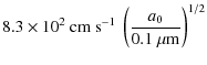
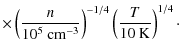
Thus, velocities between silicate dust particles are
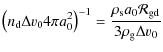
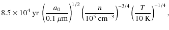
where
Equations (A.3) and (A.4) are only valid for solid particles. However, we can scale these relations to two arbitrary but equal aggregates of filling factor
![]() and (dimensionless) mass N. Because
and (dimensionless) mass N. Because
![]() and
and
![]() it follows that
it follows that
 |
(A.5b) |
where in the latter equation we substituted for simplicity the geometrical cross section
A.2 A simple analytical model for the initial stages of the growth
Despite the complexity of the recipe, it is instructive to approximate the initial collisional evolution of the dust size distribution with a simple analytical model (cf. Blum 2004). Figure 7 suggests that the initial evolution of
![]() can be divided in two regimes, where the transition point occurs at a mass N1. Initially (N<N1), the filling factor is in the fractal regime, which can be well approximated by a power-law,
can be divided in two regimes, where the transition point occurs at a mass N1. Initially (N<N1), the filling factor is in the fractal regime, which can be well approximated by a power-law,
![]() .
We refer to the fractal regime as including hit-and-stick collisions (no restructuring) as well as collisions for which
.
We refer to the fractal regime as including hit-and-stick collisions (no restructuring) as well as collisions for which
![]() but which do not lead to visible restructuring, i.e., only a small fraction of the grains take part in the restructuring. For N>N1 the filling factor starts to flatten-out. It is difficult to assign a trend for
but which do not lead to visible restructuring, i.e., only a small fraction of the grains take part in the restructuring. For N>N1 the filling factor starts to flatten-out. It is difficult to assign a trend for
![]() in the subsequent evolution. Following Fig. 7 we may assume that initially
in the subsequent evolution. Following Fig. 7 we may assume that initially
![]() stays approximately constant for several orders of magnitude in N, although at some point it will quickly assume its compact value of 33%. A sketch of the adopted porosity structure and the resulting scaling of velocities and timescales is presented in Fig. A.1, in which it is assumed that the collapse of the porous structure takes place after the point where the first erosive collisions occurs, at N=N2.
stays approximately constant for several orders of magnitude in N, although at some point it will quickly assume its compact value of 33%. A sketch of the adopted porosity structure and the resulting scaling of velocities and timescales is presented in Fig. A.1, in which it is assumed that the collapse of the porous structure takes place after the point where the first erosive collisions occurs, at N=N2.
![\begin{figure}
\par\includegraphics[width=80mm]{11158fA1}
\end{figure}](/articles/aa/full_html/2009/30/aa11158-08/img299.png) |
Figure A.1:
(gray solid line) A simplified model for the behavior of the filling factor with growth. Initially, for
|
| Open with DEXTER | |
From these expressions and the initial expressions for the relative velocity and the collision timescale (Eqs. (A.3) and (A.4)), the turn-over points N1 and N2 can be calculated. We assume that
![]() such that a fractal growth regime exist. Then, the first transition point is reached at a mass
such that a fractal growth regime exist. Then, the first transition point is reached at a mass
Unfortunately, the high powers make the numeric evaluation rather unstable. In our simulations we find that
![]() .
Subsequently, we can write for the second transition point, the onset of fragmentation, N2,
.
Subsequently, we can write for the second transition point, the onset of fragmentation, N2,


which corresponds also well to the results from the simulation for which
![\begin{figure}
\par\includegraphics[width=80mm]{11158fA2}
\end{figure}](/articles/aa/full_html/2009/30/aa11158-08/img314.png) |
Figure A.2:
Results of the simple analytic model (solid line) and comparison to the
|
| Open with DEXTER | |
 |
(A.7) |
where Eq. (A.4) is inserted for
see Fig. A.2, where we plotted the results of Eq. (A.8) together with the averaged mass and the mass-averaged mass of the distribution of the standard model. It follows that the fractal growth stages takes
Appendix B: The numerical collision experiments
The skeleton of our collision model consists of the outcomes of many aggregate-aggregate collision simulations. In this appendix we briefly review the setup of the simulations (Appendix B.1), discuss some auxiliary relations required to complete the collision model (Appendix B.2), discuss the output format of the binary collision model (Appendix B.3), and present a few limitations that arise due to our reliance on the outcomes of the numerical simulations (Appendix B.4).
B.1 Collision setup and input parameters
Collisions between aggregates are modeled using the soft aggregates numerical dynamics (SAND) code (Paszun & Dominik 2008; Dominik & Nübold 2002). This code treats interactions between individual grains held together by surface forces in a contact area (Derjaguin et al. 1975; Johnson et al. 1971). The SAND code calculates the equation of motion for each grain individually and simulates vibration, rolling, twisting, and sliding of the grains that are in contact. These interactions lead to energy dissipation via different channels. When two grains in contact are pulled away, the connection may break, causing loss of the energy. Monomers may also roll or slide over each other, through which energy is also dissipated (Dominik & Tielens 1997,1995,1996). For further details regarding this model and testing it against laboratory experiments we refer the reader to Paszun & Dominik (2008).
![\begin{figure}
\par\includegraphics[width=88mm]{11158fB1}
\end{figure}](/articles/aa/full_html/2009/30/aa11158-08/img322.png) |
Figure B.1:
Sketch of the initial setup of our simulations. The key input parameters |
| Open with DEXTER | |
Table B.1: Parameters used in the numerical simulations.
Relative velocities
The impact parameter b is also well sampled. We probe central collision (b=0), where aggregates can be compressed, grazing impacts (
![]() ), where particles can be stretched due to inertia, and several intermediate cases. In Table B.1 the impact parameter is defined relative to the outer radius of the particles,
), where particles can be stretched due to inertia, and several intermediate cases. In Table B.1 the impact parameter is defined relative to the outer radius of the particles,
![]() .
Here the outer radius
.
Here the outer radius
![]() is the radius of the smallest sphere centered at the center-of-mass of the particle that fully encloses it. In the Paszun & Dominik (2009) study the outcomes of a collision are averaged over the impact parameter b. However, in a Monte Carlo treatment, the averaging over impact is not necessary, and the normalized impact parameter
is the radius of the smallest sphere centered at the center-of-mass of the particle that fully encloses it. In the Paszun & Dominik (2009) study the outcomes of a collision are averaged over the impact parameter b. However, in a Monte Carlo treatment, the averaging over impact is not necessary, and the normalized impact parameter
![]() can be determined using a random deviate
can be determined using a random deviate
![]() ,
i.e.,
,
i.e.,
![]() .
We have chosen to use the raw data sampled by the Paszun & Dominik (2009) parameter study, explicitly including
.
We have chosen to use the raw data sampled by the Paszun & Dominik (2009) parameter study, explicitly including ![]() as an input parameter for the Monte Carlo model. In this way the effects of off-center impacts can be assessed, i.e., by comparing it to models that contain only head-on collisions.
as an input parameter for the Monte Carlo model. In this way the effects of off-center impacts can be assessed, i.e., by comparing it to models that contain only head-on collisions.
The internal structure of the aggregates, or initial compactness, is characterized by the geometrical filling factor,
![]() (Eq. (7)). To obtain
(Eq. (7)). To obtain
![]() ,
the projected surface area,
,
the projected surface area, ![]() ,
is averaged over a large number of different orientations of the particle. The parameter space of the filling factor
,
is averaged over a large number of different orientations of the particle. The parameter space of the filling factor
![]() is chosen such that we sample very porous, fractal aggregates that grow due to the Brownian motion (Paszun & Dominik 2006; Blum & Schräpler 2004), through intermediate compactness aggregates that form by particle-cluster aggregation (PCA), up to compact aggregates that may result from collisional compaction.
is chosen such that we sample very porous, fractal aggregates that grow due to the Brownian motion (Paszun & Dominik 2006; Blum & Schräpler 2004), through intermediate compactness aggregates that form by particle-cluster aggregation (PCA), up to compact aggregates that may result from collisional compaction.
The final parameter that determines a collision outcome is the mass ratio, N2/N1 (N1 being the larger aggregate). The Paszun & Dominik (2009) experiments sample a mass ratio between 1 and 10-3. In this study, however, we will only use the collisions corresponding to the two extreme values (i.e., mass ratios of 1 and 10-3) as representatives of two distinct classes: global and local.
B.2 Auxiliary relations for the collision recipe
There are a few more relations required for a consistent approach to the collision recipe. These are presented here for completeness.B.2.1 The filling factor of small fragments
A common filling factor can be assigned to the small fragments produced by erosive or fragmenting collisions that constitute the power-law component. The compactness of these particles depends only on mass and is presented in Fig. B.2, where fragments produced in many simulations, reflecting a variety of collision properties, are plotted. Almost all particles are located along the power-law with the slope of -0.33. This provides an easy prescription for the filling factor of small fragments. The dependence indicates a fractal structure (with the fractal dimension of about
![]() )
of aggregates formed in a fragmentation event, since non-fractal aggregates would have a filling factor independent of mass.
)
of aggregates formed in a fragmentation event, since non-fractal aggregates would have a filling factor independent of mass.
![\begin{figure}
\par\includegraphics[width=88mm,clip]{11158fB2}
\end{figure}](/articles/aa/full_html/2009/30/aa11158-08/img334.png) |
Figure B.1:
The geometrical filling factor as a function of fragment mass. Many simulations with different sets of parameters are overplotted. The dashed line indicates the least square power-law fit,
|
| Open with DEXTER | |
As shown by Paszun & Dominik (2009), after reaching the maximum compaction, further increase of the impact energy produces more restructuring and results in a flattening of the produced aggregate. Therefore, very fluffy particles can be produced in collisions of massive aggregates, where the power-law component extends to larger N. This behavior is also observed in Fig. B.2, where fluffy, small fragments follow the power-law relation, while some large, still compact particles are above the dashed line.
B.2.2 Relation between a
 and a
and a
In this study we characterize aggregates by two different radii: the outer radius
![]() and the projected surface equivalent radius
and the projected surface equivalent radius ![]() .
The first is used as a reference to the impact parameter b, i.e., the collision offset is determined relative to the largest impact parameter,
.
The first is used as a reference to the impact parameter b, i.e., the collision offset is determined relative to the largest impact parameter,
![]() .
The cross-section equivalent radius
.
The cross-section equivalent radius ![]() defines our structural parameter
defines our structural parameter
![]() (see Eq. (7)). We determine the relation between the two radii (
(see Eq. (7)). We determine the relation between the two radii (
![]() and
and ![]() )
empirically. Both
)
empirically. Both
![]() and
and ![]() are determined for many aggregates of various shape and mass. We sample particles with the fractal dimension in the range of
are determined for many aggregates of various shape and mass. We sample particles with the fractal dimension in the range of
![]() and masses from several to a few thousands monomer masses. These aggregates were produced using an algorithm developed by Filippov et al. (2000).
and masses from several to a few thousands monomer masses. These aggregates were produced using an algorithm developed by Filippov et al. (2000).
![\begin{figure}
\par\includegraphics[width=88mm,clip]{11158fB3}
\end{figure}](/articles/aa/full_html/2009/30/aa11158-08/img336.png) |
Figure B.2:
The geometrical filling factor dependence on the ratio of outer to geometrical radii. In this figure we plot
|
| Open with DEXTER | |
In order to provide a simple relation between the two radii, two power-law functions are fitted to the two regimes: compact particles below
![]() and fluffy aggregates above that limit. These two functions are given by
and fluffy aggregates above that limit. These two functions are given by
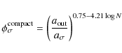
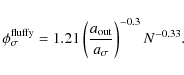
To further verify these relations we use particles produced in several simulations performed by Paszun & Dominik (2009). These aggregates are indicated in Fig. B.3 by black squares. They show a similar relation to the one obtained in Eq. (B.1). Points that are slightly shifted above the fitted lines correspond to aggregates that are partly compressed (they did not reach the maximum compaction). Their compact cores are still surrounded by a fluffy exterior that causes a small increase of the ratio of the outer radius over the projected surface equivalent radius
We remark here that, although the fits present a general picture, situations where
![]() are not likely to materialize when
are not likely to materialize when ![]() .
This would corresponds to very open fractals of fractal dimension less than two. Instead, in our models
.
This would corresponds to very open fractals of fractal dimension less than two. Instead, in our models
![]() and we therefore always have
and we therefore always have
![]() .
Consequently, the fraction of missing collisions
.
Consequently, the fraction of missing collisions
![]() is close to zero in most of the cases.
is close to zero in most of the cases.
B.2.3 Hit and stick
At very low energies (
![]() )
two aggregates will stick where they meet, without affecting the internal structure of the particles. This is the ``hit-and-stick'' regime in which the collisional growth can often be described by fractal laws. Two important limits are cluster-cluster coagulation (CCA) and particle-cluster coagulation (PCA). In the former, two particles of equal size meet, which often results in very fluffy structures, whereas PCA describes the process in which the projectile particles are small with respect to the target. The filling factor then saturates to a constant value. In the case of monomers, the filling factor will reach
)
two aggregates will stick where they meet, without affecting the internal structure of the particles. This is the ``hit-and-stick'' regime in which the collisional growth can often be described by fractal laws. Two important limits are cluster-cluster coagulation (CCA) and particle-cluster coagulation (PCA). In the former, two particles of equal size meet, which often results in very fluffy structures, whereas PCA describes the process in which the projectile particles are small with respect to the target. The filling factor then saturates to a constant value. In the case of monomers, the filling factor will reach ![]() (Kozasa et al. 1992).
(Kozasa et al. 1992).
In general particles do not merely collide with either similar-size particles or monomers. Every size-ratio is possible and leads to a different change in filling factor. Ormel et al. (2007) provide an analytical expression, based upon fits to collision experiments of Ossenkopf (1993), that give the increase in void space as function of the geometrical volume of the collision partners. Here, the geometrical volume V is the volume that corresponds to the geometrical radius, ![]() .
In this study additional numerical collision experiments were used to further constrain these analytical fits. These experiments involved several ``monomer-bombardments'' of aggregates of different initial filling factor. Using these data, we fit the volume increase as
.
In this study additional numerical collision experiments were used to further constrain these analytical fits. These experiments involved several ``monomer-bombardments'' of aggregates of different initial filling factor. Using these data, we fit the volume increase as
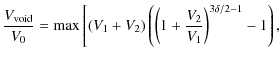
![$\displaystyle \left. \frac{N_2}{0.087\phi_2} \qquad \exp\left[-\left(\frac{15V_2}{V_1}\right)^{0.25}\right] \right] ,$](/articles/aa/full_html/2009/30/aa11158-08/img349.png)
where
![]() is the increase in void space (leading to a lower
is the increase in void space (leading to a lower
![]() ), V1>V2 the geometrical volumes of the collision partner, N2 the number of grains in the smaller particle, and V0 the monomer volume. The first term converges to CCA in the limit of V2=V1, and is the same as in Ormel et al. (2007). Here,
), V1>V2 the geometrical volumes of the collision partner, N2 the number of grains in the smaller particle, and V0 the monomer volume. The first term converges to CCA in the limit of V2=V1, and is the same as in Ormel et al. (2007). Here,
![]() is an exponent that reflects the fractal growth in this limit (Ossenkopf 1993). The second expression converges to PCA in the limit of
is an exponent that reflects the fractal growth in this limit (Ossenkopf 1993). The second expression converges to PCA in the limit of
![]() .
The rationale of providing a second expression is that in the case of
.
The rationale of providing a second expression is that in the case of
![]() (PCA) the first expression goes to zero very quickly (no voids are added), which is inconsistent with the PCA limit of 15%. From the results of our new collision experiments we have introduced an exponent of 0.25 to the PCA-part of Eq. (B.2), which softens the decrease of
(PCA) the first expression goes to zero very quickly (no voids are added), which is inconsistent with the PCA limit of 15%. From the results of our new collision experiments we have introduced an exponent of 0.25 to the PCA-part of Eq. (B.2), which softens the decrease of
![]() with increasing mass ratio.
with increasing mass ratio.
However, not all numerical experiments could be fitted equally well. In fact, we had to compromise. It is likely that a better fit involves more parameters, e.g., the elongation of the aggregates or their fractal dimension. Here, we have adopted approximate fits that follow the qualitative picture in both the CCA (V1 = V2) and the PCA (
![]() )
limit. Remark, finally, that for the molecular cloud environment the hit-and-stick regime is only relevant in the initial stages of coagulation at densities of
)
limit. Remark, finally, that for the molecular cloud environment the hit-and-stick regime is only relevant in the initial stages of coagulation at densities of
![]() or grain sizes
or grain sizes
![]() .
.
B.3 The collision tables
Given the level of complexity, it is not feasible to provide simple analytical expressions for the collision outcome (in terms of the parameters listed in Table 1) as function of the collision parameters (
Each table lists one output quantity as function of the dimensionless energy parameter
![]() and the initial filling factor of aggregates
and the initial filling factor of aggregates
![]() .
The only exception concerns the fraction of missed collisions,
.
The only exception concerns the fraction of missed collisions,
![]() .
This quantity provides a correction to the collision cross-section of particles, in our case calculated from the outer radius of an aggregate
.
This quantity provides a correction to the collision cross-section of particles, in our case calculated from the outer radius of an aggregate
![]() (cf. Appendix C). The filling factor
(cf. Appendix C). The filling factor
![]() is not an appropriate quantity to use here, because it is ambiguous where it concerns the structure of particles. For example, low
is not an appropriate quantity to use here, because it is ambiguous where it concerns the structure of particles. For example, low
![]() could mean either a very fractal structure (and correspondingly high number of missing collisions) or a porous but homogeneous structure (and low number of missing collisions). Therefore, it is more appropriate to relate the probability of a collision miss to the radii with which the particle is characterized. Thus,
could mean either a very fractal structure (and correspondingly high number of missing collisions) or a porous but homogeneous structure (and low number of missing collisions). Therefore, it is more appropriate to relate the probability of a collision miss to the radii with which the particle is characterized. Thus,
![]() is provided as a function of the ratio of the outer radius over the projected surface equivalent radius,
is provided as a function of the ratio of the outer radius over the projected surface equivalent radius,
![]() .
.
Table B.1:
Example of an output table from the online data (
![]() at b=0 in the global recipe).
at b=0 in the global recipe).
# GLOBAL, b=0.0, Q=fpwlTherefore, Table B.2 presents the fraction of mass in the power-law component,
In each table the first column and the first row specify the normalized energy parameter
![]() and the initial filling factor
and the initial filling factor
![]() (or the ratio of the outer over the geometrical radii
(or the ratio of the outer over the geometrical radii
![]() in the case of
in the case of
![]() ), respectively. Here,
), respectively. Here,
![]() denotes the collision energy scaled by a normalization constant that involves (i) the breaking or rolling energy and (ii) the reduced or total number of particles, see Sect. 3.2 and Table 1. In the case of Table B.2 the scaling parameter is
denotes the collision energy scaled by a normalization constant that involves (i) the breaking or rolling energy and (ii) the reduced or total number of particles, see Sect. 3.2 and Table 1. In the case of Table B.2 the scaling parameter is
![]() .
.
Table B.3 is the second example. It is taken from the local recipe and it presents the
![]() quantity for the head-on collision. The dimensionless energy parameter
quantity for the head-on collision. The dimensionless energy parameter
![]() has fewer entries in the local recipe tables than in the global recipe. In Table B.3 the energy is scaled by reduced number of monomers
has fewer entries in the local recipe tables than in the global recipe. In Table B.3 the energy is scaled by reduced number of monomers ![]() (local recipe scaling) and by the breaking energy
(local recipe scaling) and by the breaking energy
![]() (erosion scaling) as indicated in Table 1. The header in this case is
(erosion scaling) as indicated in Table 1. The header in this case is
# LOCAL, b=0.0, Q=fpwlNote that in the local recipe the filling factors are lower. In this case larger aggregates are used to model collisions at large mass ratio, N1/N2 = 103. The fractal structure of these aggregates results in a lower filling factor.
B.4 Limitations of the collision recipe
The main limitation of the collision recipe is that, due to computational constraints, the binary aggregate simulations can only simulate aggregates of a mass ![]() .
For the recipe to become applicable for large aggregates scaling of the results of the collision experiments is required. This is a critical point of the recipe for which suitable dimensionless quantities had to be determined.
However, the extrapolation assumes that the collision physics that determines the outcomes of collisions at low-N also holds at large scales. This is a crucial assumption in which collisional outcomes like bouncing are a priori not possible because these do not take place at the low-N part of the simulations.
.
For the recipe to become applicable for large aggregates scaling of the results of the collision experiments is required. This is a critical point of the recipe for which suitable dimensionless quantities had to be determined.
However, the extrapolation assumes that the collision physics that determines the outcomes of collisions at low-N also holds at large scales. This is a crucial assumption in which collisional outcomes like bouncing are a priori not possible because these do not take place at the low-N part of the simulations.
Table 6:
Example of an output table from the online data (
![]() at b=0 in the local recipe).
at b=0 in the local recipe).
Bouncing of aggregates is observed in laboratory experiments (Blum & Münch 1993; Weidling et al. 2009; Blum 2006; Langkowski et al. 2008), whereas it does not occur in our simulations. For silicates, bouncing occurs at sizes above approximately ![]() m (i.e., N>109 particles) and is not fully understood from a microphysical perspective. In the case of ice-coated silicate grains, which provide stronger adhesion forces, our simulations show that growth proceeds to
m (i.e., N>109 particles) and is not fully understood from a microphysical perspective. In the case of ice-coated silicate grains, which provide stronger adhesion forces, our simulations show that growth proceeds to ![]()
![]() sizes. In this case, therefore, bouncing might slow down the growth earlier than observed in our experiments, especially when the internal structure has already re-adjusted to a compact state. However, it is presently unclear how these laboratory experiments apply to ice aggregates and hence whether and to what extent the results would be affected by bouncing. We recognize that this may, potentially, present a limitation to the growth of aggregates in molecular clouds, but also emphasize it will not affect the main conclusions from this study as in only a few models aggregates grow to sizes
sizes. In this case, therefore, bouncing might slow down the growth earlier than observed in our experiments, especially when the internal structure has already re-adjusted to a compact state. However, it is presently unclear how these laboratory experiments apply to ice aggregates and hence whether and to what extent the results would be affected by bouncing. We recognize that this may, potentially, present a limitation to the growth of aggregates in molecular clouds, but also emphasize it will not affect the main conclusions from this study as in only a few models aggregates grow to sizes ![]() 100
100
![]() .
.
Another assumption of the collision model is that the grains have a spherical geometry. Again, computational constraints rule out numerical modeling of randomly shaped particles. Whether erratically shaped grains would help or harm the sticking or bouncing is unclear. Because the strength of an aggregate is determined by the amount of contact area between two grains, the strength of irregularly shaped monomers depends on the local radius of curvature. Therefore, highly irregular grains are held by contacts of much smaller size, because they are connected by surface asperities. On the other hand, irregular grains may form more than one contact. However, the geometry of the grains does not necessarily pose a bottleneck to the validity of the collision model. Instead, like the size distribution, the consequence of irregularly shaped monomers is reflected in a different energy scaling.
Appendix C: The Monte Carlo program
The advantage of a Monte Carlo (MC) approach to the calculation of the collisional evolution is that collisions are modeled individually and that they, therefore, bear a direct correspondence to the collision model. Furthermore, in a MC approach structural parameters (like
By virtue of the scaling relations discussed in Sect. 3.2 the MC coagulation model is able to treat much larger aggregates than the binary collision experiments. A broad size distributions, which may, e.g., result from injection of small particles due to fragmentation, can, however, become problematic for a MC approach, since the high dynamic range required consumes computational resources. To overcome this problem we use the grouping method outlined by Ormel & Spaans (2008). In this method the 1-1 correspondence between a simulation particle and a physical particle is dropped; instead, the simulated particles are represented by groups of identical physical particles. The group's mass is determined by the peak of the m2f(m) mass distribution - denoted ![]() - and particles of smaller mass ``travel'' together in groups of total mass
- and particles of smaller mass ``travel'' together in groups of total mass ![]() .
Grouping entails that a large particle can collide with many small particles simultaneously - a necessary approximation of the collision process.
.
Grouping entails that a large particle can collide with many small particles simultaneously - a necessary approximation of the collision process.
Below, we present the way in which we have implemented the collision recipe with the grouping method of Ormel & Spaans (2008).
C.1 Collision rates
The cycle starts with the calculation (or update) of the collision rates between the groups of the simulation. The individual collision rate between two particles i and j is
C.2 Determination of collision partners
Random numbers determine which two groups collide and the number of particles that are involved from the i and j groups,
![\begin{figure}
\par\includegraphics[width=88mm,clip]{11158fC1}
\end{figure}](/articles/aa/full_html/2009/30/aa11158-08/img375.png) |
Figure C.1:
Illustration of the picking of the grid points. The collision takes place at
|
| Open with DEXTER | |
C.3 Determining the collision quantities in grouped collisions
When the collision is in the ``hit-and-stick'' regime the properties of the new particles are easily found by adding the masses of the j-particles to the i-particle and calculating their filling factor using Eq. (B.2). We therefore concentrate here on the local or global recipe. The collision is then characterized by the three dimensionless parameters: normalized collision energy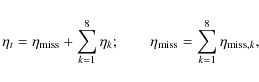 |
(C.1) |
where
We continue with the general case of multiple occupied grid points. First, we consider the mass that is eroded, given by the
![]() quantities. The mass eroded at one grid point per collision is given by
quantities. The mass eroded at one grid point per collision is given by
![]() (global recipe) or
(global recipe) or
![]() (local recipe). Then, the total mass eroded by the group collision is
(local recipe). Then, the total mass eroded by the group collision is
 |
(C.2) |
If this quantity is more than mi, clearly there is no large fragment component
where P2,k is the probability that breakage occurs at a grid point and follows from the
The last quantity to determine is the change in the filling factor of the large aggregate, denoted by the ![]() symbol for one collision. Like Eq. (C.3) we multiply the changes in
symbol for one collision. Like Eq. (C.3) we multiply the changes in ![]() at the individual grid nodes,
at the individual grid nodes,
This completes the implementation of the collisional outcome within the framework of the grouping mechanism. That is, we have the masses and the filling factor of the large fragment component (
C.4 Picking of the power-law component masses
The final part of the MC cycle is to pick particles according to the power-law distribution, under the constraints of a total mass![\begin{displaymath}m_{\rm small} = m_0\left[1 + \overline{r}\left( \left(\frac{m_{\rm rem}}{m_0}\right)^{1+q} -1\right)\right]^{1/(1+q)},
\end{displaymath}](/articles/aa/full_html/2009/30/aa11158-08/img399.png)
where
C.5 Merging/Duplication
The final part of the MC program consist of an inventory, and possible adjustment, of the amount of groups and species (
Appendix D: List of symbols
| Symbol | Description |
|
|
Reduced modulus of elasticity (Eq. (9)) |
|
|
Gas-to-dust ratio by mass |
| Relative velocity (Appendix A) | |
| Surface energy density (Eq. (9)) | |
| Number of particles or groups (Appendix C) | |
|
|
Geometrical filling factor (Eq. (7)) |
| Molecular mass (Sect. 2) | |
|
|
Molecular, turbulent viscosity (Sect. 2.1) |
|
|
Critical displacement for irreversible rolling (Eq. (9)) |
|
|
Material density,
|
|
|
Gas density,
|
| Average projected surface area (Sect. 3) | |
|
|
Collisional cross section (Sect. 3) |
|
|
Friction time (Eq. (A.1)) |
| Change in geometrical filling factor, | |
|
|
|
| Fractal dimension | |
| E | Collision energy,
|
|
|
Rolling energy (Eq. (9)) |
|
|
Breaking energy (Eq. (9)) |
| N | Number of grains in aggregate (dimensionless |
| measure of mass) | |
| Reduced number of monomers in collision | |
|
|
|
| Number of big fragments | |
|
|
Total number of monomers in collision,
|
| Reynolds number (Eq. (5)) | |
| Spread in number of fragments of big component (Sect. 3.3) | |
| St | Particle Stokes number (Appendix A) |
| T | Temperature (Sect. 2.1) |
| a0 | Monomer radius |
|
|
Aggregate outer radius (Fig. 1) |
| Aggregate geometrical radius (projected surface | |
| equivalent radius) (Fig. 1) | |
| Reduced radius (Eq. (9)) | |
| b | Impact parameter |
|
|
Sum of the outer radii,
|
| Normalized impact parameter,
|
|
| Sound speed (gas) | |
|
|
Fraction of collision misses (Sect. 3.3) |
|
|
Fraction of mass in power-law component (Sect. 3.3) |
| n | Particle density (gas) |
| m | Particle mass |
| Reduced mass | |
| Hydrogen mass | |
| q | Power-law exponent (size distribution) (Sect. 3.3) |
|
|
Random deviate |
|
|
Ambipolar diffusion time (Eq. (2)) |
|
|
Initial collision time (Eq. (A.4)) |
|
|
Free-fall time (Eq. (1)) |
| Inner (Kolmogorov) eddy turn-over time (Eq. (6)) | |
| Large eddy turn-over velocity (Sect. 2.1) | |
| Inner (Kolmogorov) eddy turn-over velocity (Eq. (6)) |
References
- Aikawa, Y., Wakelam, V., Garrod, R. T., & Herbst, E. 2008, ApJ, 674, 984 [NASA ADS] [CrossRef]
- Akyilmaz, M., Flower, D. R., Hily-Blant, P., Pineau Des Forêts, G., & Walmsley, C. M. 2007, A&A, 462, 221 [NASA ADS] [CrossRef] [EDP Sciences]
- Alves, J., Lombardi, M., & Lada, C. J. 2007, A&A, 462, L17 [NASA ADS] [CrossRef] [EDP Sciences]
- Bergin, E. A., & Tafalla, M. 2007, ARA&A, 45, 339 [NASA ADS] [CrossRef]
- Binney, J., & Tremaine, S. 1987, Galactic dynamics (Princeton, NJ: Princeton University Press), 747 (In the text)
- Blum, J. 2004, in Astrophysics of Dust, ed. A. N. Witt, G. C. Clayton, & B. T. Draine, ASP Conf. Ser., 309, 369 (In the text)
- Blum, J. 2006, Adv. Phys., 55, 881 [NASA ADS] [CrossRef]
- Blum, J., & Münch, M. 1993, Icarus, 106, 151 [NASA ADS] [CrossRef]
- Blum, J., & Schräpler, R. 2004, Phys. Rev. Lett., 93, 115503 [NASA ADS] [CrossRef] (In the text)
- Blum, J., & Wurm, G. 2000, Icarus, 143, 138 [NASA ADS] [CrossRef] (In the text)
- Blum, J., & Wurm, G. 2008, ARA&A, 46, 21 [NASA ADS] [CrossRef]
- Blum, J., Schräpler, R., Davidsson, B. J. R., & Trigo-Rodríguez, J. M. 2006, ApJ, 652, 1768 [NASA ADS] [CrossRef]
- Bowey, J. E., Adamson, A. J., & Whittet, D. C. B. 1998, MNRAS, 298, 131 [NASA ADS] [CrossRef]
- Brauer, F., Dullemond, C. P., & Henning, T. 2008, A&A, 480, 859 [NASA ADS] [CrossRef] [EDP Sciences] (In the text)
- Butler, M. J., & Tan, J. C. 2009, ApJ, 696, 484 [NASA ADS] [CrossRef] (In the text)
- Carrasco, L., Strom, S. E., & Strom, K. M. 1973, ApJ, 182, 95 [NASA ADS] [CrossRef]
- Charnley, S. B., Tielens, A. G. G. M., & Millar, T. J. 1992, ApJ, 399, L71 [NASA ADS] [CrossRef]
- Chiar, J. E., Ennico, K., Pendleton, Y. J., et al. 2007, ApJ, 666, L73 [NASA ADS] [CrossRef] (In the text)
- Chokshi, A., Tielens, A. G. G. M., & Hollenbach, D. 1993, ApJ, 407, 806 [NASA ADS] [CrossRef]
- Derjaguin, B. V., Muller, V. M., & Toporov, Y. P. 1975, J. Coll. Interf. Sci., 53, 314 [CrossRef]
- Desert, F.-X., Boulanger, F., & Puget, J. L. 1990, A&A, 237, 215 [NASA ADS]
- Dominik, C., & Nübold, H. 2002, Icarus, 157, 173 [NASA ADS] [CrossRef]
- Dominik, C., & Tielens, A. G. G. M. 1995, Philosoph. Mag. A, 72, 783 [NASA ADS] [CrossRef]
- Dominik, C., & Tielens, A. G. G. M. 1996, Philosoph. Mag. A, 73, 1279 [NASA ADS] [CrossRef]
- Dominik, C., & Tielens, A. G. G. M. 1997, ApJ, 480, 647 [NASA ADS] [CrossRef]
- Draine, B. T. 1985, in Protostars and Planets II, ed. D. C. Black, & M. S. Matthews, 621 (In the text)
- Draine, B. T., & Lee, H. M. 1984, ApJ, 285, 89 [NASA ADS] [CrossRef] (In the text)
- Filippov, A., Zurita, M., & Rosner, D. 2000, J. Coll. Interf. Sci., 229, 261 [CrossRef] (In the text)
- Flower, D. R., Pineau Des Forêts, G., & Walmsley, C. M. 2006, A&A, 456, 215 [NASA ADS] [CrossRef] [EDP Sciences]
- Goldsmith, P. F., Bergin, E. A., & Lis, D. C. 1997, ApJ, 491, 615 [NASA ADS] [CrossRef] (In the text)
- Hartmann, L., Ballesteros-Paredes, J., & Bergin, E. A. 2001, ApJ, 562, 852 [NASA ADS] [CrossRef] (In the text)
- Hasegawa, T. I., Herbst, E., & Leung, C. M. 1992, ApJS, 82, 167 [NASA ADS] [CrossRef]
- Hirashita, H., & Yan, H. 2009, MNRAS, 394, 1061 [NASA ADS] [CrossRef]
- Huss, G. R., MacPherson, G. J., Wasserburg, G. J., Russell, S. S., & Srinivasan, G. 2001, Meteo. Planet. Sci., 36, 975 [NASA ADS] (In the text)
- Johnson, K. L., Kendall, K., & Roberts, A. D. 1971, Proc. Royal Soc. A, 324, 301 [NASA ADS] [CrossRef]
- Johnstone, D., & Bally, J. 2006, ApJ, 653, 383 [NASA ADS] [CrossRef]
- Jones, A. P., Tielens, A. G. G. M., & Hollenbach, D. J. 1996, ApJ, 469, 740 [NASA ADS] [CrossRef]
- Jørgensen, J. K., Johnstone, D., Kirk, H., et al. 2008, ApJ, 683, 822 [NASA ADS] [CrossRef]
- Jura, M. 1980, ApJ, 235, 63 [NASA ADS] [CrossRef] (In the text)
- Kawamura, A., Onishi, T., Yonekura, Y., et al. 1998, ApJS, 117, 387 [NASA ADS] [CrossRef] (In the text)
- Klessen, R. S., Ballesteros-Paredes, J., Vázquez-Semadeni, E., & Durán-Rojas, C. 2005, ApJ, 620, 786 [NASA ADS] [CrossRef]
- Kozasa, T., Blum, J., & Mukai, T. 1992, A&A, 263, 423 [NASA ADS] (In the text)
- Langkowski, D., Teiser, J., & Blum, J. 2008, ApJ, 675, 764 [NASA ADS] [CrossRef]
- Mac Low, M.-M., & Klessen, R. S. 2004, Rev. Mod. Phys., 76, 125 [NASA ADS] [CrossRef]
- Markiewicz, W. J., Mizuno, H., & Völk, H. J. 1991, A&A, 242, 286 [NASA ADS] (In the text)
- Mathis, J. S., Rumpl, W., & Nordsieck, K. H. 1977, ApJ, 217, 425 [NASA ADS] [CrossRef] (In the text)
- McClure, M. 2009, ApJ, 693, L81 [NASA ADS] [CrossRef] (In the text)
- Meakin, P. 1988, Ann. Rev. Phys. Chem., 39, 237 [CrossRef]
- Meakin, P., & Donn, B. 1988, ApJ, 329, L39 [NASA ADS] [CrossRef]
- Min, M., Hovenier, J. W., Waters, L. B. F. M., & de Koter, A. 2008, A&A, 489, 135 [NASA ADS] [CrossRef] [EDP Sciences]
- Ormel, C. W., & Cuzzi, J. N. 2007, A&A, 466, 413 [NASA ADS] [CrossRef] [EDP Sciences] (In the text)
- Ormel, C. W., & Spaans, M. 2008, ApJ, 684, 1291 [NASA ADS] [CrossRef] (In the text)
- Ormel, C. W., Spaans, M., & Tielens, A. G. G. M. 2007, A&A, 461, 215 [NASA ADS] [CrossRef] [EDP Sciences]
- Ossenkopf, V. 1993, A&A, 280, 617 [NASA ADS] (In the text)
- Paszun, D., & Dominik, C. 2006, Icarus, 182, 274 [NASA ADS] [CrossRef]
- Paszun, D., & Dominik, C. 2008, A&A, 484, 859 [NASA ADS] [CrossRef] [EDP Sciences]
- Paszun, D., & Dominik, C. 2009, A&A, submitted
- Schnee, S., Li, J., Goodman, A. A., & Sargent, A. I. 2008, ApJ, 684, 1228 [NASA ADS] [CrossRef] (In the text)
- Shen, Y., Draine, B. T., & Johnson, E. T. 2008, ApJ, 689, 260 [NASA ADS] [CrossRef]
- Shu, F. H. 1977, ApJ, 214, 488 [NASA ADS] [CrossRef] (In the text)
- Stepnik, B., Abergel, A., Bernard, J.-P., et al. 2003, A&A, 398, 551 [NASA ADS] [CrossRef] [EDP Sciences] (In the text)
- Suyama, T., Wada, K., & Tanaka, H. 2008, ApJ, 684, 1310 [NASA ADS] [CrossRef]
- Tassis, K., & Mouschovias, T. C. 2004, ApJ, 616, 283 [NASA ADS] [CrossRef] (In the text)
- Tielens, A. G. G. M. 2005, The Physics and Chemistry of the Interstellar Medium, The Physics and Chemistry of the Interstellar Medium, ed. A. G. G. M. Tielens (Cambridge, UK: Cambridge University Press) (In the text)
- Tielens, A. G. G. M., & Hagen, W. 1982, A&A, 114, 245 [NASA ADS]
- van Breemen, J. M., Min, M., Chiar, J. E., et al. 2009, A&A submitted
- Völk, H. J., Morfill, G. E., Roeser, S., & Jones, F. C. 1980, A&A, 85, 316 [NASA ADS] (In the text)
- Wada, K., Tanaka, H., Suyama, T., Kimura, H., & Yamamoto, T. 2008, ApJ, 677, 1296 [NASA ADS] [CrossRef]
- Weidenschilling, S. J., & Cuzzi, J. N. 1993, in Protostars and Planets III, ed. E. H. Levy, & J. I. Lunine, 1031 (In the text)
- Weidenschilling, S. J., & Ruzmaikina, T. V. 1994, ApJ, 430, 713 [NASA ADS] [CrossRef] (In the text)
- Weidling, R., Güttler, C., Blum, J., & Brauer, F. 2009, ApJ, 694, 2036 [NASA ADS] [CrossRef]
- Weingartner, J. C., & Draine, B. T. 2001, ApJ, 548, 296 [NASA ADS] [CrossRef]
- Whittet, D. C. B. 2005, in Astronomical Polarimetry: Current Status and Future Directions, ed. A. Adamson, C. Aspin, C. Davis, & T. Fujiyoshi, ASP Conf. Ser., 343, 321
- Wilking, B. A., Lebofsky, M. J., Kemp, J. C., Martin, P. G., & Rieke, G. H. 1980, ApJ, 235, 905 [NASA ADS] [CrossRef]
- Winston, E., Megeath, S. T., Wolk, S. J., et al. 2007, ApJ, 669, 493 [NASA ADS] [CrossRef] (In the text)
- Wood, J. A. 1998, ApJ, 503, L101 [NASA ADS] [CrossRef] (In the text)
- Yan, H., Lazarian, A., & Draine, B. T. 2004, ApJ, 616, 895 [NASA ADS] [CrossRef] (In the text)
- Zsom, A., & Dullemond, C. P. 2008, A&A, 489, 931 [NASA ADS] [CrossRef] [EDP Sciences]
Footnotes
- ... clouds
- Collision tables are only available in electronic form at the CDS via anonymous ftp to cdsarc.u-strasbg.fr (130.79.128.5) or via http://cdsweb.u-strasbg.fr/cgi-bin/qcat?J/A+A/502/845
- ... radius
- A list of symbols is provided in Appendix D.
- ... gas
- Note that our definition of density - n, the number of gas molecules per cm3 - differs from the density of hydrogen nuclei (
 ), which is more commonly referred to as density in the dust/ISM communities. For cosmic abundances
is related to n as
), which is more commonly referred to as density in the dust/ISM communities. For cosmic abundances
is related to n as
 .
.
- ... aggregates
- The compactness parameter
is the inverse of the enlargement factor
 ,
previously used in Ormel et al. (2007). Ossenkopf (1993) uses
,
previously used in Ormel et al. (2007). Ossenkopf (1993) uses
 as its structural parameter.
- ... tables
- The tables are provided online.
- ... component
- Recall that in grouped collisions (
 )
this implies that the grouping method is not fully accurate as the change in mass is of the order of the mass itself; but the procedure is always fine if
)
this implies that the grouping method is not fully accurate as the change in mass is of the order of the mass itself; but the procedure is always fine if
 .
.
All Tables
Table 1: Quantities provided by the adjusted collision recipe.
Table 2: List of the model runs.
Table 3:
Mass-weighted size of the distribution,
![]() ,
at several distinct events during the simulation run.
,
at several distinct events during the simulation run.
Table 4:
Like Table 3 but for the geometrical opacity ![]() of the particles.
of the particles.
Table B.1: Parameters used in the numerical simulations.
Table B.1:
Example of an output table from the online data (
![]() at b=0 in the global recipe).
at b=0 in the global recipe).
Table 6:
Example of an output table from the online data (
![]() at b=0 in the local recipe).
at b=0 in the local recipe).
All Figures
| |
Figure 1:
2D projection of a fluffy aggregate with indication of the geometrical radii, |
| Open with DEXTER | |
| In the text | |
| |
Figure 2: Schematic decision chain employed to distinguish between the hit-and-stick, global, and local recipes. |
| Open with DEXTER | |
| In the text | |
| |
Figure 3:
Sketch of the adopted formalism for the size distribution with which the results of the aggregate collision simulation are quantified. See text and Table 1 for the description of the symbols. If
|
| Open with DEXTER | |
| In the text | |
| |
Figure 4:
Quantities provided by the local recipe.
The left panel shows the mass in small fragments of the power-law component, normalized to the reduced mass of the colliding aggregates
|
| Open with DEXTER | |
| In the text | |
| |
Figure 5:
Quantities provided by the global recipe.
Left panels correspond to central collisions, while the right panels correspond to off-center collisions at normalized impact parameter
|
| Open with DEXTER | |
| In the text | |
| |
Figure 6:
Mass distribution of the standard model (
|
| Open with DEXTER | |
| In the text | |
| |
Figure 7:
The distribution of the filling factor,
|
| Open with DEXTER | |
| In the text | |
| |
Figure 8:
(solid curves) The mean size
|
| Open with DEXTER | |
| In the text | |
| |
Figure 9:
The effects of the collision recipe on the evolution of the size distribution. The standard model (b, shown for comparison) is varied and features: (a) compact coagulation, in which the filling factor is restricted to a lower limit of 33%; (c) head-on collisions only, where the impact parameter is fixed at b=0 for every collision. The calculations last for
|
| Open with DEXTER | |
| In the text | |
| |
Figure 10:
Distribution plots corresponding to the collisional evolution of silicates (left panels) and ice-coated silicates
(right panels) at densities of
n=104, 105 and
|
| Open with DEXTER | |
| In the text | |
| |
Figure 11:
The effects of a different grain size a0 to the collisional evolution: (a)
|
| Open with DEXTER | |
| In the text | |
| |
Figure 12:
The opacity |
| Open with DEXTER | |
| In the text | |
| |
Figure A.1:
(gray solid line) A simplified model for the behavior of the filling factor with growth. Initially, for
|
| Open with DEXTER | |
| In the text | |
| |
Figure A.2:
Results of the simple analytic model (solid line) and comparison to the
|
| Open with DEXTER | |
| In the text | |
| |
Figure B.1:
Sketch of the initial setup of our simulations. The key input parameters |
| Open with DEXTER | |
| In the text | |
| |
Figure B.1:
The geometrical filling factor as a function of fragment mass. Many simulations with different sets of parameters are overplotted. The dashed line indicates the least square power-law fit,
|
| Open with DEXTER | |
| In the text | |
| |
Figure B.2:
The geometrical filling factor dependence on the ratio of outer to geometrical radii. In this figure we plot
|
| Open with DEXTER | |
| In the text | |
| |
Figure C.1:
Illustration of the picking of the grid points. The collision takes place at
|
| Open with DEXTER | |
| In the text | |
Copyright ESO 2009
Current usage metrics show cumulative count of Article Views (full-text article views including HTML views, PDF and ePub downloads, according to the available data) and Abstracts Views on Vision4Press platform.
Data correspond to usage on the plateform after 2015. The current usage metrics is available 48-96 hours after online publication and is updated daily on week days.
Initial download of the metrics may take a while.