| Issue |
A&A
Volume 502, Number 1, July IV 2009
|
|
|---|---|---|
| Page(s) | 385 - 389 | |
| Section | Planets and planetary systems | |
| DOI | https://doi.org/10.1051/0004-6361/200911865 | |
| Published online | 15 June 2009 | |
On the pressure of collisionless particle fluids
(Research Note)
The case of solids settling in disks
F. Hersant1,2
1 - Université de Bordeaux, Laboratoire d'Astrophysique de Bordeaux (LAB), 2 rue de l'Observatoire, BP 89, 33271 Floirac Cedex, France
2 - CNRS/INSU - UMR5804, BP 89, 33271 Floirac Cedex, France
Received 17 February 2009 / Accepted 4 May 2009
Abstract
Aims. Collections of dust, grains, and planetesimals are often treated as a pressureless fluid. We study the validity of neglecting the pressure of such a fluid by computing it exactly for the case of particles settling in a disk.
Methods. We solve a modified collisionless Boltzmann equation for the particles and compute the corresponding moments of the phase space distribution: density, momentum, and pressure.
Results. We find that whenever the Stokes number, defined as the ratio of the gas drag timescale to the orbital timescale, is more than 1/2, the particle fluid cannot be considered as pressureless. While we show it only in the simple case of particles settling in a laminar disk, this property is likely to remain true for most flows, including turbulent flows.
Key words: hydrodynamics - methods: analytical - planetary systems: formation
1 Introduction
The interaction of solid particles with gas in protoplanetary disks is one of the key mechanisms for planetesimals and planet formation. Moreover, this fundamental process gets more and more attention for other astrophysical media (interstellar medium, planetary atmospheres, etc.) as grains can dampen fluid motions and be the targets of adsorption and condensation of molecules and can be the base for complex chemistry, e.g., the formation of the molecule H2 in the interstellar medium. With the advance of observational facilities and techniques, dust dynamics is understood more and more as a crucial process for most media, while, due to the discrete nature of grains, modelling their dynamics remains tricky.
There are two main methods for computing the dynamics of particles embedded in a fluid. One can either study a large number of individual particles using N-body techniques or consider the particles as a fluid, which is treated with a modified Navier-Stokes/Euler equation. While the first method is reliable and precise, it can only be applied to a finite (and in fact limited) number of particles; therefore, macroscopic quantities reconstructed from the N-body simulations outputs are sometimes inaccurate due to a low sampling of the phase space. The second method enables one to consider an almost infinite ensemble of particles by computing their macroscopic properties (density, velocity field, etc.). This makes the ``two-fluid'' approach (gas and solids) the preferred method of treating the dynamics and growth of solid particles in a fluid, especially in the planet formation community. Consequently, a dense and rich literature is based on this approach, and many fundamental mechanisms of planetary formation have been unraveled (e.g. Inaba et al. 2005; Stepinski & Valageas 1996; Fromang & Papaloizou 2006; Barrière-Fouchet et al. 2005; Cuzzi et al. 1993; Johansen et al. 2006; Dubrulle et al. 1995).
The two-fluid approach is usually implemented by introducing two Euler equations, coupled through the gas drag force. Moreover, in the fluid equation for particles, the pressure term is usually ignored. This approximation is often justified by the statement that collisions between particles and gas are much more probable than collisions between particles making the pressure term negligible compared to the gas drag force.
The purpose of the present paper is to question the validity of ignoring the pressure of the particle fluid by computing it in the very simple case of particles settling in a disk. The vertical dynamics of a solid body in a disk can be understood as a damped oscillator. In a Keplerian disk, if gas is absent or very tenuous, the particle oscillates around the midplane at a frequency equal to the orbital frequency (the oscillation comes from inclined orbits). The friction with the gas damps this oscillation, as the particle feels a ``headwind'' when it crosses the gas disk. Like any damped oscillator, there are two regimes: an underdamped regime for low damping and an overdamped regime, where the particle has no time to oscillate for a full period. This occurs for high damping rates.
We can compute the pressure of the solid fluid embedded in a laminar gas disk by solving exactly the collisionless Boltzmann (or Vlasov) equation for the phase space density of particles. As we show, as soon as the particles are larger than some critical size, the pressure cannot be neglected. This work extends the work of Garaud et al. (2004), who comes to similar conclusions based on asymptotic calculations.
In Sect. 2 is developed the general formalism. Section 3 is devoted to a very simple test case that can be used to check the validity of more general solutions and intuit how the pressure varies. In Sect. 4, the exact general solution of the Vlasov equation is given. In Sect. 5, this solution is applied to a special case that retains most of the expected general properties. A surprisingly simple solution is found for the pressure and the scaling laws, and asymptotics are discussed. In Sect. 6, we discuss our results and their implications for more complex and turbulent flows and give our conclusions.
2 General formalism
We consider the equation for the evolution of the phase space density in 1+1 dimensions (one in space, one
in velocity) under the action of a drag force from an inert fluid. This is not exactly the common
collisionless Boltzmann or Vlasov equation, as the drag force is not conservative. Instead,
the general Vlasov equation with non-conservative forces takes the form (see
e.g. Youdin & Lithwick 2007; Lutsko 1997; Carballido et al. 2006):
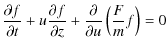
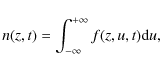
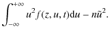
where z is the space coordinate, u is the velocity coordinate, F/m the non-conservative force per mass (acceleration), and f the phase space density (or probability density function). When f is known, the macroscopic quantities (density, velocity, energy) are moments of the distribution f. In particular, the zeroth order moment is the density n(z,t):
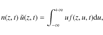
the first-order moment is the momentum (the product of the density by the macroscopic velocity
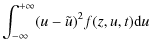
and the second-order moment is related to the pressure (a scalar in 1D):
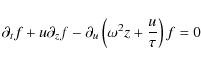
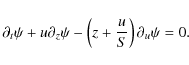
In the case of particles settling in a disk, there are two forces: gravity and gas drag. When the disk is geometrically thin, the vertical gravity can be written as
Under these conditions, Eq.
(1)
becomes
 |
(5) |
where z is now the vertical space variable and u the vertical velocity. To simplify the notations, we use the convention
 |
(6) |
The last term on the lefthand side (
At this point, it is convenient to adimension the time, introducing two new variables
![]() and
and
![]() .
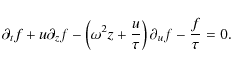
Using these new variables and omitting the primes for clarity, we get
.
Using these new variables and omitting the primes for clarity, we get
 |
(7) |
where
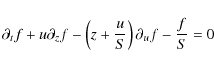
We now can artificially get rid of the exponential growth term by defining
 |
(8) |
and finally get
The behavior of this equation is rather easy to foresee. For infinite S, the remaining terms correspond to a rotation in phase space. This rotation is a direct consequence of energy conservation. In real space, particles oscillate around the midplane with zero velocity at the highest absolute altitude and maximum velocity when particles cross the midplane. The gas-drag term induces a collapse along the velocity axis. The net outcome of both the rotation and the collapse along the velocity axis (which corresponds in the real space to the dampening by gas drag of the inclination of the particle orbit) is a global collapse towards the center of the phase space (z=0, u=0), but not a spherical collapse.
3 Simple case
Although the general solution is given in the next section, it is useful to solve Eq.
(9) in the simplest case: infinitely large or massive particles (![]() ). In this case, the
equation admits a simple stationary solution with separated variables:
). In this case, the
equation admits a simple stationary solution with separated variables:

Using the definition of the moments, the pressure is straightforward:
where the density is
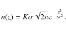
Equation (11) is similar to an equation of state for isothermal fluids, where
4 General solution
Equation (9) can be solved in the general case, using standard techniques (the method of characteristics for
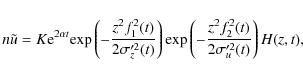
example). We will not develop this here as it is easier to check that the following solution is the general
solution of Eq. (9):
| (13) |
where
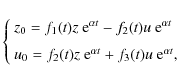 |
(14) |
where f1, f2 and f3 are time dependent functions given by
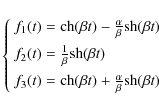 |
(15) |
and
![\begin{displaymath}\left\{
\begin{array}{ll}
\alpha=\frac{1}{2S}\\ [2mm]
\beta=\sqrt{(\alpha+1)(\alpha-1)}=\sqrt{\alpha^2-1}.
\end{array}\right.
\end{displaymath}](/articles/aa/full_html/2009/28/aa11865-09/img37.png) |
(16) |
Here,
5 Particular case for the initial conditions
Computing the moments of the phase space distribution cannot be done without the initial conditions.
Here, we choose an initial condition composed of Gaussians, with one Gaussian per dimension, which is relevant to most physically meaningful
cases:
where
5.1 The corresponding moments
Using definition (2), the density corresponding to the initial conditions (17) can be
written as
 |
(18) |
where the exponential dependencies can be included into the Gaussian widths:
![\begin{displaymath}\left\{
\begin{array}{ll}
\sigma_z'=\sigma_z {\rm e}^{-\alpha...
...2mm]
\sigma_u'=\sigma_u {\rm e}^{-\alpha t}
\end{array}\right.
\end{displaymath}](/articles/aa/full_html/2009/28/aa11865-09/img44.png) |
(19) |
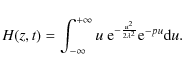
and L(z,t) is a function defined as
 |
(20) |
with
Let us define
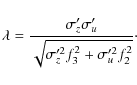
Then:
 |
(23) |
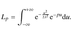
Here we keep the p-dependence explicitly as it will be useful in the following. We have L(z,t)=Lp if ptakes the value given by Eq. (21). This expression can be now written as
| Lp=F(p)+F(-p) | (24) |
where F(p) is the Laplace transform of a Gaussian:
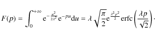 |
(25) |
Therefore, using the identity
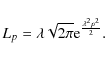
Using the definition (3) and a similar procedure, we get for the first-order moment:
 |
(27) |
where
 |
(28) |
Now Hp can be written as a function of Fp, using basic properties of the Laplace transform:
| (29) |
Hence,
 |
(30) |
Applying the same procedure to definition (4), we get the following expression for the particle fluid pressure:
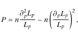 |
(31) |
and using Eq. (26), we finally get the simple expression for the pressure:
| (32) |
Here
It is interesting to note that the general pressure only depends on z through the density. The Euler equation for the particle fluid involves only gradients of the pressure so this gradient is in fact directly proportional to the density gradient. In other words, the particles seem to follow a barotropic equation of state. This behavior seems closely related to the assumption of constant stopping time (Garaud et al. 2004).
5.2 Scaling and asymptotics
5.2.1 Case  real (small particles)
When ![]() is real (and positive),
is real (and positive), ![]() is large, it is easy to check that
is large, it is easy to check that ![]() is a
decreasing function of time. Its initial value is
is a
decreasing function of time. Its initial value is
| (33) |
and the large time asymptotics are
 |
(34) |
Starting from a presumably very low value (the initial velocity dispersion of particles),
and
 |
(36) |
Even in the midplane, the pressure quickly drops with time, starting from a low value. In this case, as has long been known (see e.g. Garaud et al. 2004; Cuzzi et al. 1993; Dubrulle et al. 1995), it is safe to neglect the pressure of the particle fluid. Consequently, particles steadily sediment towards the disk midplane at a velocity close to the terminal velocity
5.2.2 Case
imaginary (large particles)
We define ![]() such that
such that
![]() .
In such a case,
.
In such a case, ![]() can be written as
can be written as
 |
(37) |
For small initial velocity dispersions, the location of the maxima of
 |
(38) |
and the amplitude of these maxima is
 |
(39) |
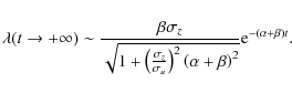
It is crucial to note here that the amplitude of the maxima of the time-dependent velocity dispersion
Since the midplane density is still given by Eq. (35), we get the amplitude of the midplane pressure
maxima:
 |
(40) |
These pressure maxima have a much lower decreasing rate than in the non-oscillating case, both because it involves only
The midplane pressure as a function of time for different values of the Stokes number S is displayed in
Fig. 1. The transition between the case with oscillation S > 1/2 and the overdamped case S <
1/2 appears very clearly. The pressure is computed for a ratio
![]() .
This ratio
defines the pressure at t=0 and the width of the maxima, but neither the amplitude of the maxima nor the decreasing rate.
.
This ratio
defines the pressure at t=0 and the width of the maxima, but neither the amplitude of the maxima nor the decreasing rate.
![\begin{figure}
\par\includegraphics[angle=270,width=8.5cm,clip]{11865fg1.ps}
\end{figure}](/articles/aa/full_html/2009/28/aa11865-09/img71.png) |
Figure 1:
Pressure of the particle fluid in the midplane as a function of the dimensionless time ( |
| Open with DEXTER | |
Figure 1 illustrates that, while the pressure of the solids fluid can be safely neglected for small
values of the Stokes number S, the situation is drastically different when the Stokes number reaches
S=1/2. When particles oscillate around the midplane, the fluid macroscopic velocity is different from
the terminal velocity ![]() as the macroscopic pressure force slows down the vertical contraction of the
particle fluid. In other words, the velocity of the particle fluid is not that of individual particles and the fluid
has a nonvanishing internal energy (contrary to the case for small particles).
as the macroscopic pressure force slows down the vertical contraction of the
particle fluid. In other words, the velocity of the particle fluid is not that of individual particles and the fluid
has a nonvanishing internal energy (contrary to the case for small particles).
6 Discussion and conclusions
We have shown that, in general, the pressure of the particle fluid cannot be neglected as soon as their Stokes number is more than 0.5. The particles seen as a fluid can have an internal energy, and the pressure force can partly balance gravity. In the extreme case where particles have an infinite inertia, the structure of the particle fluid is in fact hydrostatic. The existence of pressure is completely independent of the presence or absence of collisions between solid particles. Instead, the pressure is the result of a velocity dispersion. While velocity dispersion can be the result of collisions, it can also be created dynamically when external forces excite the velocity dispersion (gravity in the present case) or when the flow itself is converging locally. Even though our results concern only a very simple and specific problem, they have implications for a much broader variety of astrophysical and non-astrophysical flows.
The Stokes number can be defined in a more general way as the ratio of a dynamical timescale, creating velocity differences between the solids and the underlying fluid (gas or liquid), and the stopping time, the characteristic timescale for the particles to reach the fluid velocity. There are many processes able to create velocity differences between the gas and solids, gravity being only one of them. For example, when two rivers join, particles embedded in the rivers do not see the confluence like the water does and this can create a velocity difference between water and the particles, and a velocity dispersion in the particle flow at the confluence.
For particles embedded in a turbulent flow, it is common to define a scale-dependent Stokes number by
![]() ,
where
,
where ![]() is the turnover time of a turbulent eddy of size
is the turnover time of a turbulent eddy of size ![]() .
This Stokes number depends on the
size of the turbulent eddy and scales as
.
This Stokes number depends on the
size of the turbulent eddy and scales as
![]() for Kolmogorov-like turbulence
(see e.g. Cuzzi et al. 2001). The smallest reachable eddy is dependent on the strength of turbulence,
quantified by the Reynolds number of the flow
for Kolmogorov-like turbulence
(see e.g. Cuzzi et al. 2001). The smallest reachable eddy is dependent on the strength of turbulence,
quantified by the Reynolds number of the flow
![]() ,
where U and L are characteristic
velocities and length scale, respectively, and
,
where U and L are characteristic
velocities and length scale, respectively, and ![]() is the molecular kinematic viscosity of the fluid. For
Kolmogorov turbulence, the smallest turbulent scale
is the molecular kinematic viscosity of the fluid. For
Kolmogorov turbulence, the smallest turbulent scale
![]() of the flow scales as
of the flow scales as
![]() .
For flows with large enough Reynolds numbers (many astrophysical and geophysical flows reach
Reynolds numbers over 1010), the smallest turbulent scales have
.
For flows with large enough Reynolds numbers (many astrophysical and geophysical flows reach
Reynolds numbers over 1010), the smallest turbulent scales have ![]() smaller than 1, even
for small grains. This is a well-known behavior of particle-laden flows. Particles are centrifuged out of
the turbulent eddies whentheir scale Stokes number reaches unity (Squires & Eaton 1991). This creates a converging flow of
particles towards regions of low vorticity. Consequently, this induces a velocity dispersion inside the
particle flow and, for similar reasons to those described in this paper, the particle fluid develops a pressure. As a side note, when turbulence modelling is considered, turbulent pressure terms can arise from
fluctuating or subgrid velocity dispersions (Dobrovolskis et al. 1999). However, turbulent pressure terms are
a consequence of Reynolds averaging or spatial filtering and disappear when turbulence is directly simulated instead of
modelled.
smaller than 1, even
for small grains. This is a well-known behavior of particle-laden flows. Particles are centrifuged out of
the turbulent eddies whentheir scale Stokes number reaches unity (Squires & Eaton 1991). This creates a converging flow of
particles towards regions of low vorticity. Consequently, this induces a velocity dispersion inside the
particle flow and, for similar reasons to those described in this paper, the particle fluid develops a pressure. As a side note, when turbulence modelling is considered, turbulent pressure terms can arise from
fluctuating or subgrid velocity dispersions (Dobrovolskis et al. 1999). However, turbulent pressure terms are
a consequence of Reynolds averaging or spatial filtering and disappear when turbulence is directly simulated instead of
modelled.
This is hopefully a good illustration of the care one has to take whenever a fluid equation is applied to a collection of solid particles in an astrophysical flow. Whenever any dynamical timescale becomes smaller than the characteristic coupling timescale between the particles and the underlying fluid, the particles cannot be considered as a pressureless fluid, whatever the collision rate between particles.
Acknowledgements
Part of this work was done during the author's stay at Jeremiah Horrocks Institute for Astrophysics & Supercomputing, University of Central Lancashire, whose hospitality is gratefully acknowledged. I am grateful to J. Braine, S. Courty, B. Dubrulle, and J.-M. Huré for comments on the manuscript, and to the anonymous referee and T. Guillot for suggestions that helped me to significantly improve the presentation of the paper.
References
- Barrière-Fouchet, L., Gonzalez, J.-F., Murray, J. R., Humble, R. J., & Maddison, S. T. 2005, A&A, 443, 185 [NASA ADS] [CrossRef] [EDP Sciences]
- Carballido, A., Fromang, S., & Papaloizou, J. 2006, MNRAS, 373, 1633 [NASA ADS] [CrossRef]
- Cuzzi, J. N., Dobrovolskis, A. R., & Champney, J. M. 1993, Icarus, 106, 102 [NASA ADS] [CrossRef]
- Cuzzi, J. N., Hogan, R. C., Paque, J. M., & Dobrovolskis, A. R. 2001, ApJ, 546, 496 [NASA ADS] [CrossRef] (In the text)
- Dobrovolskis, A. R., Dacles-Mariani, J. S., & Cuzzi, J. N. 1999, J. Geophys. Res., 104, 30805 [NASA ADS] [CrossRef] (In the text)
- Dubrulle, B., Morfill, G., & Sterzik, M. 1995, Icarus, 114, 237 [NASA ADS] [CrossRef]
- Fromang, S., & Papaloizou, J. 2006, A&A, 452, 751 [NASA ADS] [CrossRef] [EDP Sciences]
- Garaud, P., Barrière-Fouchet, L., & Lin, D. N. C. 2004, ApJ, 603, 292 [NASA ADS] [CrossRef] (In the text)
- Guilloteau, S., & Dutrey, A. 1998, A&A, 339, 467 [NASA ADS]
- Hersant, F., Dubrulle, B., & Huré, J.-M. 2005, A&A, 429, 531 [NASA ADS] [CrossRef] [EDP Sciences]
- Inaba, S., Barge, P., Daniel, E., & Guillard, H. 2005, A&A, 431, 365 [NASA ADS] [CrossRef] [EDP Sciences]
- Johansen, A., Henning, T., & Klahr, H. 2006, ApJ, 643, 1219 [NASA ADS] [CrossRef]
- Lutsko, J. F. 1997, Phys. Rev. Lett., 78, 243 [NASA ADS] [CrossRef]
- Squires, K. D., & Eaton, J. K. 1991, Physics of Fluids, 3, 1169 [NASA ADS] [CrossRef] (In the text)
- Stepinski, T. F., & Valageas, P. 1996, A&A, 309, 301 [NASA ADS]
- Whipple, F. L. 1972, in From Plasma to Planet, ed. A. Elvius, 211 (In the text)
- Youdin, A. N., & Lithwick, Y. 2007, Icarus, 192, 588 [NASA ADS] [CrossRef]
All Figures
| |
Figure 1:
Pressure of the particle fluid in the midplane as a function of the dimensionless time ( |
| Open with DEXTER | |
| In the text | |
Copyright ESO 2009
Current usage metrics show cumulative count of Article Views (full-text article views including HTML views, PDF and ePub downloads, according to the available data) and Abstracts Views on Vision4Press platform.
Data correspond to usage on the plateform after 2015. The current usage metrics is available 48-96 hours after online publication and is updated daily on week days.
Initial download of the metrics may take a while.